Hardware study on the H.264/AVC video stream parser

Rochester Institute of Technology

RIT Scholar Works

Theses Thesis/Dissertation Collections

5-1-2008

Hardware study on the H.264/AVC video stream

parser

Michelle M. Brown

Follow this and additional works at:http://scholarworks.rit.edu/theses

This Thesis is brought to you for free and open access by the Thesis/Dissertation Collections at RIT Scholar Works. It has been accepted for inclusion in Theses by an authorized administrator of RIT Scholar Works. For more information, please [email protected].

Recommended Citation

Hardware Study on the H.264/AVC Video Stream Parser

by

Michelle M. Brown

A Thesis Submitted in Partial Fulfillment of the Requirements for the Degree of Master of Science in Computer Engineering

Supervised by

Dr. Kenneth Hsu,

Professor, RIT Department of Computer Engineering Department of Computer Engineering

Kate Gleason College of Engineering Rochester Institute of Technology

Rochester, New York May 2008

Approved By:

Dr. Kenneth Hsu

Professor, RIT Department of Computer Engineering Primary Adviser

Dr. Andreas Savakis

Professor, RIT Department of Computer Engineering

Dr. Dhireesha Kudithipudi

Dedication

I dedicate this thesis to my supportive family, who have always been there for me through

the good, the bad, and when I needed them the most. I would especially like to dedicate

this thesis to my mom, who provided me with the strength, courage, and determination to

always strive for my goals, and my dad, who encouraged me to pursue a college degree and

Acknowledgments

I would like to thank my advisors for proving their guidance, knowledge, and time during

Abstract

The video standard H.264/AVC is the latest standard jointly developed in 2003 by the

ITU-T Video Coding Experts Group (VCEG) and the ISO/IEC Moving Picture Experts Group

(MPEG). It is an improvement over previous standards, such as MPEG-1 and MPEG-2,

as it aims to be efficient for a wide range of applications and resolutions, including high

definition broadcast television and video for mobile devices. Due to the standardization of

the formatted bit stream and video decoder many more applications can take advantage of

the abstraction this standard provides by implementing a desired video encoder and simply

adhering to the bit stream constraints. The increase in application flexibility and variable

resolution support results in the need for more sophisticated decoder implementations and

hardware designs become a necessity.

It is desirable to consider architectures that focus on the first stage of the video

decod-ing process, where all data and parameter information are recovered, to understand how

influential the initial step is to the decoding process and how influential various targeting

platforms can be. The focus of this thesis is to study the differences between targeting

an original video stream parser architecture for a 65nm ASIC (Application Specific

In-tegrated Circuit), as well as an FPGA (Field Programmable Gate Array). Previous works

have concentrated on designing parts of the parser and using numerous platforms; however,

the comparison of a single architecture targeting different platforms could lead to further

insight into the video stream parser.

Overall, the ASIC implementations showed higher performance and lower area than the

FPGA, with a 60% increase in performance and 6x decrease in area. The results also show

Contents

Dedication. . . ii

Acknowledgments . . . iii

Abstract . . . iv

1 Introduction. . . 1

1.1 Background . . . 1

1.2 Thesis Objective . . . 2

1.3 Thesis Overview . . . 3

2 Video Compression . . . 4

2.1 Compression Techniques . . . 4

2.2 H.264/AVC Encoder and Decoder . . . 5

2.2.1 Encoding . . . 5

2.2.2 Decoding . . . 8

2.3 Existing Hardware Implementations . . . 10

3 H.264/AVC Video Stream Parser . . . 14

3.1 Reading NAL Units . . . 15

3.2 Parsing NAL Units . . . 17

3.2.1 Basic Coding . . . 18

3.2.2 Exponential-Golomb Coding . . . 18

4 Design and VHDL models . . . 21

4.1 Reading NAL units . . . 22

4.2 Parsing NAL units . . . 22

4.2.1 Basic Decoding . . . 23

4.2.2 Exponential-Golomb Decoding . . . 25

4.2.3 Context-Adaptive Variable Length Coding (CAVLC) . . . 27

5 Implementations and Testing . . . 42

5.1 ASIC Implementation . . . 43

5.1.1 Sub-Design Comparisons . . . 45

5.2 FPGA Implementation . . . 49

5.2.1 Sub-Design Comparisons . . . 50

5.3 Synthesis Simulations . . . 52

5.4 ASIC and FPGA Comparisons . . . 52

5.5 Comparisons with Existing Works . . . 54

6 Future Work . . . 56

7 Conclusion . . . 58

List of Figures

1.1 Structure of the H.264/AVC Video Stream Parser . . . 3

2.1 H.264 and MPEG-2 Comparison [3] . . . 6

2.2 Structure of an H.264/AVC encoder [8] . . . 6

2.3 Multi-Frame Motion Compensation [11] . . . 7

2.4 Integer Transform Matrix used in H.264/AVC [17] . . . 7

2.5 CAVLC Decoder [18] . . . 10

2.6 Low Power CAVLC Decoder Design [8] . . . 11

2.7 Low Cost High Performance CAVLC Decoder Design [6] . . . 12

2.8 Exp-Golomb Decoder [19] . . . 13

3.1 Video Stream Parser . . . 14

3.2 NAL Types [9] . . . 16

3.3 Example of CAVLC Decoding Reverse Zig Zag Scan . . . 20

4.1 Architecture of the Video Stream Parser . . . 22

4.2 NAL Unit Format . . . 23

4.3 NAL Unit Parser State Machine . . . 24

4.4 Hardware Design of the Exp-Golomb Decoder . . . 25

4.5 Hardware Design of the First One Detector used by the Exp-Golomb Decoder 26 4.6 Architecture of CAVLC Decoder . . . 27

4.7 Architecture for parse coeff token . . . 28

4.8 Neighboring Macroblocks of the Current Macroblock in Frame Mode . . . 28

4.10 State Machine Used By All Components Utilizing the Integer Division

Function . . . 30

4.11 Neighboring Macroblocks of the Current Macroblock in Field Mode . . . . 31

4.12 mbAddrN Specification with MbaffFrameFlag equal to One [17] . . . 33

4.13 Architecture of find luma neighbors . . . 34

4.14 State Machine for find luma neighbors . . . 35

4.15 State Machine Modeling the VLC look-up Tables . . . 36

4.16 Architecture of trailing1s level wrapper . . . 37

4.17 Architecture of totalZeros runBefore wrapper . . . 39

4.18 State Machine Modeling the totalZeros runBefore wrapper design . . . 40

4.19 Hardware Architecture for the Cofficients’ Array Indices . . . 41

5.1 16x16 Luma Block (left) and 8x8 Cb or Cr Block (right) . . . 42

5.2 The ASIC and FPGA Implementations’ Performance for Various Resolutions 44 5.3 Basic Decoding ASIC . . . 45

5.4 Exponential Golomb Decoding ASIC . . . 46

5.5 CAVLC Decoder ASIC . . . 46

5.6 Power, Area, and Performance Comparison of CAVLC Sub-Designs . . . . 47

5.7 parse coeff token ASIC . . . 48

5.8 trailing1s level wrapper ASIC . . . 48

5.9 totalZeros runBefore wrapper ASIC . . . 49

5.10 FPGA Resource Usage of Top Level Designs . . . 50

5.11 FPGA and ASIC Gate Count Comparison . . . 53

List of Tables

3.1 NAL Unit Format . . . 16

3.2 Entropy Decoder Algorithms . . . 17

3.3 Mapping of Exp-Golomb codeNums and Codewords . . . 18

3.4 CAVLC Decoder Syntax Elements [8] . . . 20

4.1 Neighboring Macroblock Address Calculations for Frame and Field Modes 31 4.2 mbAddrN Specification with MbaffFrameFlag equal to Zero [17] . . . 32

1. Introduction

1.1

Background

Video compression is the procedure through which the amount of data representing a video

sequence is significantly reduced to allow for a decrease in transmission time and an

in-crease in data storage by removing redundancies within the video. The need for video

compression arose with the development of technology and can be traced back to 1964

when AT&T introduced the first Picturephone at the World’s Fair in New York [10].

How-ever, a strong need came with the development of digital technology, such as

standard-definition television (SDTV), which was first introduced in 1996. Compared to analog

systems, SDTV offers more channels and produces better picture quality. SDTV displays

at a resolution of 704 X 480 pixels at 30 frames per second, which requires uncompressed

data to be transmitted at 121.7 Mbps. The MPEG-2 video compression standard is

com-monly used to handle the large amounts of video data the SDTV technology requires to be

sent by compressing the bit rate to 3 Mbps. One of the major advancements in television

af-ter SDTV is high-definition television (HDTV), which allows viewers to watch television

at even greater resolution. However, this implies more data to be transmitted during the

same amount of time. HDTV can be viewed at a resolution of 1920 X 1080 pixels, which

requires 746.5 Mbps of uncompressed data to be transmitted and about six times more data

to be sent than SDTV. The MPEG-2 standard is only able to compress the HDTV bit rate to

32 Mbps for HDTV [4]. As a result, a more advanced algorithm, such as the one specified

by the H.264/AVC standard, is desired to achieve an increase in transmission efficiency.

With the many techniques the H.264/AVC standard specifies, transmitting the same image

1.2

Thesis Objective

The objective of this thesis is to explore the design of the decoder’s first step, the video

stream parser, with a focus on providing an architecture to be targeted for two ASICs and an

FPGA. While existing implementations have shown to be valuable, the results of targeting

these designs for different platforms has yet to be studied. As a result of the thesis work

presented here, when an H.264/AVC video parser design is targeted for two ASIC process

technologies and an FPGA, insight is gained into the impact this decoder component has

across various process technologies and platforms. Since the video parser is composed of

numerous algorithms, the resulting architecture consists of original and leveraged designs,

where many designs were implemented as a Finite State Machine (FSM) and another used

different hardware components than seen in other published works.

The implementation satisfies the Basic H.264/AVC Profile, which can handle tasks such

as entropy decoding, macroblock adaptation of frame and field modes, and parsing

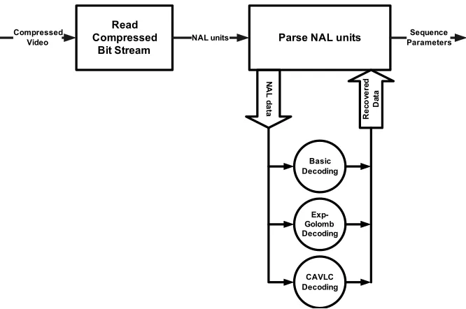
differ-ent slice types. The overall design is shown in Figure 1.1, where the first step is to read

the compressed video stream and parse the Network Abstraction Layer (NAL) units. The

NAL units, which are used to provide a layer of abstraction over the video data, are parsed

individually and various decoding algorithms are invoked, including Basic,

Exponential-Golomb (Exp-Exponential-Golomb), and Context-Adaptive Variable-Length Coding (CAVLC)

decod-ing, to recover all video data.

The VHDL hardware description language was used to describe an implementation of

the video stream parser. An existing behavioral model of the H.264/AVC decoder assisted

with the creation and validation of the synthesizable VHDL description. Implementing the

design allowed for the analysis of the parser with respect to the timing and hardware

com-plexities. The Xilinx ISE application was used to synthesize the FPGA model, while

Syn-opsys’ Design Compiler performed the synthesis of the lower power ASIC model.

Mod-elSim 6.1a SE was used to test the FPGA implementation, with the presumption that both

Read Compressed

Bit Stream NAL units Parse NAL units

Basic Decoding

Exp-Golomb Decoding

NA

L d

ata

R

ec

ov

er

ed

D

at

a

CAVLC Decoding

Sequence Parameters Compressed

Video

Figure 1.1: Structure of the H.264/AVC Video Stream Parser

1.3

Thesis Overview

An overview of video compression is given in Chapter 2, where various video compression

techniques, and an overview of the H.264/AVC standard are explored. The details of the

H.264/AVC video stream parser are presented in Chapter 3 and the design of the parser,

which includes how the NAL units are created and parsed, is presented in Chapter 4. The

three parsing methods, Basic, Exp-Golomb, and CAVLC decoding, are also explained in

this chapter. The testing strategies and statistics on the two implementations are given in

Chapter 5. Finally, the document is completed with a conclusion and future work

2. Video Compression

Video compression standards date back to the 1980s, when the first video codec

(en-coder/decoder) was standardized as the H.120 standard by the ITU-T. A decade later,

the MPEG group made vast improvements on video and audio compression and created

the MPEG-1 standard, which also defined the MP3 audio format and was used in Video

CD. Two years later, in 1991, MPEG expanded on their previous standard by creating the

MPEG-2, which specified the format of broadcast digital signals and stored digital video,

and is currently used in DVD standards and SDTV systems. The MPEG-2 was a vast

im-provement on the MPEG-1 because of its expansion of format specification and support

of interlaced video, which allows for the same video to be seen using half the bandwidth.

Later, in 1998, MPEG created the MPEG-4 standard, which aimed at the compression of

audio and video digital data and is currently used in many areas including web video, video

telephone, and broadcast television. There are several standards defined by the MPEG-4,

one of which is termed the ISO/IEC MPEG-4 Part 10 standard, or the ITU-T H.264

stan-dard, which is a digital video codec that is an improvement over previous standards by

flexibly providing high quality video data at various bit rates and has been around since

2003.

2.1

Compression Techniques

Different video compression techniques are available and can be classified into the

fol-lowing categories based on each technique’s goals: lossless, lossy, interframe, intraframe,

object, and transform based.

information and lossy compression discards some information to achieve a higher

com-pression ratio. Interframe comcom-pression takes advantage of temporal redundancies by using

the similarities between successive frames to reduce the amount of data required to

rep-resent the video sequence, while intraframe compresses each frame based solely on the

current one. The object-based technique compresses data based on the detection of

par-ticular objects between frames. Finally, transform based compression transforms the video

data from the spatial to frequency domain to exploit the human eye’s low sensitivity to high

frequency change. This is different from object-based because the entire image is divided

into blocks and the data is compressed independent of any objects within those blocks.

Parts of the 4 standard utilizes the object based compression, while the

MPEG-1, MPEG-2, and H.264/AVC standards use the transform based. The 2-D discrete cosine

transform (DCT), discrete wavelet transform (DWT), and the integer transform are some

methods used within transform based compression.

2.2

H.264/AVC Encoder and Decoder

The main goal of the H.264/AVC standard is to be efficient for a wide range of applications

and resolutions, while achieving lower bit rates than previous standards (see Figure 2.1).

The increase in application flexibility and compression ratio is enabled by the introduction

of many new features, such as context-adaptive variable length coding (CAVLC), weighted

prediction, multiple reference picture motion compensation, and an in-the-loop deblocking

filter.

2.2.1

Encoding

The H.264/AVC standard can be further explored by analyzing the encoding process

pre-sented in Fig. 2.2. The process encompasses four steps (motion estimation, transform,

quantization, and entropy coding), where each works on a 16x16 macroblock of video

Figure 2.1: H.264 and MPEG-2 Comparison [3]

- EstimationMotion Transform Quantization Entropy Coding

Inverse Quantization Inverse

Transform Uncompressed

Video CompressedVideo

Figure 2.2: Structure of an H.264/AVC encoder [8]

Motion Estimation

Motion estimation uses reference frames to detect change, or motion, between frames to

allow for only the residual data to be encoded. The video frames are classified into three

types: I, P, and B. An I-frame is encoded using intra-frame prediction, where macroblocks

within the frame are referenced, and can be used as a reference picture for subsequent

frames. A P-frame uses inter-prediction, where a previous frame is referenced to produce a

prediction signal for each block within the frame. The B-frame also uses inter-prediction,

but is able to reference two previous frames and take a weighted average of the two

predic-tion signal values [17]. The accuracy of the mopredic-tion representapredic-tion has been improved to

in-clude quarter-samples, compared to half-sample accuracy in previous standards. Also, the

allowance of motion vectors to breech picture boundaries has been added to the H.264/AVC

specification. The inclusion of using previously decoded pictures as reference for motion

Figure 2.3: Multi-Frame Motion Compensation [11]

Transform and Quantization

The H.264/AVC standard uses an integer transform algorithm on a 4x4 block, instead of

using a 4x4 DCT as in previous standards (see Fig. 2.4). The transformed coefficients are

then quantized, which is a lossy compression technique that divides the values and rounds

them to the nearest integer. This allows for greater compression efficiency because most of

the high frequency coefficients become zero [17].

Figure 2.4: Integer Transform Matrix used in H.264/AVC [17]

Entropy Coding

The output of the motion estimation, transformation, and quantization stages is sent through

a decoding feedback loop, where the difference between the incoming uncompressed video

and the processed data is recursively used in the encoding flow. The video data and settings

lengths by utilizing Exp-Golomb codes for all syntax elements, except for the quantized

transform coefficients, where CAVLC is used. The Exp-Golomb encoding scheme allows

for the use of only one look-up table, instead of having a table for each syntax element. The

CAVLC encoder is highly efficient and complicated; therefore, it is only used to encode the

quantized transform coefficients. There are multiple look-up tables used to encode the

various syntax elements associated with this scheme. More detailed information about the

Exp-Golomb and CAVLC schemes can be found in Chapter 3 - H.264/AVC Video Stream

Parser.

Video Coding Layer and Network Abstraction Layer

In the last stage, the Video Coding Layer (VCL) encoder provides a customizable

represen-tation of the video data and the Network Abstraction Layer (NAL) encoder adds headers

and organizes the data into NAL units. Having an abstraction layer, consisting of the VCL

and NAL layers, provides immense freedom for the application, while also adhering to the

standard.

2.2.2

Decoding

The process of decompression can be viewed as undoing the actions performed during

the compression process where similar techniques are used to recover the original video

data. Within a video sequence, each picture is divided into macroblocks, which represent

a fixed sized area of the picture. The fixed sizes of the macroblocks are 16x16 samples for

the luma component and 8x8 samples for the two chroma components. The H.264/AVC

standard separates the color representation of video into three components: Y,Cb,Cr, where

Y (or luma) refers to the brightness, and the Cb and Cr (or chroma) components refer to the

picture color with respect to blue and red. Since the human eye is more sensitive to change

in brightness than color, the luma component is represented with four times the amount

of samples than the chroma components. Equation 2.1 is used to calcuate the Y, Cb, Cr

(2.1)

A picture can also be represented as a frame, which embodies two interleaved fields.

The top field is made up of all even rows in the frame and the bottom field contains the odd

rows. Since moving objects often cause adjacent rows to be independent, compressing them

separately can provide greater coding efficiency. Conversely, non-moving objects should

be compressed in frame mode, since a dependency is likely to exist between adjacent rows.

The H.264/AVC standard supports adaptive field/frame encoding on a pair of macroblocks,

which allows for greater efficiency when a frame contains both moving and non-moving

areas [17].

The decoding process begins by parsing the incoming compressed stream and is

per-formed by the video stream parser. The decoder receives the data in NAL units, which are

packets that contain the encoded data, and are classified by the type of data they contain.

These units are parsed by the entropy decoder and depending on the type of NAL unit, a

specified entropy decoding algorithm is invoked. The three types of algorithms are based on

basic coding, Exponential-Golomb coding, and context-adaptive coding. After the stream

parser recovers all the parameter information and residual data, the inverse quantization

and transform stages reconstruct the residual data. Then, based on the type of prediction

used during encoding, the residual data is used to recreate the original frames. A side effect

of operating on blocks within each frame is visually noticeable block edges throughout the

frames. To smooth the edges of the blocking effect, H.264/AVC incorporates an in-loop

deblocking filter, which adapts its filter strength based on previous syntax elements and

2.3

Existing Hardware Implementations

High performance architectures of the H.264/AVC standard have been a focus of research

within many universities and in industry, but there has yet to be published studies focused

on a single architecture targeting different platforms. An industry example is one that

was a joint effort between Xilinx, Inc. and 4i2i Communication Ltd and is a main/high

profile decoder IP core for an FGPA. None of the implementation details have been

pro-vided, which prevents others from learning how they accomplished the design; however,

high level information has been given, such as the IP core targeting HD applications, the

fully pipelined design with multiple configuration options, and an external SRAM memory

needed to support the HD video [15].

There has also been some research performed on specific H.264/AVC decoder

compo-nents, namely the Context-Adaptive Variable-Length Coding (CAVLC) and Exp-Golomb

decoders. A proposed architecture, which focused on a generic VLSI architecture of the

CAVLC decoder, can be viewed in Figure 2.5.

R1 R0

32 bit Barrel Shifter 8 bit Accumulator Input

Level VLC

Decoder Controller

Coeff_token VLC Decoder

(VLD) Track_zeros

VLC Decoder Run_Before

VLC Decoder

# non-zero neighbor coeffs Coeff_token VLD done level VLD done

# zeros preceding non-zero coeffs

Total_coeff & T1 T1's sign & non-zero level # zeros before last level Length of consumed bits

Run

stack Level stack

The proposed CAVLC design is a pipelined architecture, which is suitable for

appli-cations requiring high throughput decoding due to the one cycle recovery time of a single

syntax element. The design consists of six components: the controller, input buffer,

co-eff token Variable Length Code (VLC) decoder, level VLC decoder, total zeros VLC

de-coder, and the run before VLC decoder. Since the end of each VLC is not known until the

previous VLC has been decoded, all actions occur sequentially. The input buffer aligns the

input stream so it is possible to decode the next code word, and the coeff token and level

VLC decoders determine which VLC table to use based on neighboring block information.

The total zeros VLC decoder determines the number of zeros preceding the last non-zero

level and the run before VLC decoder determines the number of zeros preceding the last

non-zero coefficient [18].

Another CAVLC decoder design is proposed for low power consumption and is targeted

as an ASIC using the 0.18um CMOS standard cell-based library (see Fig. 2.6).

Coeff_Token

TrailingOne

Level

Run_Before TotalZeros

Controller Output _Array Adder

Barrel Shifter R1

R2 Load

Codelength

maxNumCoeff reset vlctype

Code

Enable

Figure 2.6: Low Power CAVLC Decoder Design [8]

The design achieves its lower power consumption by employing various power saving

techniques, which include prefix predecoding and table partitioning within most of the

components. Another low power technique, which is used in the CAVLC design presented

Wishbone Interface Parameter Data Prediction Data R/W module Memory Coeff_Token Decoder TotalZero Decoder shifter T1 Decoder Level Decoder R E G IDS Controller acc Run_Before Decoder IQ

Figure 2.7: Low Cost High Performance CAVLC Decoder Design [6]

tables throughout the design. [8].

A low cost and high performance CAVLC decoder was proposed in [6], where various

techniques were used to achieve the real-time processing requirement of 1080 HD video

decoding (see Fig. 2.7).

To reach the high performance, this architecture contains a many more components

as the previous two designs, which include a Flush-unit, parameter interface, prediction

data R/W module, and Interleave Double Stacks (IDS). The Flush-unit flushes the previous

codeword into the bit stream and aligns the next one. The controller assists in

decreas-ing the computation time and lowerdecreas-ing the power consumption by implementdecreas-ing the Zero

Codeword Skip (ZCS), which does not decode zero codewords in 4x4 and 2x2 blocks that

only contain zeros. Also, placing an enable signal on each component allows for power to

be saved by disabling those which are not being used. Within the coeff token component,

hierarchical logic for look-up tables are used, which partitions the tables by frequency of

appearance and helps the design achieve its high performance goal. The IDS component

handles communication between the the CAVLC decoder and the inverse quantization [6].

A generic VLSI architecture for a Exp-Golomb decoder was proposed in [19] and a

modified version is presented in this thesis work. The proposed architecture can be viewed

R1 R0

32 bit Shifter 0 5 bit Accumulator

<<1 + 1 First 1 detector

Shifter1 32 – code_len

Postprocessing Module

input

carry

code_len M

Syntax element

Figure 2.8: Exp-Golomb Decoder [19]

The barrel shifter, ”Shifter0,” is used to align the input bit stream for the next decoding

cycle and the ”First 1 Detector” counts the number of leading zeros. The other barrel shifter,

”Shifter1,” is used to determine CodeNum + 1, which is used to determine the value of the

recovered syntax element. This architecture only requires 3210 gates with a critical path

3. H.264/AVC Video Stream Parser

A VHDL model of the video stream parsing process has been designed and successfully

implemented on two different platforms, a low cost FPGA and a low power ASIC. The

design was focused on the use of Finite State Machines and on the use of different

hard-ware components than seen in other published works. Also, low power techniques were

implemented to decrease the overall power consumption. Pipelining was not incorporated

into the design because of the inherent sequential bit reading of the incoming stream.

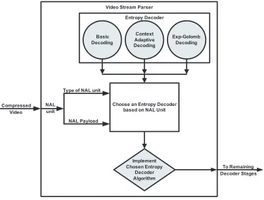
There are two main steps in achieving the functionality of the video stream parser:

reading NAL units and decoding the NAL units (see Fig. 3.1).

Video Stream Parser Entropy Decoder

Basic Decoding

Context Adaptive Decoding

Exp-Golomb Decoding

Implement Chosen Entropy

Decoder Algorithm Choose an Entropy Decoder

based on NAL Unit Compressed

Video

NAL unit

Type of NAL unit

NAL Payload

To Remaining Decoder Stages

The video parsing process consists of reading the compressed bit stream, creating the

NAL units, and parsing the NAL units to recover picture information. The parsing process

involves the use of three decoding components: Basic, Exp-Golomb, and CAVLC. The

Basic and Exp-Golomb decoders are used through out the video parsing scheme and return

a single syntax element, which could represent many slice header, sequence parameter, or

picture parameter values. The CAVLC decoder is a much more complex scheme and is

used to parse the residual, zig-zag ordered blocks of transform coefficients of each frame

to take advantage of the following quantized blocks’ characteristics:

1. Most non-zero coefficients tend to be toward the low frequency end of the zig-zag

or-dered list. As a result, VLC look-up tables are used to encode the level (magnitude).

2. Most of the values following the non-zero coefficients are (+/-) one; therefore, the

amount and sign of the trailing ones are encoded.

3. Each string of zero is encoded using run-level encoding since most of the quantized

blocks contain many zeros.

The top-level design consists of reading the data stream, iteratively parsing each unit,

and storing the recovered information. Most of the received units contain sampled values

of the video picture, while the units received at the start of the stream contain information

that could be applied to multiple units. Once all of them have been parsed and the video

parser completes, all the recovered data is sent to the next stage of the decoder.

3.1

Reading NAL Units

The creation of NAL units is the first step of the video stream parser. The compressed

video stream is read and based on the sequence of bits received, NAL units are created.

of data each one contains (see Fig. 3.2). The importance of the NAL is noticeable in its

ability to be efficiently customizable for various transport systems.

Figure 3.2: NAL Types [9]

Header Byte Payload

Forbidden zero bit Raw Bit Sequence Payload (RBSP) NAL reference ID

NAL unit type

Table 3.1: NAL Unit Format

The start of each unit is signified by a header byte, which holds various information,

as seen in Table 3.1. Following the header byte are payload bytes of the type specified in

the header. For systems that require the delivery of units in a byte-stream format, a start

code prefix is required to denote the beginning of each unit. Other systems, such as IP/RTP,

which is a protocol for delivering audio and video over the Internet, require the delivery of

them in packets; therefore, for these systems the use of the start code prefix is not necessary.

The payload can contain Video Coding Layer (VCL) or non-VCL data. The VCL NAL

contain parameter set information, which can be applied to multiple units and are values

that are not expected to change frequently. These parameter sets can be classified into

sequence parameter sets, which apply to a sequence of coded video pictures, or picture

parameter sets, which apply to separate coded video pictures.

A sequence of units that define a coded picture is called an access unit. There can also

be special NAL units that signify the beginning of an access unit, called an access unit

delimiter, and the end of an access unit, called an end of sequence or end of stream NAL

unit.

3.2

Parsing NAL Units

The task of the NAL parser is to analyze the incoming units to recover the video data,

header, and parameters. Based on the type of unit received, certain decoding algorithms are

invoked to recover the necessary syntax elements. The types of payloads that are encoded

can be categorized into Basic, Exp-Golomb, and context-adaptive syntax elements (see

Table 3.2).

Coding Algorithm Payload Type

Basic Byte

Basic Fixed-pattern n-bit string

Basic Signed n-bit integer

Basic Unsigned n-bit integer

Exp-Golomb Mapped Exp-Golomb-coded syntax element Exp-Golomb Truncated Exp-Golomb-coded syntax element Exp-Golomb Signed integer Exp-Golomb-coded syntax element Exp-Golomb Unsigned integer Exp-Golomb-coded syntax element Context-Adaptive Context-adaptive arithmetic entropy-coded syntax elements Context-Adaptive Context-adaptive variable-length entropy-coded syntax element

3.2.1

Basic Coding

The Basic decoding technique involves direct interpretation of each syntax element as the

type of element it was encoded as. For example, if an element was encoded as an unsigned

integer, then it is decoded as an unsigned integer. This technique handles the interpretation

of signed and unsigned integers, bytes, and fixed-pattern strings (see Table 3.2).

3.2.2

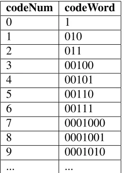
Exponential-Golomb Coding

The Exp-Golomb decoding algorithm is slightly more complex and uses a single

code-word look-up table (VLC table). Variable length coding uses smaller code code-word lengths

for frequently occurring data and larger codeword lengths for less frequently occurrences.

As a result, the average codeword length is reduced and higher compression is achieved.

Within the Exp-Golomb algorithm, the variable length codewords are defined as: [M

ze-ros][1][INFO], where M denotes the number of leading zeros and INFO denotes an M-bit

field of information. A codeNum value would have been mapped to its corresponding

codeword during the encoding stage.

codeNum codeWord

0 1

1 010

2 011

3 00100

4 00101

5 00110

6 00111

7 0001000

8 0001001

9 0001010

... ...

Table 3.3: Mapping of Exp-Golomb codeNums and Codewords

algorithms might be used (see Table 3.2). Each decoding algorithm determines the

code-Num value by using the equation codecode-Num = codeWord - 1. Then, based on the codecode-Num

calculated and decoding algorithm used, a corresponding element value is provided. These

element values are used to define certain video parameters and are passed to the remainder

of the decoder for further processing.

3.2.3

Context-Adaptive Variable Length Coding (CAVLC)

Context-Adaptive Variable Length Coding (CAVLC) decoding is a type of run length

de-coding, where the number of zeros to be transmitted is reduced. As a result of the

al-gorithm’s increased complexity and efficiency, it is only used when quantized transform

coefficients are transmitted. During video compression, many video coefficients become

zero after the quantization step occurs, which is termed a run of zeros. Instead of encoding

each zero into the video compression stream, run length compression is used, where the

run length of the zeros is encoded to increase the overall compression efficiency. CAVLC

decoding also uses the probability of occurring symbols to further increase the compression

ratio.

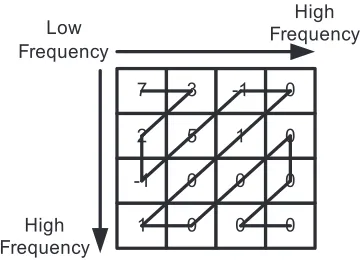
The CAVLC decoding algorithm receives the quantized coefficients within a

mac-roblock in zig-zag order, starting at the top left of the block (see Fig. 3.3). The low

fre-quency values are located in the top left and tend to have larger values than those at higher

frequencies. These values become less dense as the bottom right corner of the block is

approached.

The next step requires the decoding of five syntax elements from the received

coef-ficients: coeff token, sign of trailing ones (T1s), level, total zeros, and run before (see

Table 3.4).

The sign of the T1s and the level can be arithmetically decoded, while the other syntax

elements need to be decoded using look-up tables. There are two types of VLC tables

used: (1) for the number of non-zero coefficients and (2) for the level of the non-zero

7 3 -1 0

2 5 1 0

-1 0 0 0

1 0 0 0

Low Frequency

High Frequency

High Frequency

Scanned Coefficients: 7 3 2 -1 5 -1 0 1 0 1 0 0 0 0 0 0

Figure 3.3: Example of CAVLC Decoding Reverse Zig Zag Scan

Syntax Elements Description

coeff token the number of all non-zero coefficients (total coeff) and the number of trailing ones (T1s) are encoded by this syntax element

Sign of T1s the sign bit of each T1 is reverse zig-zag scan order is encoded by this syntax element

Level The value of each non-zero coefficient (except for T1s) is encoded by this syntax element

total zeros The total number of zero coefficients preceding the last non-zero coefficients in zig-zag order is encoded by this syntax element run before The number of successive zero coefficients following the non-zero

coefficients in reverse zig-zag order.

Table 3.4: CAVLC Decoder Syntax Elements [8]

choice is based on the values obtained from these blocks. Once a compressed bit stream

has been decoded, the pixel values of a 4x4 block can be recovered. When the final list

of coefficients have been compiled, they are passed onto the transform unit for further

4. Design and VHDL models

The video stream parser consists of three main functionalities: reading NAL units, parsing

NAL units, and a memory component (see Fig. 4.1). During the reading process, test

data is compiled into numerous NAL units and later parsed after all have been formed.

The recovery of all the picture parameter and data information occurs within the parsing

component, where the Basic, Golomb, and CAVLC decoders are utilized. The

Exp-Golomb and Basic decoding models are used by many other components because of their

ability to recover single syntax elements, which could represent the slice header, sequence,

or picture data, and are used as parameters by the remainder of the H.264/AVC decoder.

The majority of the video stream parser effort is located in recovering the slice data, which

represents the actual picture information, and where the CAVLC decoder is utilized. The

memory component is accessed to store and read the recovered data throughout the parsing

process. Also, the remaining stages of the H.264/AVC decoder will be able to read all of

the desired elements from this component.

The stream parser is modeled as a finite state machine to control the flow of data (see

Fig. 4.2). Reading of the NAL units begins when the stream parser is enabled and after

all units are read, the iterative parsing of each one commences. As each NAL is parsed

the recovered data is stored in a global memory component and the updated information is

available to all subsequent NAL units. After all parsing completes and the information is

saved, the design returns to its default state. By the end of this design, all appropriate data

Read in NAL units from test data

Parse NAL units NAL units

Recover Slice Header

Data NAL type = 1 or 5

Recover Sequence Parameters NAL type = 7

Recover Picture Parameters NAL type = 9

Recover Slice Data Main Memory Unit

(recovered data) Read/Write

Read MB Read MB Prediction Values

Recover Luma or Chroma MB from Residual Data

(CAVLC)

Exp Golomb

Decoding DecodingBasic Video Stream Parser

Figure 4.1: Architecture of the Video Stream Parser

4.1

Reading NAL units

Reading in the NAL units is accomplished by recursively reading a line from a hexadecimal

file until the end of the file is reached. Each line represents a byte of data, which is added

to the input buffer. The end of NAL units are detected by a delimiter, which is defined as

three consecutive bytes of zero followed by a fourth byte equal to one. When a delimiter

is detected, it is discarded and the NAL unit is created. At the end of this design, all NAL

units have been read in and are ready to be parsed.

4.2

Parsing NAL units

The goal of this design is to recover all necessary data from the NAL units. As each parser

algorithm is invoked, more information is found and could represent the slice header, data,

or parameter information. The design consists of much control logic for utilization of the

IDLE READ _NAL PARSE_NAL

CONTINUE PARSING PARSER

DONE

enable = 1 done = 1 parse

r_don_{e = 1}

coun t <= N

AL_co_unt

parser_do ne = 1

count > NAL_c

ount

-Save NAL output

-Save NAL output -Assign next NAL

input -assign NAL unit

-enable parser -increment NAL_count -enable reader

reset_n = 0

Figure 4.2: NAL Unit Format

is used to manage the flow of the design and is a vital part in the organization and control

of data. There are a total of eighty-six states within this design and a simplified version can

be viewed in Figure 4.3.

It can be noticed that the Basic and Exp-Golomb parsers are used by every state, which

signifies their importance in recovering single syntax elements throughout the video parsing

process. Even though the CAVLC parser is only used by one state, it constitutes the most

computational complexity and time consumption than the other two parsers. Its complexity

derives from the intensive algorithms it must endure to produce multiple coefficient values.

4.2.1

Basic Decoding

While the H.264/AVC standard specifies the Basic decoding scheme to decode signed and

unsigned integers, bytes, and strings, this design only has the capability to decode unsigned

integers and bytes. Since the CABAC decoding algorithm was not supported in this

im-plementation, the other two data types were not required to be decoded. As a result of the

algorithm’s simplicity, hardware was not required to be used; however, it was implemented

in this design to remain consistent with the rest of the video parser implementation. The

design of the basic decoding scheme takes in as input the current NAL payload and the size

of the desired syntax element, which could range from 1-bit to 8-bits. Since the range is

SEQUENCE

PARAMETERS PARAMETERSPICTURE SLICE

HEADER SLICE DATA

PARSE

NAL unit ty

pe = 1 or 5 NAL unit ty_{pe = 8} NAL unit type = 7

Basic

Exp-Golomb Basic

Exp-Golomb Basic _Golomb

Exp-READ MACROBLO

CKS

MB PREDICTION

SUB-MB PREDICTION

Basic

Exp-Golomb

Basic

Exp-Golomb CAVLC

Figure 4.3: NAL Unit Parser State Machine

element. Within the branches representing sizes 1 through 7 lies another case statement,

which provides all the bit configurations of the NAL payload for the particular syntax

el-ement size. Choosing this configuration allows for simple hardware representation by the

use of multiplexers to model the case statements. The 8-bit case is implemented using

the ”CONV INTEGER” function provided in the IEEE library since this function is more

efficient than using a 256-branched case statement for the 256 possibilities. The decoded

element is the integer equivalent to the bit configuration within the matched case statement

4.2.2

Exponential-Golomb Decoding

A structural approach is taken with the Exp-Golomb design and a modified version of [19]

is implemented, where a 32-bit accumulator and a 32-bit shift register are removed. The

re-moval of the unnecessary components provides an increase in performance due to the

Exp-Golomb decoding mechanism performing only one syntax element recovery at a time. As

a result, both an accumulator to track what bits of the input buffer have been consumed and

a register to shift the data in preparation for subsequent parsing are not needed. The

result-ing implementation has a decrease in complexity and power consumption. The hardware

design can be viewed in Figure 4.4 and consists of five components: first-one detector, two

bit shifters, an adder, and a post-processing module.

First 1 Detector R0

<< 1 M

32 - codeLength

2M

32-bit Shift right 16 bits 32 bits

Post-Processing Module codeNum + 1

32 – (2M + 1) = 31 – 2M

Syntax Element Input Data [0:31]

Figure 4.4: Hardware Design of the Exp-Golomb Decoder

An Exp-Golomb encoded codeword is formatted as [M zeros][1][M-bits of

informa-tion]. Given the maximum codeword length is 32-bits and the format of an Exp-Golomb

encoded codeword, it is a guarantee that the first 15 bits of data will contain a one.

MUX

Input (0:3) Input (4:7) Input (8:11) Input (12:15)

Encoder 1 Encoder 2

/4

+

/2 /4

M

Figure 4.5: Hardware Design of the First One Detector used by the Exp-Golomb Decoder

after the M-bits of zero. The 16-bit input is divided into four sections, each of which

determines if it contains a bit value of one. The four sections of bits are also sent to a

multiplexer where the selection is based on where the first detected one is located. The

output of the multiplexer is sent to an encoder, which produces a 2-bit value representing

the position of the one within the chosen section. The second encoder provides a 4-bit

value representing which of the four sections contained the first one. The output of both

encoders are added to produce the final output of this component, which is a 4-bit vector

specifying the bit location of the first detected one, denoted as M, within the given 16-bit

value.

The output of the first-one detector is sent to a shifter and adder to produce the code

length, which is defined as 2*M + 1. A modified version of this value (32 - code length) is

used by a 32-bit shifter to shift the input and produce (codeNum + 1), which is used by the

parser is controlled using a multiplexer that chooses the type of parsing to perform. If an

unsigned syntax element needs to be recovered, then the output is simply codeNum, and

when a mapped element is parsed a look-up is performed. When a signed or truncated

element is desired Eq. 4.1 or Eq. 4.2 are used, respectively.

syntaxelement= (−1)(codeN um+1)∗((codeN um+ 1)÷2) (4.1)

syntaxelement= (codeN um+ 1)%2 (4.2)

4.2.3

Context-Adaptive Variable Length Coding (CAVLC)

Coeff Token

Decoder TrailingOnes and Level VLC Decoder TotalZeros and RunBefore VLC Decoder Controller

Levels Memory

Accumulator 64-bit Shifter

64-bit Data Register Input Data

(32 bits)

Nonzero levels _{Nonzero levels}

# TotalCoeffs & # T1s # TotalCoeffs

# TotalCoeffs & # T1s

Coefficient array

T1 signs

Figure 4.6: Architecture of CAVLC Decoder

Out of three decoding algorithms implemented, the CAVLC is the most complex. This

design consists of thirteen hardware components, where the highest level is designed using

a large state machine to manage the data flow. There are three main components, which

1. parse the coeff token value to recover the amount of trailing ones and total

coeffi-cients (parse coeff token)

2. parse the number of trailing ones and level values for all non-zero coefficients

(trail-ing1s level wrapper)

3. parse the total amount of zeros and the location of each zero within the coefficient

array (totalZeros runBefore wrapper)

parse coeff token

Find Luma/Chroma Neighbor Information (find_luma_neighbors)

Determine which VLC table to use

Perform VLC table look-up

TotalCoeffs

T1s table ID

mbAddrA; blkIdxA

mbAddrB; blkIdxB block

index

Figure 4.7: Architecture for parse coeff token

This component is an original FSM-based (Finite State Machine) design to handle the

computational complexity and provide data flow management. The goal of this component

is to parse the coeff token codeword, which results in the production of two values: the

number of non-zero coefficients and trailing ones. These values are found via a VLC

look-up table, where the choice of table is dependent on the previously decoded macroblocks.

Figure 4.8 shows the naming conventions for neighboring macroblocks, where each ones

address and index in the macroblock array are found to help determine which look-up table

to use.

mbAddrD mbAddrB mbAddrC

mbAddrA CurrMbAddr

As a result of the computational complexity inherent in the parsing of the codeword,

FSM-based designs are used throughout the process to help control the massive amount

of data flow and use of many utility components. Figure 4.9 displays the components that

make up parse coeff token in a hierarchical organization. When the CAVLC component

is enabled, the 64-bit input buffer is filled from the incoming data stream to allow for

faster data access throughout this parsing procedure. The purpose of gathering the neighbor

information is to assist in determining which VLC table to use to find the total number of

coefficients and number of trailing ones.

parse_coeff_token

find_luma_neighbors

get_neighbor_location get_4x4_luma_scan

get_neighbor _mb_address getMacroblockIndex

mb_is_available divider

Figure 4.9: Hierarchical Organization of parse coeff token

• Division is used throughout the CAVLC decoding process. Even though division

by two can be executed as performing a bitwise shift right, there are many cases

where a divisor of two is not used. As a result, it is necessary to implement a integer

division design that can be used in the CAVLC process. The hardware components

and organization are derived from [13] and consists of four basic components: a

multiplexer, register, down-counter, and right-to-left shift register.

The usage of the division function is controlled by a state machine, shown in

Fig-ure 4.10, and is a part of all components that need to perform integer division.

Once the division is enabled, the numerator and denominator are assigned values,

these values are held at the input for two clock cycles to ensure proper signal

assign-ment within the block. When the division completes, the necessary output signals are

assigned to internal signals and during the final state they are latched into registers.

IDLE

Divider Enable

Divider Done

Compute Output

enable = 1 state_twice = 1

divider_

done = 1

Latch divider outputs into registers

Assign divider output to internal signals *Assign divider input values

*set “state_twice” signal reset_n = 0

Figure 4.10: State Machine Used By All Components Utilizing the Integer Division Func-tion

• mb is available determines if a macroblock is available and is accomplished by a

simple comparison with its address, the value of zero, and the current macroblock’s

address. The macroblock is available if it has a valid address, it is greater than zero,

and it is greater than the current one’s address, which would imply it has not been

analyzed.

• getMacroblockIndex determines a macroblock’s index in the macroblock array, which

is performed using a simple look-up into the array using the known address.

• get neighbor mb address finds all four neighboring macroblocks and returns their

addresses, if they exist. It supports macroblocks that are encoded in frame or field

mode, which could have been done independently on vertical pairs of luma

set denotes that the pair of macroblocks are coded in frame mode, otherwise they

are coded in field mode (see Figure 4.11). Table 4.1 shows how each neighboring

address is calculated depending on the value of MbaffFrameFlag, if they exist.

mbAddrD mbAddrB mbAddrC

mbAddrA CurrMbAddr or

CurrMbAddr

Figure 4.11: Neighboring Macroblocks of the Current Macroblock in Field Mode

Neighbor

Address Frame Mode Field Mode

mbAddrA CurrMbAddr - 1 2 * (CurrMbAddr/2 - 1)

mbAddrB CurrMbAddr - PicWidthInMbs 2 * (CurrMbAddr/2 - PicWidthInMbs) mbAddrC CurrMbAddr - PicWidthInMbs+1 2 * (CurrMbAddr/2 - PicWidthInMbs+1) mbAddrD CurrMbAddr - PicWidthInMbs-1 2 * (CurrMbAddr/2 - PicWidthInMbs-1)

Table 4.1: Neighboring Macroblock Address Calculations for Frame and Field Modes

• get 4x4 luma scan returns a block index when given a luma or chroma location

(xW,yW) by using Eq. 4.3. The division function previously discussed is

instanti-ated four times to handle the use of division used within this equation.

luma4x4BlkIdx = 4*(xW / 8) + 8*(yW / 8) +

1∗((xW%8)/4) + 2∗((yW%8)/4) (4.3)

• get neighbor location performs the functionality of finding a neighbor’s location

rel-ative to the upper left corner of the returned address. A neighboring macroblock

could contain luma or chroma type coefficients, where the size is expressed in terms

or chroma location, type of block, the MbaffFrameFlag signal, and the current

mac-roblock address, this component is able to produce a macmac-roblock address where the

given location resides as well as a new location expressed relative to the upper left

corner of the found address. This entity is implemented using six processes, where

the first one, depending on the value of MbaffFrameFlag, finds the macroblock

ad-dress, mbAddrN, or sets necessary flags for future use. Table 4.2 and Figure 4.12

show how the signal mbAddrN is assigned when given the luma or chroma location

(xN, yN). When the address is found, the location of the neighboring luma

loca-tion (xW, yW) is calculated relative to the upper left corner of mbAddrN using the

following equations:

xW = (xN +maxW H)÷maxW H (4.4)

yW = (yN +maxW H)÷maxW H (4.5)

xN yN mbAddrN

less than 0 less than 0 mbAddrD

less than 0 0 ... maxWH-1 mbAddrA

0 ... maxWH-1 less than 0 mbAddrB

0 ... maxWH-1 0 ... maxWH-1 CurMbAddr

less than maxWH-1 less than 0 mbAddrC

less than maxWH-1 0 ... maxWH-1 not available any value less than maxWH-1 not available

Table 4.2: mbAddrN Specification with MbaffFrameFlag equal to Zero [17]

• find luma neighbors finds the neighboring luma or chroma addresses and indices, if

they exist. Since the AVC Standard specifies the same algorithm for finding

neigh-bors of luma and chroma macroblocks, this component has the ability to find either

type of neighbor.

The data flow of the find luma neighbors component is shown in Figure 4.13. The

first step is to find the (x,y) location of the upper-left luma sample for the given 4x4

xN yN cu rr M bF ra m eF la g m bI sT op M bF la g m bA dd rX Ad di tio na l co nd iti on m bA dd rN yM yN yN (yN + maxWH) >> 1

2*yN yN yN yN yN >> 1 yN >> 1

yN yN yN yN yN yN na (yN + maxWH) >> 1

(yN + maxWH) >> 1 yN << 1 (yN << 1) - maxWH

(yN << 1) + 1 (yN << 1) + 1

-maxWH yN yN yN 2*yN 2*yN yN yN na na mbAddrD + 1

mbAddrA mbAddrA + 1 mbAddrD + 1 mbAddrD mbAddrD + 1

mbAdrrA mbAddrA mbAddrA + 1 mbAddrA + 1

mbAddrA

mbAddrB mbAddrB + 1

CurrmbAddr mbAddrC + 1

na mbAddrA mbAddrA + 1

mbAddrA mbAddrA + 1

mbAddrA mbAddrA + 1 mbAddrA + 1 mbAddrB + 1

CurrMbAddr - 1

mbAddrB + 1

mbAddrC + 1 mbAddrC mbAddrC + 1

na na

yN % 2 = = 0 yN % 2 ! = 0

yN % 2 = = 0 yN % 2 ! = 0

yN < ( maxWH / 2 ) yN >= ( maxWH / 2 ) yN < ( maxWH / 2 ) yN >= ( maxWH / 2 )

mbAddrD mbAddrA mbAddrA mbAddrB CurrMbAddr mbAddrC na mbAddrB CurrMbAddr mbAddrB mbAddrC mbAddrC na na 1 0 1 0 1 0 0 1 0 1 0 1 0 1 1 0 1 0 1 1 0 1 0 0 < 0 0 .. maxWH -1

0 .. maxWH - 1

< 0

< 0

0 .. maxWH - 1

> maxWH - 1

< 0

< 0

0 .. maxWH - 1

>

maxWH - 1

0 ..

maxWH - 1

> maxWH - 1

mbAddrD mbAddrD m bA dd rX Fr am eF la g 1 0 1 0 0 0 1 1 0 1 1 0 1 0 1 0 mbAddrA mbAddrA mbAddrA

Controller get_neighbor _location

(x,y) block location

mbAddrN (xN, yN) get_4x4_luma_scan

(xN,yN)

blkIdxN

block index

Current MB’s neighboring addresses and block

indexes (mbAddrA, blkIdxA;

mbAddrB, blkIdxB) MB Addresses

(from memory unit)

Figure 4.13: Architecture of find luma neighbors

x = InverseRasterScan( luma4x4BlkIdx / 4,8,8,16,0 )

+InverseRasterScan(luma4x4BlkIdxmod4,4,4,8,0) (4.6)

x = InverseRasterScan( luma4x4BlkIdx / 4,8,8,16,1 )

+InverseRasterScan(luma4x4BlkIdxmod4,4,4,8,1) (4.7)

Once a location is calculated, it is modified slightly so it would be possible to

cal-culate the location of the neighbors to the left and above the current macroblock.

The corresponding neighbor’s macroblock addresses and locations, relative to the

upper left corner of their containing macroblock, are then found by utilizing the

get neighbor location component previously discussed. Once the neighbor’s

ad-dresses (mbAddrA, mbAddrB) and corresponding locations ((xA,yA), (xB,yB)) are

found, the 4x4 luma or 4x4 chroma block index relative to the upper left corner of

the found macroblock is calculated using the get 4x4 luma scan component. The

This entity is designed as a ten-state state machine (see Fig. 4.14), where two

com-ponents previously described, get neighbor location and get 4x4 luma scan, are

en-abled and disen-abled as needed. The division function is also used to perform the

necessary division and modulation calculation to find the (x,y) location. If any of

the neighbors do not exist, their index is not attempted to be found. The found

in-dex(es) are saved to local signals and the state transitions to done state, where the

final outputs are latched.

Idle dividers_en dividers_done

compute_output

save_output

compute_vars

lumaScan_en find_neighbor_loc

find_blkIdx done_state

enable = ‘1’ state_twice = ‘1’

state_twice <= ‘1’

Both neighbors found Luma scans

completed reset_n = ‘0’

Calculate inputs to get_neighbor_location

component Latch division

outputs

Enable get_neighbor_location components and latch

their outputs Enable

get_4x4_luma_scan component(s) Latch final outputs

Latch appropriate get_4x4_luma_scan

outputs

Figure 4.14: State Machine for find luma neighbors

• coeff array models the coeff token VLC look-up tables and is implemented as a state

machine to manage the data flow (see Fig. 4.15). When this component is enabled,

the table to be used is determined based on an identification number passed in. The

parsing begins in the parse entry 0 state with a comparison between the first entry in

IDLE Find table Parse entry 0 End entry

reached

enable = 1

Latch outputs based on current table_entry value

reset_n = 0 _{Parse entry}

1

No LUT entry match LUT entry

match

Increment index value

*Increment table entry value *Reset index value

LUT(table_entry)(0 to index) !=

data(0 to index)

LUT(table_entry)(0 to index) ==

data(0 to index) LUT(table_entry)(index) == “X”

OR index = 16

OR table_entry = 62

Figure 4.15: State Machine Modeling the VLC look-up Tables

current table entry has been reached, if a full match has been found, if more

com-parisons are necessary, or if the end of the table has been reached. The comparison

between the current table entry and the input data is performed one bit at a time,

where an index value is used to determine where in the entry the comparison is

oc-curring. When the table entry and input data no longer match (NO LUT entry match),

the table entry value is incremented and the index value is reset to allow for the next

table entry to be examined for a match. Otherwise, if the table entry and input data

does match up to the current index value (LUT entry match), then the index is simply

incremented to continue the comparison between the two values. The end of a table

table entry size is reached. A successful full match is found when either of these

con-ditions are encountered during a comparison. Even though it is expected to always

find a match, the search would end if the table entry value exceeded 62 since there

are only 62 entries in the table.

trailing1s level wrapper

After the number of total coefficients (TotalCoeff) and amount of trailing ones

(Trailin-gOnes) are found using parse coeff token, the signs of the TrailingOnes and values of the

coefficients are calculated (see Fig. 4.16). This design is also original, where it consists of

three processes:

1. control the use of the level parser, latch the recovered level value, calculate the suffix

length based on that value

2. shift the data buffer after each level parser completion to allow for the next level

parser to retrieve data from the first data index

3. compile the final level values, which are based on the values of the TotalCoeff and

TrailingOnes signals, into an array

Recover T1 (+/-) signs

Recover non-zero coefficients (parse_level) 64-bit shifter

Amt consumed NAL payload data

Compile final array of coefficients (including T 1s) Amt consumed

Array of non-zero coefficients

The desired number of data bits is read from the input buffer to determine the sign of all

TrailingOne bits; this number is equivalent to TrailingOnes. The sign of the one is negative

when the data bit is zero and positive otherwise. Next, the values of the coefficients are

found by finding the level prefix and suffix values and respective lengths. With these values

the following equations are used to find the levels:

levelCode= (levelP ref ix∗(2suf f ixLength)) +levelSuf f ix (4.8)

For even-valued levelCode:

level= (levelCode+ 2)÷2 (4.9)

For odd-valued levelCode:

level = (−1? levelCode−1)÷2 (4.10)

Once the levels are compiled, they are serially written out to a memory element that

holds the recovered values and are used by the next design, totalZeros runBefore wrapper.

totalZeros runBefore wrapper

The final stage in performing the CAVLC decoding scheme involves two steps: (1)

recov-ering the total amount of zeros in the coefficient array and (2) determining the runs of zeros

between the already found level values. This original design encapsulates both algorithms

and controls their utilization with a state machine, whose diagram is shown in Figure 4.18.

The number of zeros are found by enabling parse total zeros and the runs of zeros are

found by enabling parse run before for each desired run value. Once all the necessary runs

are recovered, the final run value is assigned the remaining amount zeros. Based on the

runs of zeros found, the locations of the coefficients within an array are calculated with the

use of fifteen adders and multiplexers. The modeled architecture can be seen in Figure 4.19

Controller parse_total_zeros

TotalCoeff

total_zeros parse_run_before

run_before Shifter

NAL payload data

assign_coeffLevels

zero runs zeros_left Level Array

Coefficient Array

Figure 4.17: Architecture of totalZeros runBefore wrapper

dependent on the previous. Even though the range of TotalCoeff is fixed, the architecture

accounts for its dynamic value and is achieved by placing the multiplexers before the input

of one adder operand, where the previous coefficient location value could be used, if it

existed. The level values recovered by the trailing1s level wrapper component are then

placed where appropriate within the final coefficient array.

• parse total zeros and parse run before: Determining how many coefficients are

ze-ros and the location of the runs of zeze-ros consists of enabling a look-up table and

registering the results upon completion. A control signal is used to determine which

type of table to use: (1) finding the total amount of zeros for luma or chroma type

of neighbors, or (2) finding the runs of zeros. The total number of coefficients

(To-talCoeff) is used to choose a specific table to use. The actual table look-up process

is controlled using a state machine (see Fig. 4.11), where each table entry is read

and compared per bit to the data stream. Once a complete match is found, the

Idle

Enable

parse_total_zeros parse_total_zerosDone

Enable parse_run_before

parse_run_before Done Hold for data

stream Shifting enable = ‘1’

and totalCoeff > 0

zeros_done = ‘1’

totalCoeff > 1

run_done = ‘1’

Runs performed = (totalCoeff – 1) enable = ‘0’

reset_n = ‘0’

totalCoeff = 1

Runs performed < (totalCoeff – 1)

Assign Last Run Value Assign

coefficient array values