Representation decomposition for knowledge extraction and sharing using restricted Boltzmann machines

(1)

City, University of London Institutional Repository

Citation

:

Tran, Son (2016). Representation decomposition for knowledge extraction and sharing using restricted Boltzmann machines. (Unpublished Doctoral thesis, City University London)

This is the accepted version of the paper.

This version of the publication may differ from the final published

version.

Permanent repository link:

http://openaccess.city.ac.uk/14423/

Link to published version

:

Copyright and reuse:

City Research Online aims to make research

outputs of City, University of London available to a wider audience.

Copyright and Moral Rights remain with the author(s) and/or copyright

holders. URLs from City Research Online may be freely distributed and

linked to.

(2)

KNOWLEDGE EXTRACTION AND SHARING USING

RESTRICTED BOLTZMANN MACHINES

by

Son Tran

A thesis submitted in fulfilment of the requirements for the degree of Doctor of Philosophy, Department of Computer Science,

City University London.

(3)

(4)

Abstract

Restricted Boltzmann machines (RBMs), with many variations and extensions, are an efficient neural network model that has been applied very successfully recently as a building block for deep networks in diverse areas ranging from language generation to video analysis and speech recognition. Despite their success and the creation of increasingly complex network models and learning algorithms based on RBMs, the question of how knowledge is represented, and could be shared by such networks, has received comparatively little attention. Neural networks are noto-rious for being difficult to interpret. The area of knowledge extraction addresses this problem by translating network models into symbolic knowledge. Knowledge extraction has been normally applied to feed-forward neural networks trained in supervised fashion using the back-propagation learning algorithm. More recently, research has shown that the use of unsupervised models may improve the perfor-mance of network models at learning structures from complex data. In this thesis, we study and evaluate the decomposition of the knowledge encoded by training stacks of RBMs into symbolic knowledge that can offer: (i) a compact representation for recognition tasks; (ii) an intermediate language between hierarchical symbolic knowledge and complex deep networks; (iii) an adaptive transfer learning method for knowledge reuse. These capabilities are the fundamentals of a Learning, Extrac-tion and Sharing (LES) system, which we have developed. In this systemlearning can automate the process of encoding knowledge from data into an RBM, extrac-tionthen translates the knowledge into symbolic form, andsharingallows parts of the knowledge-base to be reused to improve learning in other domains. To this end, in this thesis we introduceconfidence rules, which are used to allow the com-bination of symbolic knowledge and quantitative reasoning. Inspired by Penalty Logic - introduced for Hopfield networks confidence rules establish a relationship

(5)

between logical rules and RBMs. However, instead of representing propositional well-formed formulas, confidence rules are designed to account for the reasoning of a stack of RBMs, to support modular learning and hierarchical inference. This approach shares common objectives with the work on neural-symbolic cognitive agents. We show in both theory and through empirical evaluations that a hierar-chical logic program in the form of a set of confidence rules can be constructed by decomposing representations in an RBM or a deep belief network (DBN). This decomposition is at the core of a new knowledge extraction algorithm which is com-putationally efficient. The extraction algorithm seeks to benefit from the symbolic knowledge representation that it produces in order to improve network initialisa-tion in the case of transfer learning. To this end, confidence rules offer a language for encoding symbolic knowledge into a deep network, resulting, as shown em-pirically in this thesis, in an improvement in modular learning and reasoning. As far as we know this is the first attempt to extract, encode, and transfer symbolic knowledge among DBNs. In a confidence rule, a real value, namedconfidence value, is associated with a logical implication rule. We show that the logical rules with the highest confidence values can perform similarly to the original networks. We also show that by transferring and encoding representations learned from a domain onto another related or analogous domain, one may improve the performance of representations learned in this other domain. To this end, we introduce a novel algorithm for transfer learning called “Adaptive Profile Transferred Likelihood”, which adapts transferred representations to target domain data. This algorithm is shown to be more effective than the simple combination of transferred representa-tions with the representarepresenta-tions learned in the target domain. It is also less sensitive to noise and therefore more robust to deal with the problem of negative transfer.

(6)

Acknowledgements

First and foremost I would like to thank my supervisor Artur d’Avila Garcez for supporting me through all the hard work to complete my PhD thesis. The encour-agement and inspiration he has brought to me since the first day I came to City University London (the City) have great influence to my work. Artur is not only an experienced supervisor but also my research companion who shares with me the fun and the beauty of AI. He can spend hours to listen to my explanations, most of which I barely understand if I do this to myself.

I am fortunate to have an opportunity to work with many excellent researchers at the City, especially Tillman Weyde, Daniel Wolffand Srikanth Cherla in applying representation learning and deep learning to music informatics. I also enjoyed collaborating with Emmanouil Benetos (QMUL) in the work of action recognition, Thanh Vu (OU) in search personalisation and Hazrat Ali (USTB) in speaker recogni-tion. During my time at City, I have received huge support from the administrative and technical staff, especially Mark Firman and Chris Marshall.

I gratefully acknowledge the funding source that made my Ph.D work possible. For this, I would like to thank Jason Dykes for supporting my application, and after that, my work as the second supervisor. My research was funded by the studentship from City University London. During my PhD years I have received a number of other funds from City to attend conferences and workshops. I also want to thank Chris Child for having me in the pump-priming project. This funding allows me to establish the ideas of future work during the writing up.

For the completion of this thesis I would like to extend the sincerest appreciation to Daniel Silver, Emmanouil Benetos, Srikanth Cherla, Manoel Franca, Andrew

(7)

Lambert, Muhammad Asad, Nathan Olliverre, Rilwan Basaru and Hazrat Ali, who have spent their precious time to read and give me valuable comments. I want to send my deep gratitude to Kostas Stathis and Gregory Slabaugh for the fair examination of my thesis and for their constructive suggestions.

(8)

List of Figures

1.1 LES triangle: learning from data, knowledge extraction, and sharing

for transfer learning. . . 2

2.1 A Hopfield network (s={_a,_b}_{). . . 20}

2.2 A Boltzmann machine. . . 21

2.3 A restricted Boltzmann machine. . . 23

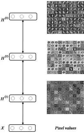
2.4 A stack of RBMs trained on handwritten digits with visualisations of the units in the hidden layers obtained by activating each hidden unit at a time and performing downward inference to the visible layer thus generating pixels for the images. The hierarchy is expected to model levels of abstraction by transforming the feature vectors, in this case from edges to shapes and finally digits. . . 32

2.5 Visualisation of 24 filter bases from RBMs trained on motion-difference of (a) Weizmann and (b) KTH datasets. . . 32

2.6 Visualisation of the filter bases of a Gaussian RBM trained on spec-trograms of different types of music. . . 33

3.1 A Boltzmann machine for the XOR formula. . . 37

3.2 RBM for XOR formula: (x⊕_y₎↔_z_{. . . 42}

3.3 RBM for CIFFs. . . 44

(15)

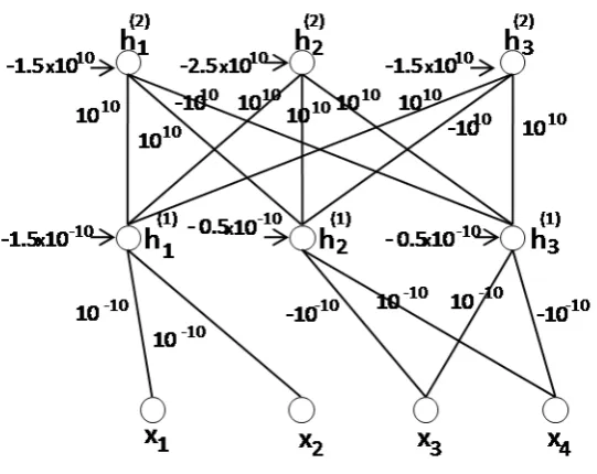
3.4 A DBN forx₁∧_x₂∧₍_x₃⊕_x₄_{). . . 45}

3.5 Networks for CIFF (N1) and confidence rule (N2). . . 47

3.6 DBN corresponding tox₁∧_x₂∧₍_x₃⊕_x₄_{). . . 48}

4.1 Converting a sub-network in original RBM to new sub-network in easy-to-interpret RBM. . . 53

4.2 Error rate progression in comparison with memory capacity gains for RBMs and the extracted rules pruned by 0, 20, 40, 60 and 80%. . . 65

4.3 Classification performances of RBMs and the extracted rules on DNA promoter dataset. . . 68

4.4 Classification performances of DBNs compared with extracted rules on the DNA promoter dataset. . . 68

4.5 Comparison between the test-set accuracies of DBNs (model accu-racy) and extracted rules. . . 73

4.6 Comparison between the test-set accuracies of DBNs (model accu-racy) and extracted rules using rule-based early stopping. . . 73

4.7 DBN obtained from hierarchical rule setKfrom Example 4.4.1. . . 75

4.8 A deep neural-symbolic integration with 5 rules have been encoded. 79

4.9 Test set classification performance of 2-layer standard DBN (red and black lines, with and without model selection), and 2-layer DBN encoded with prior knowledge from the DNA promoter background theory using training sets with 10, 30, 50 and 70 samples, and 20 test samples. . . 80

(16)

5.1 Sub-networks for partial model in Eq. 5.4 and complete model in Eq. 5.3, respectively. As we can see, the weights in the sub-network representing a partial model have the discrete values{c,0,−_c}_{, while}

the weights of the sub-network representing a complete model have real values, similar as the weights of RBMs. . . 89

5.2 Feature detectors learned from RBM on MNIST dataset. . . 89

5.3 Feature detectors from sparse RBM on MNIST dataset. . . 90

5.5 Classification accuracy of a pruned RBM, starting with 500 hidden units, on 10,000 MNIST test samples. The red and blue lines repre-sent the accuracy following pruning of low-scoring and high-scoring feature detectors respectively. . . 91

5.6 Mutual Information measurement on ranked feature detectors. . . . 92

5.7 General representation transfer model for unsupervised learning. . . 95

5.8 Self-taught learning using RBMs where only a subset of features have been transferred. . . 97

5.9 Performance of learning with guidance for different numbers of transferred complete-models and additional hidden units. The colour-bars map accuracy to the colour of the cells as shown so that the hotter the colour, the higher the accuracy. . . 99

6.1 aTPL example of transferring representations from Plus image to Minus image. . . 102

6.2 Number of complete-models/feature detectors in the adaptive part and in supplementary part of aTPL in four scenarios. . . 111

(17)

6.4 The corrupted representations and their transform after applying Algorithm 8 on 2000 MNIST test samples. For each sub-figure, the left picture shows the corrupted representation and the right picture show the representation after the learning. . . 113

7.1 Proposed deep relational model. . . 122

E.1 Filter bases from RBM trained on Frey face images. The RBM has 500 units in hidden layer, the learning rate η = 0.01, sparsity gain λ =0.1 (p =0.00001). The bases are organised in descending order of their scores from top to bottom and from left to right. . . 151

(18)

List of Tables

1.1 Probability table of the “plus” shape graphical model. . . 4

3.1 XOR formula and Penalty logic ranking. . . 37

3.2 Truth table of XOR formula: (x⊕_y₎↔_z_{. . . 39}

3.3 Energy function and truth table of XOR formula. . . 40

3.4 Minimised energy function of RBM representing truth-table of XOR formula. . . 42

3.5 Truth-table of conjunction x∧ _y _{and energy of the networks} con-structed from CIFF h ↔ _x∧_y _{and confidence rule 5 :} _h ↔ _x∧_y respectively. . . 47

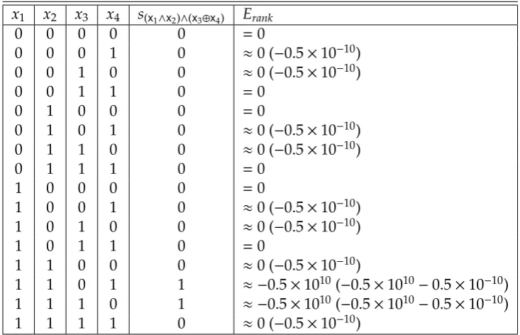
3.6 Truth table of (x₁∧_x₂₎∧₍_x₃⊕_x₄_{) and the minimised energy of all} possible input state of DBN constructed from confidence rules. . . 49

4.1 Truth-table of XOR function. . . 57

4.2 Rules extracted from RBM trained on XOR function. . . 58

4.3 Inference of z from the confidence rules extracted from an RBM trained on the XOR truth-table. . . 58

4.4 Car evaluation data description. In the second (“label”) column “Yes/No” indicates whether the variable is the label or not. . . 58

(19)

4.5 The expected memory saving ratios for an RBM with 784 visible units and 500 hidden units using standard floating point data types in a 32-bit computer;pruningrefers to the percentage of the removed hidden nodes which correspond to the rules with low confidence values. . . 64

4.6 Average test set performance of RBMs in comparison with their low-cost representation on four different datasets. The table shows the prediction accuracy of the SVMs trained on the features extracted from the model (RBMs) and the features extracted from the rules (Low-cost). . . 64

4.7 Hierarchy of rules from background theory in the DNA dataset; the first four rules appear in levelL−_{1 of the hierarchy, then level}_L−_2,

and so on. Each level will be mapped onto a layer of a DBN. . . 78

5.1 RBM trained on XOR function and one of its sub-networks with score value and logical interpretation. . . 87

5.2 Sub-networks and scores from RBM with 10 hidden units trained on XOR truth-table. . . 88

(20)

6.1 Transfer learning experimental results: each column indicates a transfer experiment, e.g. MNIST30k:ICDARd uses the MNIST

hand-written digits (with 30,000 samples) as the source domain and the natural digit images ICDAR as the target domain. The percentages show the average predictive accuracy on the target domain with a 95% confidence interval. Results for SVMs are provided as a base-line. For the “SVM” and “RBM” lines, there is no transfer. The bold number indicates a statistically significant improvement. If the improvement is not apparent, then it indicate more compactness in terms of the model’s capacity. . . 110

6.2 Negative transfer with corrupted representation from the source do-main, trained on 20,000 MNIST samples. The representations are flattened, flipped, and combined of both effects. The target domain is the MADBASE data set consisting of Hindi handwritten digits from 10 writers. The bold numbers indicate that the improvement is statistically significant. . . 113

A.1 Comparison of original features and those with PCA and RBM pre-processing in terms of similarity prediction accuracy. Test and train-ing set results are listed as percentages of correctly predicted similar-ity constraints for the configurations with the best training success. The SVM original values are taken from [141]. . . 135

A.2 Performance on Weizmann dataset. The results of [146, 99, 139, 84] are copied from the original papers . . . 137

A.3 Performance on KTH dataset. Results of [99, 139, 123, 142, 24, 74] are copied from the original papers . . . 137

A.4 Test set accuracy for speaker classification . . . 138

(21)

(22)

(23)

Notations

Matrices, vectors are denoted using bold capital (X), boldface (x) letters respectively. A constant is denoted as normal capital letter (N). Italic letters (E, f,g) denote a function. Concatenation of matrices/vectors are denoted as [X,Y] for column order and [X;Y] for row order. A subscript is used to denote an element in a matrix and vector, for example xi j and xi. A vector xj denotes the column j of matrix

X. A proposition is denoted as x while a numerical variable is denoted asx. A propositionxhas two possible valuestrueand f alsewhich is equivalent to a binary variablexwhich has values 1 and 0 respectively.

The transpose of a matrix or a vector is denoted byX>andx>respectively. In a group of numbers such as 1, 2, ..., ,N,\_i_{denotes a subset of the group that contains}

all numbers excepti. For different types of product, matrix/vector multiplication is denoted asXY, while×_{denotes the scalar multiplication and}◦_denotes

element-wise product. The notation=is used for assigning a value to a variable, while∼_is

used for sampling from a distribution.

Probability distribution of a variablexis denoted asp(x). With a binary variable x,P(x) denotesp(x=1) andP(x|_{y) denotes}_p(x=₁|_y).

Logical connectives such as NOT, AND, OR, XOR, IF-THEN, and IF-AND-ONLY-IFare denoted using standard notation¬_,∧_,∨_,⊕_,←_,↔_{respectively. We use}

V

ixito denotex1∧x2....andWito denotex1∨x2...

In a hierarchical structure, superscripts are used to denote the levels. For example, in a multilayer network a state of visible layer is denoted asxand state of a hidden layerl(l>0) is denoted ash(l). If a network has only two layers,h(1)can be replaced byhfor ease of presentation. The set of all parameters of a network is denoted asθ.

(24)

Abbreviations

aTPL Adaptive Transferred Profile Likelihood BM Boltzmann Machine

CNF Conjunctive Normal Form CD Contrastive Divergence CIFF Conjunctive If-And-Only-If DBN Deep Belief Network DBM Deep Boltzmann Machine DNF Disjunctive Normal Form GSTL Guided Self-taught Learning KL Kullback-Leibler

NN Neural Network

NSCA Neural-Symbolic Cognitive Agent MI Mutual Information

PCA Principal Component Analysis PLOFF Penalty Logic Well-formed Formula RBM Restricted Boltzmann Machine SAE Stacked Auto-Encoder

SC Sparse Coding

SDNF Strict Disjunctive Normal Form STL Self-taught Learning

SVM Support Vector Machine WFF Well-formed Formula

(25)

(26)

Introduction

Unsupervised models such as restricted Boltzmann machines (RBMs) and deep be-lief networks (DBNs) can learn useful patterns for recognition tasks in wide range of domains. In addition, these patterns have been shown to capture domain rep-resentations at different levels. For example, visualisation of the patterns learned from handwritten image data indicates that low level patterns represent curves and edges while the higher level patterns represent more concrete shapes. This interesting characteristic of unsupervised learning intrigues a question of whether symbolic knowledge can also be represented by these patterns. This chapter takes this question as a starting point to propose a research on decomposition of represen-tations in RBMs/DBNs to build a Learning, Extraction and Sharing (LES) system.

1.1 Motivation

RBMs, with many variations and extensions, are an efficient neural network model that has been applied very successfully recently as a building block for deep net-works in diverse areas ranging from language generation to video analysis and speech recognition. Despite their success and the creation of increasingly complex network models and learning algorithms based on RBMs, the question of how knowledge is represented, and could be shared by such networks, has received comparatively little attention. Breiman argues that one can enjoy the effectiveness of complex systems while knowledge should be produced separately for

(27)

tion purposes [19]. This motivates the development of a learning, extraction and sharing system as illustrated in Figure 1 [19].

Figure 1.1: LES triangle: learning from data, knowledge extraction, and sharing for transfer learning.

The exponential growth of digital content has required the development of robust, flexible, modular and expressive systems in order to handle the challenges of Big Data. In order to achieve this while being able to provide interpretability, the ideal system should embody the capabilities oflearning,extractionandsharing of knowledge given rich, complex data. More specifically, learningcan automate the process of encoding knowledge hidden in a large data set, knowledgeextraction from a trained model can further translate the knowledge into more readable forms such as symbolic or visual languages, and help highlight the relevant knowledge. It also promotes explicit reasoning, as will be exemplified in what follows. Finally, such knowledge can be used forsharing, i.e. to improve the learning in another related task. To realise all these capabilities one has to address the following challenging research questions:

• _{How should knowledge be represented?} • _{how can it be achieved from data?}

• _{How to transfer it from one domain to another?}

1.1.1 Knowledge Representation and Learning

(28)

refers to symbolic knowledge to which reasoning can be applied systematically. In classical logic, propositional logic is one of the most basic and popular symbolic languages, built upon propositions and the logical connectives “and”, “or”, “nega-tion”, “implica“nega-tion”, and “bi-conditional”[118].Propositionsare particular kinds of sentences which only have either atrueor f alsevalue. Connectivesare the symbols which are used to construct complex sentences from simpler ones. For example,

a 3×_{3 black and white image} _{may represent a “plus” sign. If the pixels are}

numbered in the order from left to right, top to bottom, the symbolxi can be used

to represent the proposition ”pixel i is white”. The symbol¬_x_i _{then represents the}

proposition “pixel i is not white”. Together with the proposition that there are only white or black pixels in this case, the above propositions can be reasoned with to conclude that “pixel i is black”. Let the symbol plus denote the proposition “the picture is a plus sign”. In a closed world with 9 variables denoting the values of the

9 pixels, knowledge about the plus sign can be represented by the following logical rule, indicating thatplusis true ifx₁is false,x₂is true, etc:

plus← ¬_x₁∧_x₂∧ ¬_x₃∧_x₄∧_x₅∧_x₆∧ ¬_x₇∧_x₈∧ ¬_x₉

In other words, we have used a set of symbols to represent visual information. By encoding knowledge into a symbolic form, one may be able to reason about such knowledge in a precise way which follows the rules of logical inference [117].

In order to support more flexible reasoning, however, especially under uncer-tainty, knowledge can be represented by probabilistic models. For example, a Bayesian network [103] encodes knowledge into a dependency graph and proba-bility tables. Let us consider the same “plus sign” example above, where we can treat a pixelias a binary variablexi ∈ {0,1}, withxi = 1 indicating that the pixel

is white and xi = 0 indicating that it is black; plus ∈ {0,1} indicates whether the

picture is a plus sign (plus=1) or not (plus=0). A Bayesian network represents the knowledge in this domain as a graphical model with distribution table as shown in Table 1.1. The table assigns a high probability of 0.8 to the “plus” shape, a probability of 0.022 to all the shapes that have only one pixel different from the “plus” shape, and probability 0 to all the other shapes.

(29)

x1 x2 x3 x4 x5 x6 x7 x8 x9 p(plus=1|x1,x2,x3,x4,x5,x6,x7,x8,x9)

0 0 0 0 0 0 0 0 0 0

...

0 1 0 1 1 1 0 0 0 0.022

0 1 0 1 1 1 0 0 1 0

0 1 0 1 1 1 0 1 0 0.8

0 1 0 1 1 1 0 1 1 0.022

...

1 1 1 1 1 1 1 1 1 0

Table 1.1: Probability table of the “plus” shape graphical model.

representation is more complex. For example, the probability that the picture is a plus sign given the values of a large number of pixels is

P(plus|_x₎=_pdf₍_x, θ)

wherexis a vector denoting the set of all variables andpdfis a probability distri-bution function.

Learning algorithms applied to neural networks [49] and Bayesian networks [103] have been shown capable of representing rich knowledge, being particularly useful in the case of noisy data. Neural networks, however, in spite of their success, are difficult to interpret. The area of knowledge extraction [6, 136, 31] seeks to address this problem mainly by translating the networks into symbolic knowledge. Knowledge extraction has been normally applied to feed-forward neural networks trained in supervised fashion using the back-propagation learning algorithm [115, 116, 75].

(30)

a real number, as done by Pinkas in the case of Penalty Logic rule extraction for Hopfield networks [109]. The symbolic form is expected to provide insight into the representation and reasoning taking place within stacks of restricted Boltzmann machines, while the associated real values account for reasoning under uncertainty.

A confidence rule is an if-and-only-if statement associated with a real number c, written c : h ↔ _b_{, where} _h _{is called a hypothesis and} _b _{is a conjunction of}

propositions. For example, uncertain knowledge about the plus sign example can be represented symbolically as:

0.8 :h↔ ¬_x₁∧_x₂∧ ¬_x₃∧_x₄∧_x₅∧_x₆∧ ¬_x₇∧_x₈∧ ¬_x₉∧_plus

This rule can be read as “Ifp₁is f alse,p₂ is true,p₃ is f alse,p₄is true,p₅is true,

p6is true,p7is f alse,p8is true andp9is f alse, assuming that the hypothesishholds, then

plusshould be true with confidence0.8”.

Inference using confidence rules, as will be defined precisely in Chapter 4, is done by finding the truth-value ofplusthat maximises the sum of the confidence values of the rules that are satisfied withh=true.

In this thesis, confidence rules will be extracted from stacks of RBMs in a modular way, and the inference rule referred to above will be used to allow symbolic hierarchical reasoning and representation under uncertainty. The results of two approaches, namely partial models and complete models, both defined in this thesis, will be evaluated on image domains.

Partial-models offer a compact representation for RBMs, a set confidence rules, which is to be used for hierarchical inference, as defined in Chapter 4. For example:

c(1):h↔ ¬_x₁∧_x₂∧ ¬_x₃∧_x₄∧_x₅∧_x₆∧ ¬_x₇∧_x₈∧ ¬_x₉

c(2):plus↔_h

(31)

the relative importance of the proposition. An example of a confidence rule in a complete model would be:

c:h↔(β1_:¬_x₁₎∧(β2_:_x₂₎∧(β3 _:¬_x₃₎∧(β4_:_x₄₎

∧(β5_:_x₅₎∧(β6_:_x₆₎∧₍¬β7 _:_x₇₎∧(β8_:_x₈₎∧(β9_:¬_x₉₎

Both partial-modelsandcomplete-models can be obtained from a weight matrix by converting each column vector into a confidence rule. However, partial-models are more “symbolic” by having fewer associated real values thancomplete-models, which in turn should capture better the influence of the observed variables onto the hidden variables of an RBM.

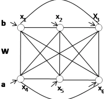
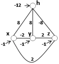
Example 1.1.1. Suppose a restricted Boltzmann machine with three visible units (x, y,z) and four hidden units (h1,h2, h3, h4), as shown in the figure below, has been trained from data, leading to a set of trained parameters as shown in the weight matrixW.

The weight matrix of this RBM is: W=               

-6.5591 -5.7882 0.8857 1.5601 -6.6418 0.7022 -6.4277 1.386 -6.5909 0.7011 0.7538 -0.39

              

The probability of a state of the visible layer being true is inversely proportional to a free energy function[53], asp(x,y,z)∝_exp(−F(x,y,_{z)) with:}

F(x,y,_z))=−

4

X

j=1

log(1+exp(w1jx+w2jy+w3jz))

(32)

the simple case where each rule is extracted from a column vector of the weight matrix, such that positive weights are converted into a positive propositionx, and negative weights into a negative proposition¬_x_{. A confidence value for the rule is}

then computed as the average of the absolute values of the weights in the column vector. For example, a vector [−6.5591 −6.6418 −6.5909] will be converted into

6.5972 :h₁ ↔ ¬_x∧ ¬_y∧ ¬_z_{. As a result, the set of confidence rules extracted from}

the weight matrixWis:

Rcon f idence=

6.5972 :h₁↔ ¬_x∧ ¬_y∧ ¬_z

2.3972 :h₂↔ ¬_x∧_y∧_z

2.6891 :h₃↔_x∧ ¬_y∧_z

1.1120 :h₄↔_x∧_y∧ ¬_z

(1.1)

wherehjis a hypothesis, andx,¬x,y,¬y,z,¬zare propositions indicating that

x=1,x=0,y=1,y=0,z=1 andz=0, respectively.

With the confidence rules, one can, for example, apply weighted MAX-SAT [112, 50] to decide on the propositions which will give the highest satisfiability of the hypotheses beingtrue. Similar reasoning can also be done in the RBM. Given the states of two of the inputs, the state of the third input will seek to maximise the joint probabilityp(x,y,z). For example, givenx = 1, y =0 thenz = 1 because

F_(x = 1,_y = 0,_z = ₁₎ = −3.263 < F_(x = 1,_y = 0,_z = ₀₎ = −2.986, implying that

p(x=1,y=0,z=1)>p(x=1,y=0,z=0).

(33)

R(_partiallow) =

6.6004 :h1↔ ¬x∧ ¬y 3.2452 :h2↔ ¬x∧y 3.6567 :h3↔x∧ ¬y 1.4730 :h4↔x∧y

R(_partialhigh) =

6.5909 :z↔ ¬_h₁

0.7011 :z↔_h₂

0.7538 :z↔_h₃

0.3900 :z↔ ¬_h₄

Now, by inspecting the symbolic part of the rules, one finds that, for example,

¬_x∧ ¬_y ↔ _h₁ _and _z ↔ ¬_h₁ _{is equivalent to} ¬_x∧ ¬_y ↔ ¬_z_{. This rule is more}

discriminative in that it represents a relationship between a group of non-target variables and a target variable.

By repeating the above process, the symbolic form of the rules extracted from the RBM are: ¬_x∧ ¬_y↔ ¬_z_,¬_x∧_y↔_z_,_x∧ ¬_y↔_z_,_x∧_y↔ ¬_z_{which represent}

the XOR functionx⊕_y↔_{z. The dataset on which the above RBM was trained was}

indeed obtained from this XOR function.

Our hypothesis is that a hierarchical representation and reasoning algorithms can provide insight into the relevance of the knowledge learned by stacks of RBMs and facilitate transfer learning, as a result.

Even though the combination of rules, as used above, will be shown in some cases not to be effective for improving prediction accuracy (particularly in complex image domains), the rules will be shown to offer a compact representation that is useful for transfer learning, i.e. to improve performance in a related or analogous domains through a better network initialisation.

(34)

weight matrixW:

R(_completelow) =

6.6004 :h₁↔(0.9937 :¬_x₎∧(1.0063 :¬_y₎

3.2452 :h2↔(1.7827 :¬x)∧(0.2164 :y) 3.6567 :h3↔(0.2422 :x)∧(1.7578 :¬y) 1.4730 :h₄↔(1.0591 :_x₎∧(0.9409 :_y₎

R(_completehigh) =

6.3909 :z↔_{(1 :}¬_h₁₎

0.7011 :z↔_{(1 :}_h₂₎

0.7538 :z↔_{(1 :}_h₃₎

0.3900 :z↔_{(1 :}¬_h₄₎

One can see that each confidence rule in a complete-model accounts for a ba-sis vector (a column vector of the weight matrix). For example, vector [−6.5591 −₆._{6418] is converted to rule 6}._{6004 :}_h₁ ↔₍₀._{9937 :} ¬_x₎∧₍₁._{0063 :}¬_y_{), where the}

rules confidence is (6.5591+6.6418)/2=6.6004, and the associated values of the two propositions¬_x_and¬_y_{are 6}.₅₅₉₁/₆.₆₀₀₄=₀._{9937 and 6}.₆₄₁₈/₆.₆₀₀₄=₁._0063,

re-spectively. Notice that the confidence values c of the confidence rules in a complete-model are the same as in the partial-complete-model of an RBM. With the confidence values of the propositions accounted for, the rules in a complete model capture exactly the column vectors of W. Therefore, in practice we only need to compute the confi-dence values of the rules and we can use the column vectors of the weight matrix as representation ofcomplete-models.

1.1.2 Knowledge Sharing and Transfer Learning

Following knowledge extraction, confidence rules can be used for reasoning, e.g. ifxis true andyis false, given conflicting rules 0.5 :h↔_x∧ ¬_y∧_zand 0.01 :_h↔

x∧ ¬_y∧ ¬_z_{, one can be more confident that}_z_{is true than it is false. Confidence rules}

(35)

improve on an otherwise random network initialisation [137, 31]. One might see this as a continuous process of using reliable knowledge provided by experts to guide the learning of new knowledge from data, as more and more data becomes available.

To enable the above knowledge refinement or, more generally, knowledge shar-ing across different (but related) domains, a system should require: source do-main(s) for which knowledge is provided; target dodo-main(s) that reuse the knowl-edge; and a transfer mechanism. For example, suppose that knowledge about a minus sign is to be used to learn new knowledge about the plus sign (as seen in an earlier example). A transfer mechanism needs to be designed with useful mapping rules. For example, a rule for a minus sign might be1:

minus↔_x₄∧_x₅∧_x₆

This rule can be used when learning new knowledge about the plus sign, as follows:

plus↔_minus∧_x₂∧_x₈

The transfer mechanism will depend on the transfer medium, i.e. the lan-guage/model in which knowledge is represented. It does not require the use of logic rules in every case, and the mapping rules can be created manually by ex-perts; however, this is a daunting task. When a mechanism automatically learns the mapping rules then this is calledtransfer learning[101, 135, 62]. In this thesis, knowledge extraction and the proposed confidence rules language will be shown useful as part of a new transfer learning algorithm, which will be shown empirically to be an effective medium for transfer learning.

1.2 Objectives

The objectives of this research are to propose, develop and evaluate a new form of knowledge representation for stacks of RBMs and to apply it to knowledge

1_{This rule uses negation by default [31]: if a proposition} _x

i does not appear in a rule then its

(36)

extraction, neural-symbolic integration and transfer learning.

Hypothesis StatementThe decomposition of complex RBM

representa-tions into logic-based proposirepresenta-tions provides an effective way of achieving

knowledge extraction, insertion and transfer between RBMs.

Specifically, this research addresses the following questions: (i) how knowledge learned by an RBM can be represented symbolically?; (ii)how learning from data and

sym-bolic knowledge can be integrated into a neural-symsym-bolic system to improve performance?;

and (iii)how symbolic knowledge can be used to improve learning from data in a different, related domain?.

We show that confidence rules offer an adequate hierarchical decomposition for the set of weight matrices of deep belief networks (DBNs). We introduce two types of rules: partial-modelsandcomplete-modelsas briefly discussed in §_{1.1. The}

idea behind partial-modelsis to offer a compact language for knowledge extraction and insertion into DBNs. With complete-models, a symbolic rule captures exactly the information in a basis vector. Such representation can be adapted to improve state-of-the-art results in transfer learning, by adapting, according to the confidence values, symbolic knowledge from a domain to data from another.

1.3 Contributions

The main contribution of this thesis is the development and evaluation of a proto-type of the Learning, Extraction and Sharing system based on deep belief networks, as described above.

(37)

A new efficient algorithm for extracting symbolic knowledge in the form of confidence rules from DBNs is introduced and evaluated. The key idea of this extraction algorithm is to decompose the weight matrix in each layer of the DBN into a set of independent symbolic elements. The extraction is shown to be use-ful by offering a compact representation, modular organisation of the rules, and support for hierarchical inference in the presence of uncertainty. This type of infer-ence is more flexible than classical logical inferinfer-ence through the use of real-valued confidence values. It is shown experimentally in image domains that confidence rules can save significant amounts of memory in comparison to RBMs while still guaranteeing performance at feature extraction tasks.

A new neural-symbolic system integrating symbolic knowledge and DBNs is proposed and evaluated. By using confidence rules as an intermediate language, we translate symbolic rules, serving as background knowledge, into a hierarchical set of weight matrices. During network training, we employ the rule inference to guide the learning. The idea of encoding symbolic knowledge into a connec-tionist system to improve learning is not new. However, this is to the best of our knowledge, the first neural-symbolic system for unsupervised learning and modu-lar reasoning using RBMs. We show on experiments using DNA sequence analysis and the MNIST handwritten digits datasets that the encoding of knowledge can help improve learning performance and inference in deep belief networks.

We propose and evaluate a method for using confidence values for representa-tion ranking. The method computes a confidence value as the mean of the absolute values of the basis vectors corresponding to a representation. We measure the usefulness of confidence values using: visualisations of the reconstructed images, classification accuracy, and mutual information. The results show that the repre-sentations with the highest confidence values capture the majority of an RBM.

(38)

can be adapted as part of the learning process at the target domain, based on the data available at the target domain. We test the algorithm by transferring representations from source RBMs trained on handwritten letters onto target RBMs trained to recognise handwritten digits. The proposed transfer algorithm is shown to outperform state-of-the-art self-taught learning and combinations of self-taught learning and RBM learning. Each confidence rule is associated with an adaptation factor which becomes a parameter for training in the target domain, allowing representations to be transformed progressively. Furthermore, the use of confidence rules offers an approach to deal with the problem of “biased sampling”. The “biased sampling” problem happens when many representations to be transferred make the learning in the target domain dependent on the source domain. By transferring only a small number of representations with high confidence values, using confidence values and mutual information, or applying dropout onto a small set of transferred representations for each batch learning in the target domain, biased sampling can be reduced. Extensive experiments confirm that the use of knowledge and adaptation factors can improve the effectiveness of the transferred representations with the target domains. Our experiments also show that transfer learning is more effective when knowledge, and not data, is transferred.

Publications

1. Son N. Tran and Artur d’Avila Garcez. Deep Belief Logic Networks. (submitted)

2. Son N. Tran and Artur d’Avila Garcez. Adaptive Transferred-profile Likelihood Learning.

(submitted)

3. Hazrat Ali, Son N. Tran, Emmanouil Benetos, Xianwei Zhou. Hybrid Representation Learning

for Speaker Recognition. (submitted)

4. Son N. Tran, Srikanth Cherla, Artur d’Avila Garcez, Tillman Weyde. Probabilistic Approach

for Relative Similarity. (in preparation)

5. Son N. Tran, Artur S. d’Avila Garcez. Efficient Representation Ranking for Transfer Learning. In International Joint Conference on Neural Network. Killarney, Ireland, 2015.

6. Hazrat Ali, Son N. Tran, Artur S. d’Avila Garcez, Tillman Weyde. Convolutional Data: Towards

Deep Audio Learning from Big Data. In 1st UCL Workshop on the Theory of Big Data. London,

UK. 2015.

7. Son N. Tran and Artur d’Avila Garcez. Low-cost Representation for Restricted Boltzmann

Machine.In 21st International Conference on Neural Information Processing. Kunching, Malaysia,

(39)

8. Thanh Vu, Dawei Song, Alistair Willis, Son N. Tran. Improving Search Personalisation with

Dynamic Group Formation.In SiGIR. Australia, 2014.

9. Son N. Tran, Emmanouil Benetos and Artur d’Avila Garcez. Learning Motion-Difference Fea-tures using Gaussian Restricted Boltzmann Machines for Efficient Human Action Recognition. In International Joint Conference on Neural Network. Beijing, China, 2014.

10. Son N. Tran, Daniel Wolff, Tillman Weyde, and Artur d’Avila Garcez. Feature Preprocessing with Restricted Boltzmann Machine for Music Similarity Learning.In Audio Engineering Society

53rd conference on Semantic Audio. London, UK, 2014. (Winner of Reproducible Prizes).

11. Hazrat Ali, Artur d’Avila Garcez, Son N. Tran, Xianwei Zhou. Hybrid Features Combination

for Audio Data Classification. In Machine Learning and Data Analytics Symposium, 3-4 March,

Doha, Qatar, 2014.

12. Son N. Tran and Artur d’Avila Garcez. Knowledge Extraction from Deep Belief Networks

for Images.In IJCAI-2013 Workshop on Neural-Symbolic Learning and Reasoning. Beijing, China,

2013.

13. Son Tran and Artur Garcez. Logic Extraction from Deep Belief Networks. In ICML2012

Representation Learning Workshop. Edinburgh,UK, July 2012

Software and code

Link: https://github.com/sFunzi/

1. RepDeepLearn: Implementation of representation/deep learning and reason-ing models such as restricted Boltzmann machines (RBMs), Auto Encoders, Non-negative Matrix Factorization, Sparsity, deep belief networks (DBNs), deep Boltzmann machines (DBMs), Neural Networks

2. ConfidenceLogic: Knowledge Extraction from RBMs and DBNs

3. Motion-Difference: Action recognition

4. RelSim: Relative similarity models, tested on music data

5. ATPL: Extraction and transfer of representation from learned RBMs

1.4 Organisation of the Thesis

(40)

contributions of the work.

Chapter 2introduces the deep models used forLES: Learning-Extraction-Sharing. We review the theory of representation learning, RBMs and deep learning using unsupervised models. We illustrate the use of stacks of RBMs in a range of ap-plications in music similarity, action recognition, speaker recognition and melody modelling. We review the related work on knowledge-based neural networks, knowledge extraction and transfer learning.

Chapter 3 reviews the related work on Penalty Logic and extends Pinkas re-sults to DBNs by showing that propositional calculus is equivalent to minimising a DBNs energy function. We observe that the signs of the weights already represent the logical propositions, which will serve as the basis for an efficient extraction algorithm. We introduce the concept of confidence rules formally and show that confidence rules can be approximated by training a DBN. This indicates that the extraction of confidence rules from DBNs is promising, which will then be investi-gated empirically.

In Chapter 4, we introduce the concepts of partial-modelsandcomplete-models formally. We present an algorithm for the extraction ofpartial-modelsfrom RBMs and DBNs. We then empirically investigate the effectiveness of the extracted partial-models in terms of representation and inference. Based on the results, we also propose an encoding algorithm to integrate symbolic background knowledge and learning in DBNs.

In Chapter 5 we investigate the use of confidence values for representation ranking and transfer learning. The representations are seen as a set of complete-modelsextracted from a domain to be ranked and transferred to improve learning in another domain. We show that confidence values can be used to rank the representations which are then to be transferred.

(41)

target domain. Experimental results are analysed extensively, indicating that the proposed transfer method can improve on the state-of-the-art.

(42)

Background

Recent research has shown that an emerging technique called deep learning can be effective in vision, audio, and text domains. Furthermore, with an effective layer-wise unsupervised learning, a deep network can learn a hierarchy of concepts from data. This chapter reviews deep networks - its building block restricted Boltzmann machines and deep belief networks - and applications using unsupervised learning. It also reviews related work on knowledge-based neural networks and transfer learning.

2.1 The Importance of Unsupervised Learning in Deep

Learn-ing

Deep beliefs networks are one among many machine learning models which have been categorised as “deep networks” [64, 75, 54, 11, 12, 119, 120, 122, 143]. The term “deep network” usually refers to a connectionist system which has many hidden layers. An early deep network model was the multi-layer artificial neural network (ANN) [64, 65]. However, training deep ANNs is not easy due to a problem called “vanishing/exploding gradient” with the back-propagation algorithm [59]. This problem can be alleviated through unsupervised layer-wise learning [122].

With more attention paid to deep learning and further study of unsupervised layer-wise learning [38, 56, 132], recent research indicates that it is possible to train a

(43)

deep network purely by supervised algorithms using rectified linear units [93, 45]. While supervised deep learning is shown to be adequate to the effective learning of input-output mappings given large amounts of data, some researchers remain concerned about the role of unsupervised learning for the following reasons.

First, it has been shown through theoretical and experimental results that su-pervised learning is not always preferred over unsusu-pervised learning [97]. In particular, even though unsupervised learning tends to achieve higher error (lower accuracy) it can converge faster than supervised learning in many cases. In deep learning, a well known experiment in the Google Brain project showed that it is possible to train a classifier without providing any label by stacking shallow models one on top of another [73].

Second, Bottou has raised a question about “a new path to AI” in that we can “algebraically enrich the set of manipulations applicable to training systems, and build reasoning capabilities from the ground up” [17]. Especially, in the Nature Review paper [143], Lecun, Bengio and Hinton have expressed their expectation that unsupervised learning in deep networks should become more important. This has been echoed by most of the panellists in the Panel Discussion at ICML 2015 Deep Learning workshop1.

In this thesis we focus on DBNs, unsupervised models of deep learning created by stacking restricted Boltzmann machines on top of each other [54], as specified below.

2.2 Energy-based Connectionist Systems

Connectionist systems normally refer to a set of models made by interconnected networks of neurons (or units) [124, 51]. An energy based connectionist system (ECS)Nis a neural network with bidirectional connections which is characterised by an energy function:

EN(x)=−

X

∀_i∀_j>_i

fi j(x)−

X

∀_i

gi(x) (2.1)

(44)

where fi j and gi are potential functions for the state x of the model. There exist

different types of ECSs depending on how this function is defined. This also characterises a probability distribution of a model as:

p(x)= e

−_E₍_x)/_T

Z (2.2)

whereTis the temperature andZ=P xe

−_E₍_x)/_T

is a partition function.

The probability of a unitibeing activated (xi=1) given the states of some other

unitsxj⊂\_iis:

P(xi|xj⊂\_i)= X

xk,j

p(xi =1,xk,j|xj⊂\i) (2.3)

wherexj⊂\_i denotes a subset of the units which does not containxi,x\_i denotes all

the units in the model exceptxi, andxk,jis another subset such thatx\i =xj⊂\i∪xk,j

and∅=xj⊂\_i∩x_k_,_j.

In what follows, we recall three well-known instances of the above model: Hopfield networks, Boltzmann machines and restricted Boltzmann machines, all belonging to the same family of potential functions fi j(x) =wi jxixjandgi(x)=sixi,

wherewi jis the connection weight between unitsxiandxj, andsiis a bias forxi. If

functionfconsists of the product of more than two units, e.gfi jk(x)=wi jkxixjxk, then

the model is called “higher-order”. These models can be seen as generative models [83, 97, 10] which represent a joint probability between the variables and which can be trained by unsupervised algorithms. The term “generative” is used in this context to distinguish from “discriminative” models which represent a conditional probability of the data given a label variable [97, 70]. Discriminative models are usually trained by supervised learning algorithms.

(45)

2.2.1 Hopfield Networks

A Hopfield network [61] is a neural network with recurrent connections. The state of each unit (or neuron) can be 0 or 1, where state 0 indicates “not firing” and state 1 indicates “firing”. One may see a Hopfield network as an energy-based connectionist system, with temperatureT=0 [57], and therefore the inference rule in Eq. 2.3 becomes deterministic.

xi=

        

1 if P

jwi jxj+si>0;

0 otherwise ;

(2.4)

[image:45.595.211.383.434.598.2]

Starting from an initial state x(0), the model can iteratively update to a final state that minimises the function in Eq. 2.1. It can also be seen as a Markov chain of a symmetric connectionist system with zero temperature. This property makes Hopfield networks able to act as associative memory systems where each memory state is a local minimum of the energy function. An example of Hopfield network is shown in Figure 2.1.

Figure 2.1: A Hopfield network (s={_a,_b}_).

2.2.2 Boltzmann machines

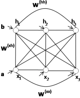
Boltzmann machines (BMs) [57] are energy-based connectionist systems in which the temperatureT ,0. We useIandJ to denote the number of observed (visible)

(46)

network, the weight matrix of a Boltzmann machine is symmetric, but it can be expressed in terms ofw(_{i j}xh),w(_iixx0 ),w

(hh)

j j0 to denote, respectively, the connection weight

between unit x in the visible layer and unit h in the hidden layer, the weight between two units in the visible layer, and the weight between two units in the hidden layer, as shown in Figure 2.2. We also useai andbj to denote the biases of visible unit i

and hidden unit j. The energy function of a Boltzmann machine then becomes:

EBM(x,h)=− I,J

X

i,j

w(_{i j}xh)xihj− I,I

X

i,i0

>i

w(_iixx0 )xixi0− J,J

X

j,j0

>j

w(_{j j}hh0)hjhj0 − I

X

i

aixi− J

X

j

bjhj (2.5)

A Boltzmann machine can be trained by maximising the log-likelihood:

MinimiseL_N =_log_p(D₎ _(2.6)

whereD_{is the observed data from a domain. Inference of the state of a unit in one}

layer given the state of the other layer is intractable if the number of units in this layer is large. Normally, then, one can use Gibbs sampling [23] over the network to get data samples from the marginal distributionp(x)=P

hp(x,h) until equilibrium

[image:46.595.211.383.455.665.2]

is reached.

Figure 2.2: A Boltzmann machine.

(47)

are needed for approximating the gradients [94, 44]. However, MCMC methods are usually computationally expensive and their convergence time is hard to predict. In order to reduce the inference time in the training, one may use variational methods [67] to approximate the states of the units.

The gradient of the log-likelihood function in Eq. 2.6 is:

∇θ=_Eh∂EBM(x,h)

∂θ

i

h|_x−E

h∂E_BM(x,h)

∂θ

i

x,h (2.7)

The first term gives an expectation of the gradient over the conditional dis-tribution p(h|_x_{), and the second term, the expectation over the joint distribution}

p(x,h). In Boltzmann machines, these expectations are both intractable. To learn the model, a more recent and popular alternative to variational methods, is the Contrastive Divergence (CD) algorithm [52]. CD is an efficient algorithm, to ap-proximate good parameters for the model. The CD algorithm apap-proximates the negative log-likelihood by minimising the difference of the two Kullback-Leibler divergences [69, 52].

KL(p(xD)kp(x;θ)_k)−KL(p(x;θ)_kkp(x;θ)∞) (2.8)

wherep(xD) is the data distribution,p(x;θ)_kandp(x;θ)∞are the model distribution

after a k step Gibbs sampling and the model distribution at equilibrium state, respectively.

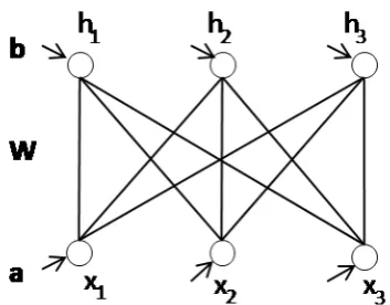
2.2.3 Restricted Boltzmann Machines

A restricted Boltzmann machine (RBM) withIvisible units andJhidden units has energy function:

ERBM(x,h)=− I,J

X

i,j

wi jxihj− I

X

i

aixi− J

X

j

bjhj (2.9)

(48)

[image:48.595.209.386.75.213.2]

Figure 2.3: A restricted Boltzmann machine.

constraint, the calculation of the probability of a unit in a layer being activated (i.e. =1) given the state of the other layer becomes tractable :

P(xi|h)=σ(

X

j

wi jhj+ai)

P(hj|x)=σ(

X

i

wi jxi+bj)

(2.10)

where σ(x) = 1/(1+exp(−_{x)) is a sigmoid function. The gradient of the}

log-likelihood w.r.t the RBMs parameters is:

∇_w_{i j}=h_x_i_P(h_j|_x₎i₀− h_x_i_P(h_j|_x₎i_∞ ∇_a_i=h_x_ii₀− h_x_ii_∞

∇_b_j =h_P(h_j|_x₎i₀− h_P(h_j|_x₎i_∞

(2.11)

where h.i₀ _{represents the empirical expectation over a data distribution and}h.i_∞

represents the expectation over model distribution (See Appendix B.1 for the proof). Again, we can use CD to efficiently approximate the parameters such that∇_w_{i j} = h_x_i_P(h_j|_x₎i₀− h_x_i_P(h_j|_x₎i_k_{, where}_k_{is a finite (small) number of Gibbs sampling. In}

many casesk=1 works surprisingly well.

(49)

weight PCD [134] combines CD and PCD by running two algorithms in parallel and averaging the updates of the weights.

In case there exists label y, inference can be done through Gibbs sampling, i.e. by initially setting y = 0.5 and reconstructing the value of y after inferring the state of the hidden layer. Gibbs sampling is an approximation method which is necessary because of the intractable partition function. Fortunately, the conditional distributionp(y=o|_x_{) is tractable. For example, multiple class label can be encoded}

as a one-hot vector wherey=ois presented by setting the unitoas 1 and the other units as 0s, and the conditional distribution is computed as:

p(y=o|_x₎= e

lboQ

j(1+ex >

wj+uo j+bj₎

P

o0elbo0Q_j(1+ex

>

wj+uo0_j+b_j

) (2.12)

wherewjare the column vectors of the weight matrixWbetween the input layer

and the hidden layer,uo jare the elements in the weight matrixUbetween the label

layer and the hidden layer, bj andlbo are biases for the units in the hidden layer

and the label layer respectively.

2.2.4 Deep Belief Networks

A DBN is constructed by stacking several RBMs one on top of another [54]. The stacking is necessitated because an RBM may not be able to learn the data distribu-tion, but an improvement can be achieved by adding one or more RBMs on top of it so that the latent variables of each RBM become the input variables of the next RBM in the stack [95, 54]. Learning can be done in sequence, i.e by training each RBM from the bottom up one at a time. This is called “unsupervised layer-wise learning” [54, 11]. Although there is no guarantee that this process will produce the improvement in learning performance mentioned above, the use of a stack of RBMs with different sizes of hidden layers trained by Contrastive Divergence has been shown useful at learning hierarchical representations [79, 78, 91, 73, 38] or for initialising a classifier [54, 11, 119].

(50)

Figure 2.4 shows a DBN trained on the MNIST handwritten digits dataset. For each hidden unit, a visualisation can be generated by setting the unit to 1 while setting all the other units in the same layer to 0, and performing downward inference to the bottom (input) layer. In this example, the different levels of representation can be visualised: in the first hidden layer, the units tend to capture low level, local information such as curves. In the second hidden layer, the units capture a higher-level of abstractions such as shapes. And finally, in the third hidden layer the units seem to represent the highest level of abstraction, i.e. the classes of the digits in the dataset.

After layer-wise training one can apply bottom-up inference to infer the state of the top layer which may include the label. One can also use the higher-level features as input to train a classifier [111, 79, 78, 73] or apply fine-tuning [54, 11, 119]. In this thesis, fine-tuning is not used because we are interested in investigating the modular unsupervised training of the networks. Instead, the raw input data is mapped onto the values of higher-level features (e.g. the values of the neurons in the third hidden layer of Figure 2.4). Such features are then provided separately as input to a classifier, together with labels, for the purpose of supervised learning; in our experiments, Support Vector Machines (SVMs) are used as classifier2_{. Furthermore,} in order to evaluate the rule inference we will compare it with bottom-up inference in DBNs (§_4.3).

2.3 Applications

An interesting property of deep networks is the unsupervised modular learning illustrated in Figure 2.4. In this section, we review a number of applications of this approach in different domains. More information about these applications can be found in Appendix A.

We have applied an RBM to learn features that can improve standard music similarity models (see §_{A.1 for more details). After training, the probability}

distri-bution of the hidden layer given a state of the visible layer, is used as input to an

2_{We use SVMs because it has a few number of hyper-parameters which is convenient for model}

(51)

SVM for classification [125]. The use of the features produces a better classification performance in the SVM than the original data made of audio signals and texts (user tagging). The features produced by the RBM also produce a better classification performance than standard PCA features [105].

In the case of audio data, RBMs also outperform handcrafted features such as Mel-frequency Cepstral Coefficients (MFCC) [145] in a speaker recognition task (see §_{A.3 for more details). If we combine the features from di}ff_{erent layers of a}

DBN and MFCC features the performance of the classifier can be further improved.

Features from RBMs can also be learned to help improve an action recognition task, as detailed in §_{A.2. The filter bases learned from the motion-di}ff_erence

Weizmann dataset and KTH dataset are visualised in Figure 2.5. Differently from other approaches which seek to learn local Gabor filters from the image frames [142, 74], RBMs seem to learn movement patterns as visualised as pairs of black and white lines and curves. In addition, the use of RBMs offers an improvement of prediction accuracy and learning efficiency.

Similar results can also be achieved from audio signals, for example in an application of RBMs to a music genre classification task [4]. In this application, based on the idea of convolution in unsupervised learning [78], Figure 2.6 shows representations obtained from RBMs trained on the spectrograms of different types of music. Each sub-figure corresponds to a spectrogram in a specific duration of time characterising six music genres.

(52)

2.4 Knowledge Extraction

We have seen that representation learning can be effective in different domains. This indicates a promising use for knowledge extraction and sharing from RBMs and DBNs. The study of knowledge extraction from such networks is new. As far as we know, we have been the first to propose this challenge [126, 138] building on the work of others on knowledge extraction from Hopfield networks, Boltzmann machines and Recurrent Temporal RBMs [109, 36]. In this Section, we review several knowledge extraction techniques including the above, and discuss how they differ from our proposal.

A feed-forward neural network (NN) is a multi-layer connectionist system [114, 87, 5], which is different from DBNs, as the term is used in this thesis. The NNs are representations of input-output mapping functions while DBNs are representations of joint distributions. Research has shown that using a layer-wise learning for parameter initialisation in NNs can help achieve better performance in NNs [55, 54, 11]. Nevertheless, as already mentioned, in this thesis we are concerned with layer-wise unsupervised learning.

Extraction of symbolic knowledge from neural networks is critical for neural-symbolic integration [32, 48], where the common approach is to learn from data and background knowledge using NNs and to extract a revised symbolic knowledge from the trained networks. Most of the work on knowledge extraction has been focused on extraction algorithms applicable to neural networks trained using su-pervised learning, notably back-propagation. Towell and Shavlik [136] propose the M-of-N (MofN) method of rule extraction from a trained neural network. A MofN rule is expressed ash←_x₁∧_x₂∧...∧_x_N_{, meaning ”If any M out of N propositions}

in the body of the rule are true thenhis true”. For example, withh ← _x₁ ∧_x₂∧_x₃_,

the 2of3 rule means any assignment{_x1,_x₂}_,{_x2,_x₃}_or{_x1,_x₃}_{can imply}_h_{. Another}