Comment on "Nonlinear eigenvalue problems"

City, University of London Institutional Repository

Citation

:

Kerr, O. (2014). Comment on "Nonlinear eigenvalue problems". Journal of

Physics A: Mathematical and Theoretical, 47, p. 368001. doi:

10.1088/1751-8113/47/36/368001

This is the accepted version of the paper.

This version of the publication may differ from the final published

version.

Permanent repository link:

http://openaccess.city.ac.uk/3829/

Link to published version

:

http://dx.doi.org/10.1088/1751-8113/47/36/368001

Copyright and reuse:

City Research Online aims to make research

outputs of City, University of London available to a wider audience.

Copyright and Moral Rights remain with the author(s) and/or copyright

holders. URLs from City Research Online may be freely distributed and

linked to.

City Research Online:

http://openaccess.city.ac.uk/

[email protected]

On “Nonlinear eigenvalue problems”

Oliver S. Kerr

Department of Mathematics, City University London,

Northampton Square, London, EC1V 0HB, U.K.

Abstract

The asymptotic behaviour of solutions to y0(x) = cos[πxy(x)] was investigated by Bender, Fring and Komijani [2]. They found, for example, a relation between the initial value y(0) = a and the number of maxima that the solution exhibited. We present an alternative derivation of the asymptotic results that looks at the solutions in the regions x < y and x > y, and confirms the behaviour found previously for larger values ofa. This method uses the small amplitude and high frequency of the oscillatory behaviour in the regionx < y.

PACS numbers: 02.30.Hq, 02.30.Mv, 02.60.Cb

1 Introduction 2

1

Introduction

In a recent paper by Bender, Fring and Komijani [2] a detailed asymptotic analysis of the nonlinear initial-value problem

y0(x) = cos[πxy(x)], y(0) =a (1)

was presented which focused on the solutions forx≥0. They showed that for a >0 solutions could be split into classes depending on the initial conditions such that solution with an−1 < a < an displayed an oscillatory region with n maxima before

decaying monotonically to zero. They then found the result that as n → ∞, an ∼

25/6√_{n. The purpose of this paper is to present an alternative derivation of this result}

that may be simpler to adapt to analogous problems.

2

Outline

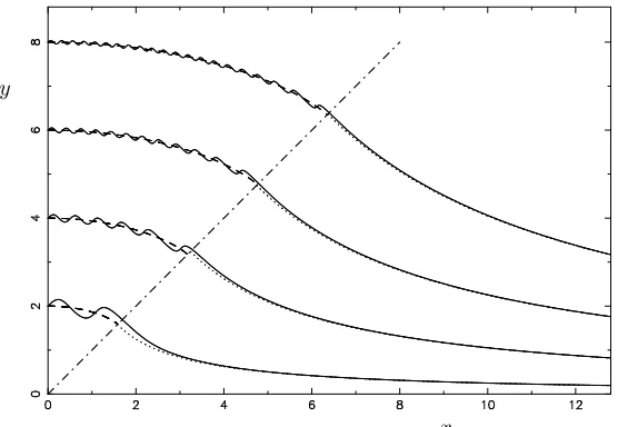
The typical behaviour of solutions to (1) is shown by the solid lines in figure 1. There is an initial oscillatory phase where the frequency increases and the amplitude decreases as the initial value,y(0), increases. These oscillatory solutions drift downwards until they undergo a transition to monotonic decay towards the horizontal axis.

y

x

Fig. 1: Plots of solutions to (1) with y(0) = 2, 4,6,8. The dotted lines in

x > y show the curvesxy =C to which these converge asymptotically asx→ ∞. The dashed lines inx < ygive the estimate of the mean path of the oscillatory part of these curves.

3 Solutions in the regionx > y 3

in figure 2. If we consider lines wherexy = 2n then solutions will have gradient 1

y

x x=y

xy= 2n xy= 2n+1

2

xy= 2n+ 1

xy= 2n+3₂

xy= 2n+ 2

xy= 2n+5₂

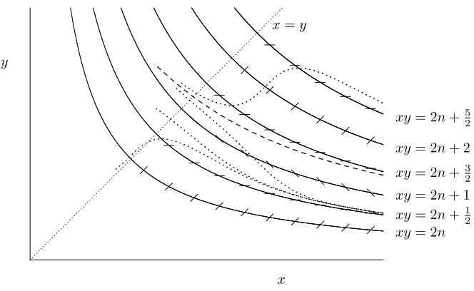
Fig. 2: Schematic plot for solutions in the regionx > yand the influences of the

lines of formxy=C. The dotted lines show the trajectories of various solutions, while the dashed line shows the path of the separatrix dividing solutions that converge to xy = 2n+ 1/2 from those that converge to

xy= 2n+ 5/2.

where they intersect these lines, similarly whenxy= 2n+ 1 they will intersect with gradient−1, and whenxy= 2n±1/2 they will intersect with gradient 0. The gradients of the solutions will have gradients with magnitude at most 1, while the linesxy=c

for constantsc have gradients greater than 1 in magnitude forx < y, and less than 1 forx > y. In the region x < y solutions must cross the linesxy =cfrom left to right, with a maximum each time it crosses a linexy= 2n+1₂,n= 1,2,3, . . .. In the regionx > ythis restriction no longer holds. This results in the solutions having intrinsically different behaviour above and below the linex=y.

3

Solutions in the region

x > y

The behaviour of solutions in this area is addressed by problem 4.13 in the book by Bender and Orszag [1]. Any solution that enters a region 2n+1

2 ≤xy≤2n+ 1 is

trapped in this region asxincreases as the gradient of a solution on the lower boundary is 0, and on the upper boundary is−1. Indeed, in such a region any solution that is initially above a linexy= 2n+1

2+will have a negative gradient of magnitude greater

than sinπand so must eventually pass belowxy= 2n+1₂+, whose gradient tends to zero asx→ ∞. Thus all solutions in this region asymptote to the linesxy= 2n+1

4 Solutions in the regionx < y 4

All solutions in the region 2n−1

2 < xy <2n+ 1

2 will have positive gradients and

so will pass into the region 2n+ 1

2 ≤ xy ≤ 2n+ 1 from below, and will have one

maximum in the regionx > y.

As Benderet al.showed, there is one solution in the region 2n+ 1< xy <2n+3 2

that stays in this region. Solutions initially below this curve will pass into the region the curve gradients of any solution 2n+ 1

2 ≤xy ≤2n+ 1 and remain there, while

those above it will end up in the region 2n+5

2 ≤xy≤2n+ 3. This curve is indicated

by the dashed line in figure 2. By a similar argument to that given previously it can be shown that these seperatrices tend towards their asymptotesxy= 2n+ 3/2 from below. We will denote the point where the separatrix crosses the line asx=y=bn,

and hence (2n+ 1)1/2_{< b}

n<(2n+ 3/2)1/2.

Clearly, any solution that ends up just above the curve xy = 2n+1₂ will have crossed n lines given by xy = 1

2, 5 2,

9

2, . . .and so will have n maxima. Hence any

solution that crosses the linex=ywithbn−1< x=y < bnwill havenmaxima.

4

Solutions in the region

x < y

For large values ofy the solution y(x) will tend to oscillate quickly with small am-plitude. What we are going to do is exploit this to seek the behaviour of the local average of the solution. A schematic diagram of the behaviour of an enlarged section of the trajectory is shown in figure 3.

Locally we can approximate the lines of constant x as parallel lines, as shown in figure 3. and so we can determine the leading order behaviour by looking at the

y

x

Fig. 3: Diagram showing the local approximation to lines ofxy=C as parallel

4 Solutions in the regionx < y 5

solutions to

y0(x) = cos[ω(x+αy)], 0< α <1. (2) If we let

X=x+αy (3)

then

dy

dX =

dy

dx

1 +αd_dy_x =

cosωX

1 +αcosωX (4)

We are interested in the average change inyover a cycle, say ∆y, which corresponds toX changing by 2π/ω. This is given by

∆y=

Z 2π/ω

0

cosωX

1 +αcosωXdX. (5)

This can be evaluated by, say, converting the integral into a complex contour integral about the unit circle centred on the origin,C, by settingz=eiωX to give

∆y= 1

iω

I

C

z2+ 1

z(αz2_{+ 2z+α)}dz (6)

Evaluating this using residues gives

∆y=2π

ω

1

α−

1

α√1−α2

. (7)

AsX changes by ∆X= 2π/ω, this gives the average slope of the path to be

∆y

∆X =

1

α−

1

α√1−α2, (8)

which is independent of the frequency of the oscillations. At leading order we can use this to give the slope of the mean line

dy

dX =

1

α−

1

α√1−α2. (9)

whereα changes on a scale longer than that of the oscillations. Converting back to

x–ycoordinates gives dy

dx =

dy

dX

1−α_dd_Xy =

√

1−α2₋₁

α . (10)

Up to now we have not specified what αis. It is determined by the hyperbolas

xy=c. On such curves

dy

dx=− c x2 =−

y

x. (11)

Since the gradient of the linesx+αy=cis−1/α, we findα=x/yand so the equation for the slope of the average curve is given by

dy

dx=

r _y

x

2

−1−y

x. (12)

This has solutions

5 Conclusions 6

The solution curves meet the linex=ywhen

x=y= 2−1/3y(0) (14) These curves are shown by the dashed lines in figure 1, showing good agreement even for these moderate values ofy(0).

Theanof Benderet al. are the values ofy(0) which correspond to thebn, and so

to leading order

an≈21/3bn= 21/3 21/2n1/2+O(n−1/2)= 25/6n1/2+O(n−1/2), (15)

giving the same result as found by Benderet al..

5

Conclusions

We have presented here alternative derivation of the results of Bender, Fring and Komijani [2]. Their derivation could be considered to be more mathematically elegant, and for this problem easier to obtain higher order asymptotic behaviour than it would be by the methods presented here. However, the alternative approach adopted here obtains the same leading order behaviour in a way that is possibly more adaptable to analogous problems, and where the leading order asymptotic behaviour is sufficient.

References

[1] C. M. Bender and S. A. Orszag. Advanced Mathematical Methods for Scientists and Engineers. McGraw-Hill, New York, NY, USA, 1978.