Nonlinear eigenvalue problems

City, University of London Institutional Repository

Citation

:

This is the submitted version of the paper.

This version of the publication may differ from the final published

version.

Permanent repository link:

Link to published version

:

Copyright and reuse:

City Research Online aims to make research

outputs of City, University of London available to a wider audience.

Copyright and Moral Rights remain with the author(s) and/or copyright

holders. URLs from City Research Online may be freely distributed and

linked to.

Carl M. Bendera,b,∗ Andreas Fringb,† and Javad Komijania‡

a_{Department of Physics, Washington University, St. Louis, MO 63130, USA} b_{Department of Mathematical Science, City University London,}

Northampton Square, London EC1V 0HB, UK

(Dated: January 24, 2014)

This paper presents a detailed asymptotic study of the nonlinear differential equation

y0(x) = cos[πxy(x)] subject to the initial condition y(0) = a. Although the differential equation is nonlinear, the solutions to this initial-value problem bear a striking resemblance to solutions to the time-independent Schr¨odinger eigenvalue problem. As xincreases from

x= 0, y(x) oscillates and thus resembles a quantum wave function in a classically allowed region. At a critical valuex=xcrit, wherexcrit depends ona, the solution y(x) undergoes

a transition; the oscillations abruptly cease andy(x) decays to 0 monotonically asx→ ∞. This transition resembles the transition in a wave function that occurs at a turning point as one enters the classically forbidden region. Furthermore, the initial conditionafalls into discrete classes; in thenth class of initial conditions an−1< a < an (n= 1,2,3, . . .), y(x) exhibits exactlynmaxima in the oscillatory region. The boundariesan of these classes are the analogs of quantum-mechanical eigenvalues. An asymptotic calculation of an for large nis analogous to a high-energy semiclassical (WKB) calculation of eigenvalues in quantum mechanics. The principal result of this paper is that asn→ ∞,an∼A

√

n, whereA= 25/6_.

Numerical analysis reveals that the first Painlev´e transcendent has an eigenvalue structure that is quite similar to that of the equationy0(x) = cos[πxy(x)] and that thenth eigenvalue grows withnlike a constant timesn3/5 _{as n→ ∞. Finally, it is noted that the constantA}

is numerically very close to the lower bound on the power-series constantP in the theory of complex variables, which is associated with the asymptotic behavior of zeros of partial sums of Taylor series.

PACS numbers: 02.30.Hq, 02.30.Mv, 02.60.Cb

I. INTRODUCTION

This paper presents a detailed asymptotic analysis of the nonlinear initial-value problem

y0(x) = cos[πxy(x)], y(0) =a. (1)

This remarkable and deceptively simple looking differential equation was given as an exercise in the text by Bender and Orszag [1]. Since then, it and closely related differential equations have arisen in a number of physical contexts involving the complex extension of quantum-mechanical probability [2, 3] and the structure of gravitational inspirals [4]. We will see that the properties of solutions to this equation are strongly analogous to those of the time-independent Schr¨odinger eigenvalue problem.

Recall that the Schr¨odinger eigenvalue problem has the general form

−ψ00(x) +V(x)ψ(x) =Eψ(x), ψ(±∞) = 0, (2)

∗

Electronic address: cmb@wustl.edu

†

Electronic address: a.fring@city.ac.uk

‡

Electronic address: jkomijani@physics.wustl.edu

whereEis the eigenvalue. For simplicity, we assume that the potentialV(x) has one local minimum and rises monotonically to ∞ as x → ±∞. In general this eigenvalue problem is not analytically solvable except for special potentials [such as the harmonic oscillator potentialV(x) =x2]. How-ever, it is possible to find the large-n asymptotic behavior of the nth eigenvalue En by using semiclassical (WKB) analysis. To leading order the large-nasymptotic behavior of the eigenvalues of the two-turning-point problem may be obtained from the Bohr-Sommerfeld condition

Z x2 x1

dxpEn−V(x)∼(n+ 1/2)π (n→ ∞), (3)

where the turning pointsx1 andx2are real roots of the equationV(x) =En. This WKB condition determines the eigenvalues implicitly for large n. As an example, for the anharmonic potential

V(x) =x4 the large-nasymptotic behavior of the eigenvalues is [5]

En∼Bn4/3 (n→ ∞), (4)

where the constantB is given by B = 3Γ(3/4)√π/Γ(1/4).

The quantum eigenfunctionsψ(x) exhibit several well known characteristic features. In the clas-sically allowed region between the turning points (x1 < x < x2), the eigenfunctions are oscillatory

and the eigenfunction corresponding toEnhasnnodes. In the classically-forbidden regionsx > x2

and x < x1 the eigenfunctions decay exponentially and monotonically to zero as|x| → ∞. Thus,

at the turning points the behavior of the eigenfunctions changes abruptly from rapid oscillation to smooth exponential decay.

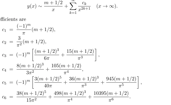
The solutions y(x) to the nonlinear differential equation (1) have many features in common with the solutions ψ(x) to the Schr¨odinger equation (2). For any choice of y(0) = a the initial slopey0(0) is 1. Asxincreases from 0,y(x) oscillates as shown in Fig. 1. This regime of oscillation is analogous to a classically allowed region in quantum mechanics. Note that the number of maxima of the function y(x) in the oscillatory region increases as y(0) increases. With increasing

x the oscillations abruptly cease, and as x → ∞ the function y(x) then decays smoothly and monotonically to 0. This kind of behavior resembles that ofψ(x) in a classically forbidden region. Figure 1 reveals that in the decaying regime the curves merge into quantized bundles. This large-x asymptotic behavior of y(x) can be explained by using elementary asymptotic analysis. If we seek an asymptotic behavior of the form y(x) ∼c/x(x → ∞) and substitute this ansatz into (1), we find thatc=m+ 1/2 (m= 0,1,2,3, . . .). This is just theleading term in the asymptotic expansion of y(x) for large x. The full series has the form

y(x)∼ m+ 1/2

x +

∞

X

k=1

ck

x2k+1 (x→ ∞). (5)

The first few coefficients are

c1 =

(−1)m

π (m+ 1/2),

c2 =

3

π2(m+ 1/2),

c3 = (−1)m

(m+ 1/2)3

6π +

15(m+ 1/2)

π3

,

c4 =

8(m+ 1/2)3 3π2 +

105(m+ 1/2)

π4 ,

c5 = (−1)m

3(m+ 1/2)5 40π +

36(m+ 1/2)3

π3 +

945(m+ 1/2)

π5

,

c6 =

38(m+ 1/2)5 15π2 +

498(m+ 1/2)3

π4 +

10395(m+ 1/2)

5 10 15 20 x 2

4 6 8 10

yHxL

FIG. 1: Numerical solutions y(x) to (1) for 0 ≤ x ≤ 24 with initial conditions y(0) = 0.2k for k = 1, 2,3, . . . ,50. The solutions initially oscillate but abruptly become smoothly and monotonically decaying. In the decaying regime the solutions merge into discrete quantized bundles.

A. Hyperasymptotic analysis

A close look at Fig. 1 shows a surprising result: Half of the predicted large-x asymptotic behaviors in (5) appear to be missing. The bundles of curves shown in Fig. 1 correspond only toeven

values ofm. To explain what has happened to the odd-m bundles, we perform a hyperasymptotic analysis (asymptotics beyond all orders) [6]. Let y1(x) and y2(x) represent two different curves

in the mth bundle. Even though they are different curves they have exactly the same asymptotic approximation as given in (5). Then Y(x)≡y1(x)−y2(x) satisfies the differential equation

Y0(x) = cos[πxy1(x)]−cos[πxy2(x)]

= −2 sin1₂πxy1(x) +1₂πxy2(x)

sin1₂πxy1(x)−1₂πxy2(x)

∼ −2 sinπ m+1₂sin1₂πxY(x) (x→ ∞)

∼ −(−1)mπxY(x) (x→ ∞). (7)

Thus, we conclude that

Y(x)∼Kexp−(−1)mπx2 (x→ ∞), (8)

where K is an arbitrary constant. This calculation shows that while two different curves in the same bundle have the same asymptotic expansion for largex, they differ by an exponentially small amount. This result explains why no arbitrary constant appears in the asymptotic expansion (5); the arbitrary constant appears in the beyond-all-orders hyperasymptotic (exponentially small) correction to this asymptotic series.

and discrete curve, called a separatrix, for the case of odd m. The nth separatrix, whose large-x

asymptotic behavior is (2n−1/2)/x (n = 1,2,3, . . .), is unstable for increasing x; that is, as x

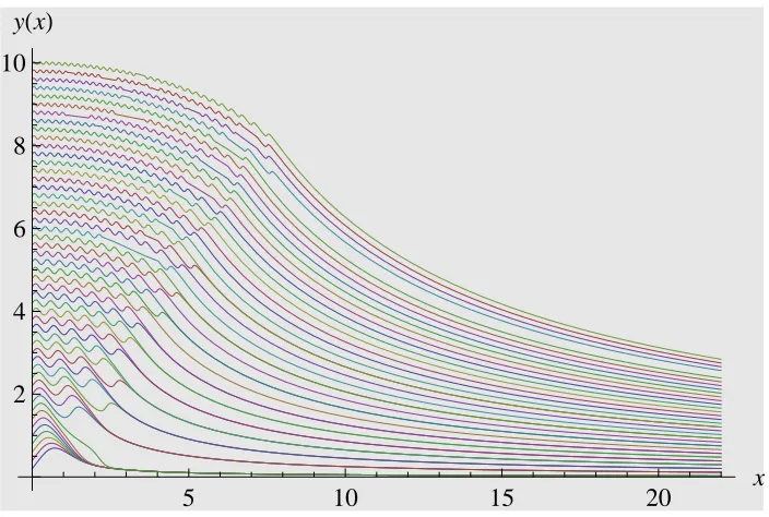
increases, nearby curvesy(x) veer away from it and become part of the bundles above or below the separatrix. This explains why there are no curves shown in Fig. 1 whenm is odd. Ten separatrix curves are shown in Fig. 2.

0 1 2 3 4 5 6

−3 −2 −1 0 1 2 3 4

x

y

FIG. 2: Numerical solutions to (1) showing ten separatrix curves, which cross theyaxis ata−3=−3.231360,

a−2 = −2.698369, a−1 = −2.032651, a0 = −1.016702, a1 = 1.602573, a2 = 2.388358, a3 = 2.976682,

a4= 3.467542,a5= 3.897484, anda6= 4.284674.

While the separatrix curves are unstable for increasing x, they are stable for decreasing x and thus it is numerically easy to trace these curves backward from large values of x down to x = 0. We treat the discrete point an (n= 1,2,3, . . .) at which the nth separatrix crosses the y axis as an eigenvalue. The curves y(x), whose initial values y(0) = a lie in the range an−1 < y(0)< an, have n maxima. Our objective in this paper is to determine analytically the large-n asymptotic behavior of the eigenvalues; we will establish that

an∼A

√

n (n→ ∞), (9)

whereA= 25/6_{. The constant A is a nonlinear analog of the WKB constantB in (4).}

Hyperasymptotics also plays a crucial role in quantum theory. Because the Schr¨odinger differ-ential equation for the eigenvalue problem (2) is second order, the asymptotic behavior of ψ(x) as x→ ∞ contains two arbitrary constants. However, there is onlyone constant C in the WKB asymptotic approximation

ψ(x)∼C[V(x)−E]−1/4exp

Z x

dspV(s)−E

There is a second constant D, of course, but this constant multiplies the subdominant (expo-nentially decaying) solution, and thus this constant does not appear to any order in the WKB expansion. The constantDremains invisible except at an eigenvalue because only at an eigenvalue does the coefficientC of the exponentially growing solution (10) vanishto all ordersin the large-x

asymptotic expansion, leaving the physically acceptable exponentially decaying solution

ψ(x)∼D[V(x)−E]−1/4exp

−

Z x

dspV(s)−E

(x→ ∞). (11)

B. Organization of this paper

The principal thrust of the analysis in this paper is an asymptotic study of the separatrices, which for large x are approximated by the formula in (5) with m odd. Thus, we letm = 2n−1 and we scale both the independent and dependent variables in (1):

x=p2n−1/2t, y(x) =p2n−1/2z(t), (12)

and let

λ= (2n−1/2)π. (13)

The resulting equation for z(t) is

z0(t) = cos[λtz(t)]. (14)

With these changes of variable, thenth separatrix [which behaves like (2n−1/2)/xasx→ ∞] now behaves like 1/t ast→ ∞. Also, for large λthe turning point (the point at which the oscillations cease and monotone decreasing behavior begins) is located att= 1.

In Sec. II we begin by examining the differential equation (1) numerically. We then show numerically that for large λ the solution z(t) to the scaled equation (14) that satisfies the initial conditionz(0) = 21/3 is oscillatory until t= 1, at which point it decays smoothly likez(t)∼1/tas

t→ ∞. We also show that the amplitude of the oscillations is of order 1/λfor largeλ. Hence, in the limitλ→ ∞ the functionz(t) converges to a smooth and nonoscillatory functionZ(t) that passes through 21/3 att= 0 and through 1 at t= 1. Thus, thenth eigenvalue is asymptotic toA√n as

n→ ∞, whereA= 25/6. In Sec. III we perform an asymptotic calculation of Z(t) correct to order 1/λ and use this result to obtain the number A in (9). In Sec. IV we suggest that the techniques presented in this paper may apply to many other nonlinear differential equations. As evidence, we present numerical results regarding the first Painlev´e transcendent. We also conjecture that the number A in (9) may be related to the power-series constant P, which describes the asymptotic behavior of the zeros of partial sums of Taylor series of analytic functions.

II. NUMERICAL STUDY OF (1) AND (14)

We begin our analysis of (1) by constructing the Taylor series expansion

y(x) =

∞

X

n=0

of the solution y(x). To find the Taylor coefficients bn we substitute this expansion into the differential equation and collect powers ofx. The first few Taylor coefficients are

b0 = y(0) =a,

b1 = 1,

b2 = 0,

b3 = −1₆π2a2,

b4 = −1₄π2a,

b5 = ₁₂₀1 π4a4−₁₀1π2,

b6 = ₁₈1π4a3,

b7 = −₅₀₄₀1 π6a6+₂₁2π4a2,

b8 = −₁₈₀1 π6a5+ ₄₈₀31π4a,

b9 = ₃₆₂₈₈₀1 π8a8−₆₄₈₀161π6a4+₁₀₈₀17 π4. (16)

We then observe that we can reorganize and regroup the terms in the Taylor series. For example, the first terms in b1,b3,b5,b7,b9, and so on, give rise to the function

1

πasins

and the first terms inb4,b6,b8,b10, and so on, give rise to

1 8π2_a3

2ssin(2s) + cos(2s)−2s2−1,

where s = πax. This partial summation of the Taylor series, a procedure used in multiple-scale perturbation theory to eliminate secular behavior [7], shows that the solutiony(x) is approximately a falling parabola with an oscillatory contribution whose amplitude that is of order 1/a. This is indeed what we observe in Fig. 1. The partial summation of the Taylor series suggests thataandy

are both of order√nand motivates the changes of variable in (12) and (13), which give the scaled differential equation (14).

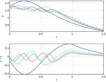
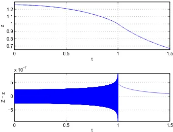
As λ in (14) tends to ∞, the oscillations disappear. (This is demonstrated in Sec. III.) The resulting curve Z(t), which begins at Z(0) = 21/3 and passes through Z(1) = 1, is shown as a dashed line (red in the electronic version) in Fig. 3 (upper panel). Also shown are the first four eigencurve (separatrix) solutions to (14) (blue, cyan, magenta, and green in the electronic version), which have one, two, three, and four maxima. Note that these eigensolutions rapidly approach the limiting dashed curve as the number of oscillations increases. The lower panel in Fig. 3 indicates the difference between the dashed curve and the solid curves plotted in the upper panel.

For large values of λ the convergence to the limiting curve is dramatic. In Fig. 4 we plot the limiting curve Z(t) in the upper panel and the difference between the limiting curve and the n = 500,000 separatrix curve (eigencurve) in the lower panel. Note that the difference is of order 1/n (10−6). On the basis of these numerical calculations we were able to use Richardson extrapolation [8] to calculate the coefficient A accurate to one part in 1010 and we conjectured reliably thatA= 25/6.

The convergence of z(t) (which is rapidly oscillatory when 0≤t≤1) to Z(t) (which is smooth and nonoscillatory) as λ → ∞ strongly resembles the convergence of a Fourier series. Consider, for example, the convergence of the Fourier sine series to the function f(x) = 1 on the interval

0< x < π. The 2N+ 1 partial sum of the Fourier sine series is

S2N+1(x) =

4

π

N

X

n=0

sin[(2n+ 1)x]

0 0.5 1 1.5 0.8

1 1.2 1.4

t

z

0 0.5 1 1.5

−0.2 −0.1 0 0.1

t

Z − z

FIG. 3: Upper panel: Numerical plots of the first four separatrix solutionsz(t) (eigensolutions) to (14) (blue, cyan, magenta, and green in the electronic version). These solutions have one, two, three, and four maxima. Asλincreases, these curves approach the solution to (14) forλ=∞(dashed curve) (red in the electronic version). [Theλ=∞curve is calledZ(t) and satisfies the differential equation (31).] Lower panel: A plot of the differences between the solid curves and the dashed curve.

As can be inferred from Fig. 5, which displays the partial sums for N = 5,20,80, asN increases,

S2N+1(x) approaches 1 (except for values ofxnearx= 0 andx=π) in a highly oscillatory fashion

that strongly resembles the approach ofz(t) to Z(t) in Fig. 4.

III. ASYMPTOTIC SOLUTION OF THE SCALED EQUATION (14)

The objective of the asymptotic analysis in this section is to solve (14) for large λand to verify the result in (9); namely, thatA = 25/6. We begin by converting the differential equation in (14) to the integral equation

[z(t)]2−[z(0)]2+t2/2 +η(t) = O(1/λ) (λ→ ∞), (18) where

η(t) =

Z t

0

ds scos[2λsz(s)]. (19)

To obtain this result we multiply (14) byz(t)+tz0(t), integrate from 0 tot, and use the double-angle formula for the cosine function.

0 0.5 1 1.5 0.7

0.8 0.9 1 1.1 1.2

t

z

0 0.5 1 1.5

−5 0 5

x 10−7

t

Z − z

FIG. 4: Upper panel: Numerical solutionz(t) to (14) corresponding ton= 500,000. No oscillation is visible because the amplitude of oscillation is of order 1/λwhen λis large. Lower panel: Difference between the

n= 500,000 eigencurvez(t) and theλ=∞curveZ(t). Note that the difference is highly oscillatory and is of order 10−6_.

set of moments An,k(t), which are defined as follows:

An,k(t)≡

Z t

0

dscos[nλsz(s)] s

k+1

[z(s)]k. (20) Note thatη(t) =A2,0(t).

For large λthese moments satisfy the linear difference equation

An,k(t) =−1₂An−1,k+1(t)−1₂An+1,k+1(t) (n≥2). (21)

To obtain this equation we multiply the integrand of the integral in (20) by

z(s) +sz0(s)

z(s) −

sz0(s)

z(s) . (22)

(Note that this quantity is merely an elaborate way of writing 1.) We then evaluate the first part of the resulting integral by parts and verify that it is negligible asλ→ ∞ift≤1. In the second part of the integral we replace z0(t) by cos[λtz(t)] and use the trigonometric identity

cos(na) cos(a) = 1₂cos[(n+ 1)a] + 1₂cos[(n−1)a].

By using repeated integration by parts it is easy to show that η(t) in (19) can be expanded as the series

η(t) =

∞

X

p=0

0 0.5

1 1.5

0 p/2

p N=20

N=5

N=80

x

FIG. 5: Convergence of theN = 5, 20, and 80 partial sums in (17) of the Fourier sine series for f(x) = 1. The partial sums of the Fourier series converge to 1 asN → ∞in much the same way thatz(t) converges to Z(t) as λ→ ∞. AsN increases, the frequency of oscillation increases and the amplitude of oscillation approaches zero.

where the coefficients αn,k are determined by a one-dimensional random-walk process in which random walkers move left or right with equal probability but become static when they reachn= 1. The initial condition for the random walk is thatαn,0 = 0 if n6= 2 andα2,0 = 1. The coefficients

αn,k obey the difference equations

2α1,k+α2,k−1= 0, (24)

2α2,k+α3,k−1= 0, (25)

2αn,k+αn−1,k−1+αn+1,k−1 = 0 (n≥3). (26)

(Note thatαn,k= 0 if one of the subscripts is odd and the other is even.) The difference equations (25) and (26) can be solved in closed form, and we obtain the following exact result for n≥2:

αn,k=

(−1)n(n−1)k!

2k_{(k/2 +n/2)!(k/2−n/2 + 1)!}, (27) which holds if nand kare both even or both odd. Finally, we use equation (24) to obtain

α1,2p+1=−1₂α2,2p =−

(2p)!

22p+1_{p!(p+ 1)!} =−

Γ(p+ 1/2)

Thus, the series in (23) for η(t) reduces to the series of integrals

η(t) =− 1

2√π

∞

X

p=0

Γ(p+ 1/2) (p+ 1)!

Z t

0

ds z0(s) s

2p+2

[z(s)]2p+1,

which is valid for t≤1. This series can be summed in closed form:

η(t) =

Z t

0

ds z(s)z0(s)p1−s2_/[z(s)]2₋

Z t

0

ds z(s)z0(s). (29)

There is no explicit reference toλin this expression, so we pass to the limit asλ→ ∞. In this limit the function z(t), which is rapidly oscillatory (see Fig. 4), approaches the function Z(t), which is smooth and not oscillatory. We therefore obtain from (18) an integral equation satisfied Z(t):

[Z(t)]2−[Z(0)]2+1₂t2−

Z t

0

ds Z(s)Z0(s) +

Z t

0

ds Z(s)Z0(s)p1−s2_/[Z(s)]2 _{= 0. (30)}

We differentiate (30) to obtain an elementary differential equation satisfied byZ(t):

Z(t)Z0(t) +t+Z0(t)p[Z(t)]2_−t2 _{= 0. (31)}

This differential equation is easy to solve because it is ofhomogeneoustype; that is, the equation can be rearranged so thatZ(t) is always accompanied by a factor of 1/t. Such an equation can be solved by making the substitution Z(t) =tG(t) to reduce (31) to a separable differential equation forG(t). The general solution forG(t) is

K

t3 = 1 + 3[G(t)] 2

G(t) +p[G(t)]2₋₁

p

[G(t)]2_−1−2G(t)

p

[G(t)]2_{−1 + 2G(t)}, (32)

whereKis an arbitrary constant. The condition thatG(1) = 1 then determines thatK=−4, and we obtain the exact result thatZ(0) = 21/3. We thus conclude thatA= 25/6. This establishes the principal result of this paper.

IV. DISCUSSION AND DESCRIPTION OF FUTURE WORK

A. First Painlev´e transcendent

We believe that the asymptotic approach developed in this paper may be applicable to many nonlinear differential equations having separatrix structure. One possibility is the differential equation for the first Painlev´e transcendent

y00(x) = [y(x)]2+x. (33)

How do solutions to this equation behave asx→ −∞? It is clear that when x becomes large and negative, there can be a dominant asymptotic balance between the positive term [y(x)]2 and the negative term x, which implies that y(x) can have two possible leading asymptotic behaviors:

y(x)∼ ±√−x (x→ −∞). (34)

This asymptotic result is justified because the second derivative of√−x is small compared withx

This problem is interesting because the asymptotic behavior y(x) ∼ −√−x is stable but the asymptotic behaviory(x)∼√−x is unstable. To verify this, we calculate the corrections to these two asymptotic behaviors. It is easy to show that when x is large and negative, the solution to (33) oscillates about and decays slowly towards the curve−√−x[1]:

y(x)∼ −√−x+c(−x)−1/8cos₄

5

√

2(−x)5/4+d

(x→ −∞), (35)

where c and dare two arbitrary constants. The differential equation (33) is second order and, as expected, this asymptotic behavior contains two arbitrary constants.

On the other hand, the correction to the +√−x behavior has an exponential form

y(x)∼√−x+c±(−x)−1/8exp±4₅

√

2(−x)5/4

(x→ −∞). (36)

Thus, if c+ 6= 0, nearby solutions generally veer away from the curve

√

−x as x → −∞. The special solutions that decay exponentially towards the curve√−xform a one-parameter and not a two-parameter class becausec+ = 0. The vanishing of the parameterc+gives rise to an eigenvalue

condition on the choice of initial value of y0(0). For each value ofy(0) there is a set of eigencurves (separatrices). These curves correspond to a discrete set of initial slopesy0(0).

We have performed a numerical study of the solutions to (33) that satisfy the initial conditions

y(0) = 1 and y0(0) = a. There is a discrete set of eigencurves whose initial positive slopes are

a1= 0.231955,a2 = 3.980669,a3 = 6.257998,a4= 8.075911,a5 = 9.654843,a6 = 11.078201,a7 =

12.389217, a8 = 13.613878, a9 = 14.769304, a10 = 15.867511, a11 = 16.917331, a12 = 17.925488.

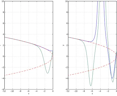
(There is also an infinite discrete set of negative eigenvalues.) The first two of these curves are shown in the left panel and the next two of these curves are shown in the right panel of Fig. 6. Note that the separatrix curves do not just exhibit n maxima as do the dashed curves in Fig. 2. Rather, these curves pass through increasingly many double poles. The curve corresponding to a1

approaches +√−x from above and the curve corresponding to a2 approaches +

√

−x from below. The curves corresponding to a3 and a4 also approach +

√

−x from above and below, but these curves both pass through one double pole. Similarly, the curves corresponding to a5 and a6 pass

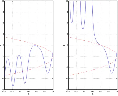
through two double poles, and the curves corresponding to a2n−1 and a2n pass through n double poles. The key feature of these separatrix curves is that after passing throughndouble poles, they approach the curve +√−x exponentially fast asx→ −∞. If the value ofy0(0) lies in between two eigenvalues, the curve either oscillates about and approaches the stable asymptotic curve −√−x

as in the left panel of Fig. 7 or else it lies above the unstable asymptotic curve +√−x and passes through an infinite number of double poles as in the right panel of Fig. 7.

We have used Richardson extrapolation [8] to find the behavior of the numbers an for largen, and we obtain a result very similar in structure to that in (9). Specifically, we find that

an∼Cn3/5 (n→ ∞), (37)

whereC = 4.28373. This number is very close to 17₅21/3. The constant C appears to be universal in that it is seems to be the same for all values of y(0). We are currently trying to apply our analytical asymptotic methods to this problem to find an analytic calculation for the numberC.

B. Conjectural connection with the power-series constant

−12 −10 −8 −6 −4 −2 0 −6

−4 −2 0 2 4 6 8 10

x

y

−12 −10 −8 −6 −4 −2 0

−6 −4 −2 0 2 4 6 8 10

x

y

FIG. 6: Eigencurve solutions to the first Painlev´e trenscendent. The eigencurves pass throughy(0) = 1 and the slopes of the curves at x = 0 are the eigenvaluesan. As x→ −∞, the eigencurves approach +

√ −x

exponentially rapidly. Left panel: first two eigencurves corresponding to the eigenvaluesa1= 0.231955 and

a2= 3.980669. Thea1curve approaches +

√

−xfrom above and thea2curve approaches +

√

−xfrom below. Right panel: The second two eigencurves for the Painlev´e transcendent corresponding to the eigenvalues

a3= 6.257998 anda4= 8.075911. Note that the second pair of eigenvalues passes through one double pole

before approaching the curve +√−x.

but not analytic for|z|< r forr >1. Iff ∈ F, its power-series expansion

f(z) =

∞

X

k=0

akzk

has a radius of convergence of 1. We denote ρn(f) as the largest number r such that the partial sum off(z),

Sn(z) =

n

X

k=0

akzk, (38)

has at least one zero on |z|=r. We define

ρ(f)≡ lim

−12 −10 −8 −6 −4 −2 0 −6

−4 −2 0 2 4 6 8 10

x

y

−12 −10 −8 −6 −4 −2 0

−6 −4 −2 0 2 4 6 8 10

x

y

FIG. 7: Non-eigenvalue solutions to the first Painlev´e transcendent. Ify(0) = 1 buty0(0) is not one of the eigenvaluesan, the curve either oscillates about and approaches the stable asymptotic curve−

√

−xas in the left panel or else it lies above the unstable asymptotic curve +√−xand passes through an infinite number of double poles as in the right panel.

The power series constantP is then defined as

P ≡sup

f∈F

ρ(f). (40)

The precise value for P is not known. However, lower and upper bounds on P have been established. The power series constant was known to lie in the interval 1 ≤ P ≤ 2 until Clunie and Erd¨os [10] sharpened these bounds to √2 ≤ P ≤ 2. Buckholtz [11] further sharpened these bounds to 1.7≤P ≤121/4, which was optimized by Frank [11] to

1.7818≤P ≤1.82. (41) The latter values appear to be the best known values to date. It is astonishing that the value ofA

in (9) agrees with the best known lower bound for the value of P. We do not know whether our value 25/6 coincides exactly with the lower bound. We leave this observation here as coincidence and hope to elaborate on the precise relation in a future paper [12].

functions

fτ(z) =

∞

X

k=0

exp[iπτ(k2+k)]zk (42)

we compute

f_1/4(z) = 1 +iz−iz

2_−z3

1 +z4 (43)

with zeros z1 = 1 and z2/3 =−1/2(1 +i)±

√

2i−4, such that ρ(f1/4) = |z2| ≈1.70002. We can

also compute a value closer to P:

f3/8(z) =

1 +e3iπ4 z+e iπ

4 z2+iz3−iz4−e iπ

4z5−e 3iπ

4 z6−z7

1 +z8 , (44)

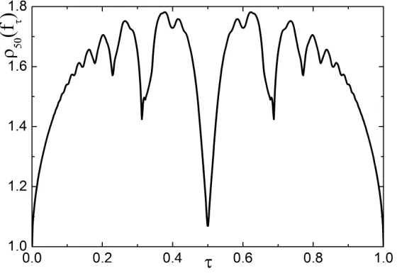
leading toρ f_3/8

≈1.7804. We must terminate the summation and evaluateρn(f) for a sufficiently large value of n. In Fig. 8 we display our numerical results for ρ50(fτ) obtained from the partial sumS50(z). The maximum values are ρ50(f0.3780) =ρ50(f0.8780)≈1.7818, which coincide with the

best known lower bound forP up to the precision of the computation.

FIG. 8: A plot ofρ50(fτ) as a function ofτ. Note that at the optimal value of the parameterτ, the maximum of the curve is very close to the value 1.7818.

C. Final comments

in another asymptotic context, namely, as the lower bound 1.7818 on the power series constantP. We conjecture that the number 25/6 may even be the exact value ofP.

We emphasize that in this paper we have been interested in the limit of large eigenvalues. For linear eigenvalue problems this limit is accessible by using WKB theory. In the case of the nonlinear eigenvalue problem solved in this paper the large-eigenvalue limit is accessible because the problem becomes linear in this limit; indeed, the large-eigenvalue separatrix curve was found by reducing the problem to a linear random walk problem, which can be solved exactly. The strategy of transforming a nonlinear problem to an equivalent linear problem is reminiscent of the Hopf-Cole substitution that reduces the nonlinear Burgers equation to the linear diffusion equation or the inverse-scattering analysis that reduces the nonlinear Korteweg-de Vries equation to a linear integral equation.

There is a plausible argument that the power series constantP is connected with the asymptotic behavior of eigenvalues: On one hand, P is associated with the zero of largest modulus of a polynomial of degree n, which is constructed as the nth partial sum of a Taylor series. On the other hand, a conventional linear eigenvalue problem of the form Hψ = Eψ may be solved by introducing a basis and replacing the operator H by an N ×N matrix HN. Then, to calculate the eigenvalues numerically we find the zeros of the secular polynomial Det(HN −IE). Finding the asymptotic behavior of the high-energy eigenvalues corresponds to finding the behavior of the largest zero of the secular polynomial as N, the degree of the polynomial, tends to infinity.

We believe that the techniques proposed here to find the asymptotic behavior of large eigenvalues may extend to other nonlinear differential equations exhibiting instabilities and separatrix behavior.

Acknowledgments

CMB and JK thank the U.S. Department of Energy for financial support.

[1] C. M. Bender and S. A. Orszag,Advanced Mathematical Methods for Scientists and Engineers(McGraw Hill, New York, 1978), chap. 4.

[2] C. M. Bender, D. W. Hook, P. N. Meisinger, and Q. Wang, Phys. Rev. Lett.104, 061601 (2010). [3] C. M. Bender, D. W. Hook, P. N. Meisinger, and Q. Wang, Ann. Phys. 325, 2332-2362 (2010). [4] J. Gair, N. Yunes, and C. M. Bender, J. Math. Phys.53, 032503 (2012).

[5] See Ref. [1], chap. 10.

[6] For a discussion of hyperasymptotics see M. V. Berry and C. J. Howls, Proc. Roy. Soc. A 430, 653 (1990); M. V. Berry in Asymptotics Beyond All Orders, ed. by H. Segur, S. Tanveer, and H. Levine (Plenum, New York, 1991), pp. 1-14.

[7] See Ref. [1], chap. 11. [8] See Ref. [1], chap. 8.

[9] See Problem 7.7 in W. K. Hayman, Research Problems in Function Theory[Athlone Press (University of London), London, 1967].

[10] J. Clunie and P. Erd¨os, Proc. Roy. Irish Acad.65, 113 (1967). [11] J. D. Buckholtz, Michigan Math. J.15, 481 (1968).