Random compiler for fast Hamiltonian simulation

This is a repository copy of

Random compiler for fast Hamiltonian simulation

.

White Rose Research Online URL for this paper:

http://eprints.whiterose.ac.uk/150026/

Version: Accepted Version

Article:

Campbell, E. (2019) Random compiler for fast Hamiltonian simulation. Physical Review

Letters, 123 (7). ISSN 0031-9007

https://doi.org/10.1103/physrevlett.123.070503

© 2019 American Physical Society. This is an author-produced version of a paper

subsequently published in Physical Review Letters. Uploaded in accordance with the

publisher's self-archiving policy.

[email protected] https://eprints.whiterose.ac.uk/ Reuse

Items deposited in White Rose Research Online are protected by copyright, with all rights reserved unless indicated otherwise. They may be downloaded and/or printed for private study, or other acts as permitted by national copyright laws. The publisher or other rights holders may allow further reproduction and re-use of the full text version. This is indicated by the licence information on the White Rose Research Online record for the item.

Takedown

If you consider content in White Rose Research Online to be in breach of UK law, please notify us by

Earl Campbell1 1

Department of Physics and Astronomy, University of Sheffield, Sheffield, UK (Dated: June 26, 2019)

The dynamics of a quantum system can be simulated using a quantum computer by breaking down the unitary into a quantum circuit of one and two qubit gates. The most established methods are the Trotter-Suzuki decompositions, for which rigorous bounds on the circuit size depend on the number of terms L in the system Hamiltonian and the size of the largest term in the Hamil-tonian Λ. Consequently, Trotter-Suzuki is only practical for sparse HamilHamil-tonians. Trotter-Suzuki is a deterministic compiler but it was recently shown that randomised compiling offers lower over-heads. Here we present and analyse a randomised compiler for Hamiltonian simulation where gate probabilities are proportional to the strength of a corresponding term in the Hamiltonian. This approach requires a circuit size independent of Land Λ, but instead depending on λthe absolute sum of Hamiltonian strengths (theℓ1norm). Therefore, it is especially suited to electronic structure Hamiltonians relevant to quantum chemistry. Considering propane, carbon dioxide and ethane, we observe speed-ups compared to standard Trotter-Suzuki of between 306×and 1591×for physically significant simulation times at precision 10−3_{. Performing phase estimation at chemical accuracy,} we report that the savings are similar.

Quantum computers could be used to mimic the dy-namics of other quantum systems, providing a compu-tational method to understand physical systems beyond the reach of classical supercomputers. A quantum com-putation is broken down into a discrete sequence of ele-mentary one and two qubit gates. To simulate the con-tinuous unitary evolution of the Schr¨odinger equation, an approximation must be made into a finite sequence of discrete gates. The precision of this approximation can be improved by using more gates. The standard approaches are the Trotter and higher order Suzuki de-compositions [1–3]. In addition to simulating dynamics, we are often interested in learning the energy spectra of Hamiltonians. Assuming a good ansatz for the ground state, we can combine quantum simulation with phase estimation to find the energy of the ground state [4] and excited states [5–7]. For a molecule with unknown elec-tronic configuration, this is called the elecelec-tronic struc-ture problem [8, 9] and it is crucially important in chem-istry and material science. However, electronic structure Hamiltonians contain a very large number of terms and unfortunately the gate count of Trotter-Suzkui increases with the number of terms. While the scaling is formally efficient, the required number of gates is impractically large. An alternative to Trotter-Suzkui without this scal-ing problem would therefore have significant applications. A recurrent theme in the literature is that stochas-tic noise can be less harmful than coherent noise [10, 11], which hints that randomisation might be useful for wash-ing out coherent errors in circuit design. Poulinet al[12] showed that randomness is especially useful in simulation of time-dependent Hamiltonians as it allows us to average out rapid Hamiltonian fluctuations. Campbell [13] and Hastings [14] have shown that random compiling can ac-tually help reduce errors below what is feasible with a de-terministic compiler. Since optimisation of Hamiltonian simulation circuits is a special case of compilation, one expects random compilers to be helpful in this setting.

Following this line of reasoning, Childs, Ostrander and Su [15] showed that it is useful to randomly permute the order of terms in Trotter-Suzuki decompositions. How-ever, randomly permuted Trotter-Suzuki decompositions still suffer the same scaling problem that plagues deter-ministic Trotter-Suzuki; that is, the gate count depends on the number of Hamiltonian terms.

Here we propose a simple and elegant approach to Hamiltonian simulation that uses randomisation to cure this scaling problem. Our proposal is similar to Trotter-Suzuki in that we implement a sequence of small rota-tions, without any use of ancillary qubits or complex cir-cuit gadgets. Our key idea is to weight the probability of gates by the corresponding interaction strength in the Hamiltonian. Our simulation scheme can be seen as a Markovian process, which is inherently random but bi-ased in such a way that we stochastically drift toward the correct unitary with high precision. For this rea-son, we call it the quantum stochastic drift protocol, or simply qDRIFT. Unlike any Trotter-Suzuki method, the gate count of qDRIFT is completely independent of the number of terms in the Hamiltonian. Consequently, we find that our approach can speed-up quantum simula-tions of electronic structure Hamiltonians by several or-ders of magnitude within regimes of practical interest. For example of the 60 qubit ethane, we find a speed-up of over a factor 1000 when the approximation error is 0.001 and simulation time is t = 6000 (the same sim-ulation time often used in phase estimation [16]). In quantum chemistry, phase estimation is performed us-ing controlledeitHunitaries and here our techniques can lead to even larger resource savings.

Our analysis is limited in scope in two ways. First, we only compare against other Trotter-Suzuki decompo-sitions. However, there are numerous approaches out-side the Trotter-Suzuki family that make use of ancil-lary qubits and complex gadgets to obtain better asymp-totic performance [17–22], such as the LCU (linear

Protocol Gate count(upper bound) 1st_{order Trotter DET O(L}3_(Λt)2_/ǫ) 2nd order Trotter DET O(L5/2

(Λt)3/2 /ǫ1/2

) (2k)th_{order Trotter DET O(L}2+21k(Λt)1+

1 2k/ǫ1/2k) (2k)thorder Trotter RANDOM O(L2

(Λt)1+₂1 k/ǫ1/2k) qDRIFT (general result) O((λt)2_/ǫ) qDRIFT (whenλ= ΛL) O(L2

(Λt)2 /ǫ) qDRIFT (whenλ= Λ√L) O(L(Λt)2

/ǫ)

TABLE I. Resource scaling for different product formulae (see App. B and C for details and caveats).

binations of unitary) technique. Second, we only com-pare performance of rigorous bounds on gate counts, even though numerical studies of small systems show that far fewer gates are needed than suggested by rig-orous bounds [23–25]. Note that for the special case of local Hamiltonians, tighter analysis is possible because error propagation is localised and obeys Lieb-Robinson bounds [26, 27], but unfortunately electronic structure Hamiltonians are highly nonlocal.

The Hamiltonian simulation problem.- We begin by re-stating the problem more formally. Consider a Hamilto-nian

H =

L X

j=1

hjHj (1)

decomposed into a sum ofHjeach of which is Hermitian

and normalised (such that the largest singular value ofHj

is 1). We can always chooseHj so that the weightinghj

are positive real numbers. Herein we denote λ=P jhj

and remark that this upper bounds the largest singu-lar value of H. The decomposition of the Hamiltonian should be such that for eachHj the unitaryeiτ Hj can be

implemented on our quantum hardware for any τ. Our goal is then to find an approximation of eitH _{into a}

se-quence of eiτ Hj _{gates up-to some desired precision. We}

use the number ofeiτ Hj _{unitaries to quantify the cost of}

the quantum computation, and we aim to minimise the number of such unitaries used. In the simplest Trotter formulae, one divides U =eitH _{into r segments so that} U =Ur

r withUr=eitH/r and uses that Vr=

L Y

j=1

eithjHj/r_{, (2)}

approaches Ur in the larger limit. Furthermore, r

rep-etitions of Vr will approach U in the large r limit, so Vr

r →U. The gate count in this sequence will beN=Lr,

so we would like to know the smallest r that suffices to achieve a desired precisionǫ. Analytic work on this prob-lem (we use the analysis of Refs. [15, 25]) shows that the Trotter error is no more than

ǫ=L

2_Λ2_t2

2r e

ΛtL/r_{, (3)}

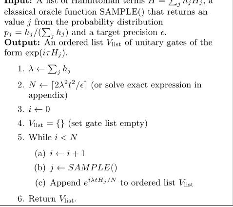
Input: A list of Hamiltonian termsH=P_jhjHj, a

classical oracle function SAMPLE() that returns an valuejfrom the probability distribution

pj=hj/(Pjhj) and a target precisionǫ.

Output: An ordered listVlistof unitary gates of the form exp(iτ Hj).

1. λ←Pjhj

2. N ← ⌈2λ2 t2

/ǫ⌉(or solve exact expression in appendix)

3. i←0

4. Vlist={}(set gate list empty)

5. While i < N

(a) i←i+ 1

(b) j←SAM P LE()

(c) AppendeiλtHj/N _{to ordered listV} list

6. ReturnVlist.

FIG. 1. Pseudocode for the qDRIFT protocol

where Λ := maxjhj is the magnitude of the strongest

term in the Hamiltonian. Solving forr we find approx-imately r _∼ L2_Λ2_t2_{/2ǫ segments are needed, each}

seg-ments containsLunitaries, leading to a total gate count ofN =Lr∼L3_(Λt)2_{/2ǫ. Table 1 compares this against}

other approaches including more sophisticated higher-order Suzuki decompositions. As we increase the higher-order of the decomposition, the scaling approaches O(L2_Λt),

although the constant factors become rapidly worse for higher orders, so that in practice the optimal choice is usually second or fourth order. Childs, Ostrander and Su, showed that randomly permuted Trotter decomposi-tions can further improve the gate count (see Table 1).

Having reviewed the prior art of product formaule, we notice theLdependence never improved below quadratic. Therefore, Trotter decompositions are limited to sim-ulations of quantum systems with sparse interactions, so thatL must scale polynomially with the system size

n. Furthermore, in chemistry problems L =O(n4) and while technically efficient, the resultingO(n8_{) scaling is}

prohibitively large. Next we turn to our protocol that eliminates this dependence.

The qDRIFT protocol.- Our full algorithm is given as pseudocode in Fig. 1. Each unitary in the sequence is se-lected independently from an identical distribution (i.i.d sampling). The strength τj of each unitary is fixed to

a constantτj = τ := tλ/N, which is independent of hj

so, we implement gates of the form eiτ Hj_{. The}

proba-bility of choosing unitaryeiτ Hj _{is weighted by the}

inter-action strength hj, with normalisation of the

distribu-tion entailing thatpj =hj/λ. Therefore, the full circuit

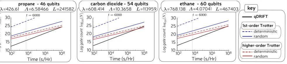
propane - 46 qubits λ=426.61 Λ=6.58466 L=241582

carbon dioxide - 54 qubits λ=608.414 Λ=10.3658 L=113959

ethane - 60 qubits λ=768.138 Λ=4.07041 L=467403

L

og ga

te c

oun

t

log

10

(

N

)

L

og ga

te c

oun

t

log

10

(

N

)

L

og ga

te c

oun

t

log

10

(

N

)

Time (s/Hr) Time (s/Hr)

qDRIFT

deterministic random

1st-order Trotter

higher-order Trotter key

Time (s/Hr) 15

20 25 30

10

102 ₁₀4 ₁₀6 ₁₀8

15 20 25 30

10

102 ₁₀4 ₁₀6 ₁₀8 10₁₀2 ₁₀4 ₁₀6 ₁₀8 15

20 25 30

t= 6000 t= 6000 t= 6000

deterministic random

FIG. 2. The number of gates used to implementU = exp(iHt) for various tand ǫ= 10−3 _{and three different Hamiltonians} (energies in Hartree) corresponding to the electronic structure Hamiltonians of propane (in STO-3G basis), carbon dioxide (in 6-31g basis) and ethane (n 6-31g basis). Since the Hamiltonian contains some very small terms, one can argue that conventional Trotter-Suzuki methods would fare better if they truncate the Hamiltonian by eliminating negligible terms. For this reason, whenever simulating to precisionǫwe also remove from the Hamiltonian the smallest terms with weight summing toǫ. This makes a fairer comparison, though in practice we found it made no significant difference to performance. For the Suzuki decompositions we choose the best from the first four orders, which suffices to find the optimal.

j=_{j1, j2, . . . , jN}that corresponds to unitary

Vj=

N Y

k=1

eiτ Hjk ₍₄₎

which is selected from the product distribution Pj = λ−NQN

k=1hjk. While this quantum process is random,

we build into the probabilities a bias so that with many repetitions the evolution stochastically drifts towards the target unitary. Since each unitary is sampled indepen-dently, the process is entirely Markovian and we can con-sider the evolution resulting from a single random oper-ation. The evolution is mathematically represented by a quantum channel that mixes unitaries as follows

E(ρ) =X

j

pjeiτ Hjρe−iτ Hj (5)

=X

j hj

λe

iτ Hj_ρe−iτ Hj_{. (6)}

Using Taylor series expansions of the exponentials, we have that to leading order inτ,

E(ρ) =ρ+iX

j hjτ

λ (Hjρ−ρHj) +O(τ

2_{). (7)}

We compare this with the channel_UN that is oneNth of

the full dynamics we wish to simulate, so that

UN(ρ) =eitH/Nρe−itH/N (8)

=ρ+i t

N(Hρ−ρH) +O

_t2

N2

,

where we have expanded out to leading order in t/N. Using thatH =P

jhjHj, we have

UN(ρ) =ρ+i

X

j thj

N (Hjρ−ρHj) +O

t2 N2

. (9)

Comparing _E and _UN, we see that the zeroth and first

order terms match wheneverτ =tλ/N. The higher order terms will not typically match and more careful analysis (see App. B) shows that the channelsEandUN differ by

an amount bounded by

δ_≤2λ 2_t2

N2 e 2λt/N

≈2λ

2_t2

N2 , (10)

where the first inequality is rigorous and the approxima-tion on the right is very accurate even for modestN.

Sinceδ is the approximation error on a single random operationE, the error ofN repetitionsEN _{relative to the}

target unitaryU is then

ǫ=N δ.2λ

2_t2

N . (11)

We see the total error decreases as we increaseN. Setting

NtoNqD= 2λ2t2/ǫ(rounding up to nearest integer)

suf-fices to ensure thatN δis less than the required precision

ǫ. The exact value of N is easily calculated, but again the aforementioned approximation is very good.

Asymptotics comparison.- The qDRIFT approach needs approximately 2λ2_t2_{/ǫgates and we include this}

in Table 1 to compare against prior methods. Since it does not explicitly depend on L, there are no sparsity constraints and this is the only known product formu-lae to beat the O(L2_{) barrier. Though one may argue}

thatLdependence is hidden inλ=P

jhj. The bounds

for other Trotter-Suzuki formulae are given in terms of Λ = maxjhj, and these quantities are related byλ≤ΛL.

The worst case for qDRIFT is thereforeλ= ΛL, which occurs for systems like the 1D nearest neighbour Heisen-berg chain [15, 25, 28]. In this regime, qDRIFT is sig-nificantly better than first-order Trotter but the asymp-totics suggest it will be outperformed by higher order Trotter. However, many real world systems have long range interactions that lead to λ ≪ ΛL. For instance, if we hadλ_∼Λ√L then the qDRIFT scaling would be

was the best prior art. While qDRIFT has significantly betterLdependence, it does depend quadratically on Λt

whereas higher-order Trotter approaches linear scaling in Λt. Therefore, for a fixed Hamiltonian, qDRIFT may ex-cel for short times, but there will always be a critical t

value above which it performs worse.

Numerics.- We have generated electronic structure Hamiltonians for propane, carbon-dioxide and ethane by using the openFermion library [29], which naturally sat-isfyλ_≪ΛLand so qDRIFT should perform favourably. We present our results in Fig. 2 using target precision

ǫ= 10−3_{. Observe that qDRIFT offers a significant}

ad-vantage at low t, which is often several orders of mag-nitude better than any prior Trotter-Suzuki decomposi-tion. We remarked in our introduction that t = 6000 has been identified as relevant for phase estimation in quantum chemistry problems [16] and here we see speed-ups of 591_×, 306_×and 1006_×for propane, carbon diox-ide and ethane (respectively). However, since qDRIFT scales worse with tthan higher order Trotter, for longer time simulations our advantage decreases and we even-tually observe a cross-over at times aroundt= 107₋₁₀8

where prior methods perform better. But this cross-over does not occur until the simulation time is so long that 1023

−1025_{gates are required. This is an extremely high}

gate count. Quantum error correction would certainly be needed and it is well known that to implement this many non-Clifford gates would require many billions of physical qubits even with generous hardware assumptions [30–33]. For these molecules, any foreseeable device performing Hamiltonian simulation would significantly benefit from using qDRIFT over standard Trotter-Suzuki.

Phase estimation.- When using phase estimation to find ground state energies, one performs many controlled-exp(iHt) rotations. Estimating energies to precisionδE

— chemical precision means δE ∼ 10−4 — the largest

time used is at leastt_∼π/δE, with slightly longer times

needed to boost the inherent success probability of phase estimation. Note that the Trotter error ǫis not directly connected to δE but instead contributes to the failure

probability. Running phase estimation several times al-lows us to handle modest failure probabilities, so in prac-ticeǫcan be much larger thanδE. Therefore, the relevant ǫ andt regime for phase estimation matches the regime where qDRIFT performs well in simulation tasks. We provide a detailed analysis of phase estimation in App. B, which shows that qDIRIFT offers 2₋3 orders of magni-tude improvement when the failure probability of a single run is 5%.

Diamond norm distance.-An important technicality is that for a random circuit the appropriate measure of er-ror ǫ is the diamond norm distance [34]. If we instead consider a specific instance of a randomly chosen unitary

Vjin Eq. (4), then the error will typically (on average) be much larger thanǫ, with standard statistical arguments

(see e.g. [12]) suggesting it would be closer to √ǫ. It is counter-intuitive that the random circuit error is consid-erably less than the error of any particular unitary, so let us elaborate. If we initialise the quantum computer in state|ψi, then qDRIFT leads to state|Ψji=Vj|ψiwith probabilityPj. If our experimental setup forgets (erases from memory) which unitary was implemented, then it prepares the mixed state

ρ=_EN(_|ψ_ihψ_|) =X j

PjVj|ψihψ|V_j†=

X

j

Pj|ΨjihΨj|. (12) Since this channel isǫ-close in diamond distance to the ideal channelU, it follows thatρisǫ-close in trace norm distance to the target state _U(_|ψ_ihψ_|) = U_|ψ_ihψ_|U†_.

Trace norm distance is the relevant quantity because it ensures that if we perform a measurement, then the prob-abilities of the outcomes (on stateρ) do not differ by more than 2ǫ from the ideal probability given by U|ψi. Pro-vided we estimate expectation values over several runs, each using a new and independent randomly generated unitary, the precision of our estimate will be governed by

ǫrather than the looser√ǫbound obtained without use of the diamond norm.

Discussion.-A common setting is whereHj are taken

as tensor products of Pauli spin operators, then eiτ Hj

can be realised using Clifford gates and a single-qubit PauliZ rotation [35]. When performing quantum error correction, the resource overhead of Clifford gates is neg-ligible [30, 31] whereas the single-qubit PauliZ rotation must be decomposed into a large number of single-qubit

T and Clifford gates. One further advantage of qDRIFT is that it consumes many Pauli rotations of exactly the same angle, allowing the use of adder-circuit catalysis that significantly reduce T-counts [36, 37]. This is es-pecially true when the Pauli rotations then belong to the Clifford hierarchy [38], since one then has the op-tion of directly distilling magic states providing the rota-tion without further compilarota-tion [39–42]. Interestingly, Duclos-Cianci and Poulin [40] give a short discussion of how their magic state distillation protocol could be used in a Hamiltonian simulation scheme using a modified-Trotter decomposition where the gates all have the same

τ value. While they allude to such a Hamiltonian sim-ulation protocol, they do not provide any details or er-ror analysis and nor did they suggest that randomisation would be part of the protocol.

[1] M. Suzuki, Physics Letters A146, 319 (1990).

[2] M. Suzuki, Journal of Mathematical Physics 32, 400 (1991).

[3] D. W. Berry, G. Ahokas, R. Cleve, and B. C. Sanders, Communications in Mathematical Physics 270, 359 (2007).

[4] D. S. Abrams and S. Lloyd, Physical Review Letters83, 5162 (1999).

[5] A. Peruzzo, J. McClean, P. Shadbolt, M.-H. Yung, X.-Q. Zhou, P. J. Love, A. Aspuru-Guzik, and J. L. O’brien, Nature communications5, 4213 (2014).

[6] O. Higgott, D. Wang, and S. Brierley, arXiv preprint arXiv:1805.08138 (2018).

[7] T. O’Brien, B. Tarasinski, and B. Terhal, arXiv preprint arXiv:1809.09697 (2018).

[8] A. Aspuru-Guzik, A. D. Dutoi, P. J. Love, and M. Head-Gordon, Science309, 1704 (2005).

[9] S. McArdle, S. Endo, A. Aspuru-Guzik, S. Benjamin, and X. Yuan, arXiv preprint arXiv:1808.10402 (2018). [10] J. J. Wallman and J. Emerson, Phys. Rev. A94, 052325

(2016).

[11] G. C. Knee and W. J. Munro, Phys. Rev. A91, 052327 (2015).

[12] D. Poulin, A. Qarry, R. Somma, and F. Verstraete, Phys. Rev. Lett. 106, 170501 (2011).

[13] E. Campbell, Physical Review A95, 042306 (2017). [14] M. B. Hastings, Quantum Info. Comput.17, 488 (2017). [15] A. M. Childs, A. Ostrander, and Y. Su, arXiv preprint

arXiv:1805.08385 (2018).

[16] D. Wecker, B. Bauer, B. K. Clark, M. B. Hastings, and M. Troyer, Physical Review A90, 022305 (2014). [17] D. W. Berry and A. M. Childs, arXiv preprint

arXiv:0910.4157 (2009).

[18] D. W. Berry, A. M. Childs, R. Cleve, R. Kothari, and R. D. Somma, in Forum of Mathematics, Sigma, Vol. 5 (Cambridge University Press, 2017).

[19] D. W. Berry, A. M. Childs, R. Cleve, R. Kothari, and R. D. Somma, Physical review letters114, 090502 (2015). [20] D. W. Berry, A. M. Childs, and R. Kothari, in Foun-dations of Computer Science (FOCS), 2015 IEEE 56th Annual Symposium on (IEEE, 2015) pp. 792–809. [21] G. H. Low and I. L. Chuang, arXiv preprint

arXiv:1610.06546 (2016).

[22] R. Babbush, C. Gidney, D. W. Berry, N. Wiebe, J. Mc-Clean, A. Paler, A. Fowler, and H. Neven, arXiv preprint arXiv:1805.03662 (2018).

[23] D. Poulin, M. B. Hastings, D. Wecker, N. Wiebe, A. C. Doherty, and M. Troyer, arXiv preprint arXiv:1406.4920 (2014).

[24] R. Babbush, J. McClean, D. Wecker, A. Aspuru-Guzik, and N. Wiebe, Phys. Rev. A91, 022311 (2015). [25] A. M. Childs, D. Maslov, Y. Nam, N. J. Ross, and Y. Su,

Proceedings of the National Academy of Sciences 115, 9456 (2018).

[26] J. Haah, M. B. Hastings, R. Kothari, and G. H. Low, arXiv preprint arXiv:1801.03922 (2018).

[27] A. M. Childs and Y. Su, arXiv preprint arXiv:1901.00564 (2019).

[28] Y. Nam and D. Maslov, arXiv preprint arXiv:1805.04645 (2018).

[29] J. R. McClean, I. D. Kivlichan, D. S. Steiger, Y. Cao,

E. S. Fried, C. Gidney, T. H¨aner, V. Havl´ıˇcek, Z. Jiang, M. Neeley, et al., arXiv preprint arXiv:1710.07629 (2017).

[30] A. G. Fowler, M. Mariantoni, J. M. Martinis, and A. N. Cleland, Phys. Rev. A86, 032324 (2012).

[31] J. O’Gorman and E. T. Campbell, Physical Review A

95, 032338 (2017).

[32] M. Reiher, N. Wiebe, K. M. Svore, D. Wecker, and M. Troyer, Proceedings of the National Academy of Sci-ences , 201619152 (2017).

[33] E. Campbell, A. Khurana, and A. Montanaro, arXiv preprint arXiv:1810.05582 (2018).

[34] J. Watrous,The theory of quantum information (Cam-bridge University Press, 2018).

[35] N. J. Ross and P. Selinger, Quantum Information and Computation16, 901 (2016).

[36] C. Gidney, arXiv preprint arXiv:1709.06648 (2017). [37] M. Beverland, E. Campbell, M. Howard, and V.

Kliuch-nikov, arXiv preprint arXiv:1904.01124 (2019).

[38] D. Gottesman and I. L. Chuang, Nature402, 390 (1999). [39] A. J. Landahl and C. Cesare, arXiv preprint

arXiv:1302.3240 (2013).

[40] G. Duclos-Cianci and D. Poulin, Phys. Rev. A. 91, 042315 (2015).

[41] E. T. Campbell and J. O’Gorman, Quantum Science and Technology1, 015007 (2016).

[42] E. T. Campbell and M. Howard, Quantum2, 56 (2018). [43] R. Cleve, A. Ekert, C. Macchiavello, and M. Mosca, Proceedings of the Royal Society of London. Series A: Mathematical, Physical and Engineering Sciences 454, 339 (1998).

[44] B. L. Higgins, D. W. Berry, S. D. Bartlett, H. M. Wise-man, and G. J. Pryde, Nature450, 393 (2007). [45] N. M. Tubman, C. Mejuto-Zaera, J. M. Epstein, D. Hait,

D. S. Levine, W. Huggins, Z. Jiang, J. R. McClean, R. Babbush, M. Head-Gordon, et al., arXiv preprint arXiv:1809.05523 (2018).

Appendix A: Error measures

Here we switch to more mathematical notation than used in the main text. We use_||. . ._||to denote the op-erator norm or Schatten-_∞ norm, which is equal to the largest singular value of an operator. We use_||. . ._||1for

the trace norm or Schatten 1-norm, defined as_||Y_||1:=

Tr[√Y†_{Y], which is equal to the sum of the singular}

val-ues of an operator. Throughout, we use the diamond norm distance as a measure of error between two chan-nels. The diamond distance is denoted

d⋄(E,N) =

1

2||E − N ||⋄, (A1)

where_||. . ._||⋄ is the diamond norm

||P||⋄:= supρ;||ρ||1=1||(P ⊗1l)(ρ)||1, (A2)

and will use Pn _{to denote n repeated applications of a}

superoperator. Two key properties of the diamond norm that we employ are:

1. The triangle inequality: _{||A ± B||}⋄ ≤ ||A||⋄+||B||⋄,

2. Sub-multiplicativity: _||AB||⋄ ≤ ||A||⋄||B||⋄ and

consequently_||An

||⋄≤ ||A||n⋄.

From the definition of diamond distance it follows that if we apply the channels_E and _N to quantum state σ, we have that

dtr(E(σ),N(σ)) = 1

2||E(σ)− N(σ)||1≤d⋄(E,N). (A3) The trace norm distance is an important quantity be-cause it bounds the error in expectation values. IfM is an operator, then

|Tr[M_E(σ)]₋Tr[M_N(σ)]_{| ≤}2_||M_||dtr(E(σ),N(σ))

(A4)

≤2_||M_||d⋄(E,N).

IfM is a projection so that this represents a probability, then ||M|| = 1. We see ǫ error in diamond distance ensures that the measurement statistics are correct upto additive error 2ǫ.

Appendix B: Bounding higher order error terms

Next, we make use of the Liouvillian representation of a unitary channel so that

eiHtρe−iHt =etL(ρ) =

∞

X

n=0

tn_Ln_(ρ)

n! , (B1) where

L(ρ) =i(Hρ₋ρH). (B2)

We have that

||L||⋄≤2||H|| ≤2λ. (B3)

Similarly, we can define_Lj that generate unitaries under

HamiltoniansHj so that

L=X

j

hjLj (B4)

and

||Lj||⋄≤2||Hj|| ≤2. (B5)

We will now upperbound the error of the qDRIFT pro-tocol, though remark that a very similar upperbound can be found by employing the Hastings-Campbell mixing

lemma [13, 14]. Each random operator of qDRIFT im-plements a single randomly chosen gate so that

E =X

j

pjeτLj = X

j hj

λe

τLj_{, (B6)}

which expands out to

E = 1l +



 X

j hjτ

λ Lj

 + X j hj λ ∞ X n=2 τn Ln j

n! (B7)

= 1l +τ

λL+

X j hj λ ∞ X n=2 τn Ln j

n! , (B8)

where in the second line we have used Eq. (B4). This is to be compared against

UN =etL/N (B9)

= 1l + t

NL+

∞

X

n=2 tn

Ln

n!Nn

We see the first two terms of_Eand_UN will match

when-everτ=λt/N. Using this value forτ, we have

||UN − E||⋄=

∞ X n=2 tn_Ln n!Nn −

X j hj λ ∞ X n=2 λn_tn

Ln

j n!Nn

_⋄ ≤ ∞ X n=2 tn||Ln

||⋄

n!Nn + X j hj λ ∞ X n=2 λn_tn

||Ln

j||⋄

n!Nn

The first inequality uses the triangle inequality and that all variables are positive real numbers. Next we use sub-multiplicativity combined with Eq. (B3) and Eq. (B5) to conclude that||Ln

||⋄ ≤ ||L||n⋄ ≤(2λ)n and ||Lnj||⋄ ≤

||Lj||n⋄ ≤2n, which leads to

||UN − E||⋄≤

∞ X n=2 1 n! _2λt N n +X j hj λ ∞ X n=2 1 n! _2λt N n = 2 ∞ X n=2 1 n! _2λt N n .

The last equality uses that P

jhj = λ and collects

to-gether the pair of equal summations. Since our definition of diamond distance includes a factor 1/2, we have

d(UN,E)≤

∞ X n=2 1 n! 2λt N n . (B10)

Next, we use the exponential tail bound (see Lemma F.2 of Ref [25]) that states that for all positivexwe have

∞

X

n=2 xn

n! ≤

x2

2 e

x_{, (B11)}

which we use withx= 2λt/N so that

d(UN,E)≤ 2λ 2_t2

N2 e 2λt/N

≈ 2λ

2_t2

The approximation on the right is very accurate in the large N limit. This gives the result stated in the main text. Since the diamond distance is subadditive [34] un-der composition we have that

d⋄(U,EN)≤N d(UN,E) (B13)

=2λ

2_t2

N e 2λt/N

≈2λ

2_t2

N .

Appendix C: Bounding higher order error terms

Here we reproduce for convenience some results on the Trotter and Suzuki decompositions. All these results are taken from Childs, Ostrander and Su [15].

First, we consider the Trotter decomposition, and be-gin by defining

aTROTT:=

(LΛt)2 r2 e

Λt/r_{, (C1)}

bTROTT:=(LΛt) 3

3r3 e Λt/r_.

From this, one can show that deterministic and ran-domised Trotter decompositions have errors

ǫdetTROTT≤ r

2aTROTT, (C2)

ǫrandom TROTT≤

r

2(a

2

TROTT+ 2bTROTT).

One can see that if bTROTT ≪ aTROTT there is a

sig-nificant advantage to the randomised approach. To de-termine gate counts one must solve to find the smallest integer r such that the errors are below some target ǫ. Since the Trotter decomposition hasrsegments and each segment containsL gates, the total gate count isLr.

Next, we consider the 2k-order Suzuki decompositions, starting with the definitions

a2k−SUZUKI:= 2(2·5

k−1_(Λt)L)2k+1

(2k+ 1)!(r2k+1₎ e

2·5k−1_Λt/r , (C3)

b2k−SUZUKI:=

(2_·5k−1_(Λt))2k+1_L2k

(2k−1)!(r2k+1₎ e

2·5k−1_Λt/r .

From this, one can show that deterministic and ran-domised 2k-order Suzuki decompositions have errors bounded by

ǫdet2k−SUZUKI≤ r

2a2k−SUZUKI, (C4)

ǫrandom2k−SUZUKI≤ r

2(a

2

2k−SUZUKI+ 2b2k−SUZUKI).

Again, ifb2k−SUZUKI≪a2k−SUZUKI there is a significant

advantage to the randomised approach. However, in the limitk_{→ ∞}bothb2k−SUZUKI anda2k−SUZUKIapproach

a similar order of magnitude. As such, the advantage of randomised Suzuki decompositions disappears ask in-creases, which was numerically reported by Childs, Os-trander and Su [15]. The other salient point is how the

two terms of ǫrandom

2k−SUZUKI compare in size. In different

limits of Λ, L and ǫ, either the first or second term can dominate. For the Λ andL set by the chemistry prob-lems in the main text and withǫ < 10−2_{, we find that}

the error is dominated by the second term, so a good approximation is given by

ǫrandom2k−SUZUKI/rb2k−SUZUKI, (C5)

≈Bk(Λt)

2k+1_L2k

r2k , (C6)

where in the second line we have also neglected the expo-nential (valid when Λt_≪r) and collected the constants into

Bk =(2·5

k−1₎2k+1

(2k₋1)! . (C7) For chemistry problems we find this approximation to be very close to the exact upper bound. We reiterate that the numerics presented in the main text used the exact expressions, but to gain intuition and study phase estimation these approximations are very useful.

To determine gate counts one must solve to find the smallest integer r such that the errors are below some targetǫ. Using the above approximation one obtains

r= ΛtL

ΛtBk ǫ

21k

, (C8)

where herein we drop the subscripts onǫ. Since the 2k -order Suzuki decompositions haver segments and each segment contains 2_·5k−1_{L gates, the total gate count is}

2·5k−1_{Lr, so we obtain a gate count} Nk = 2·5k−1ΛtL2

ΛtBk ǫ

21k

(C9)

=Ck

L2_(Λt)1+1 2k

ǫ21k

(C10) where Ck is the new constantCk = 2·5k−1B

1/2k k . For

instance we have

N1=

4√2(Λt)3/2_L2

√

ǫ , (C11)

N2= 500

4

√

10(Λt)5/4_L2

3 √4

ǫ , (C12)

N3=

156250√6

2√3

5(Λt)7/6_L2

3√6

ǫ . (C13)

The scaling with Λ, tandǫimproves withk, but the con-stant prefactor becomes large, so in practice one rarely wishes go abovek = 3 and for modestt and ǫ−1 _values

the optimal is often just thek= 1 protocol.

Appendix D: Controlled evolution

..

.

τ Z

2

=

e

=

e

H

Q

=

−

Q

H

Assuming

Q

Q

=

I

..

.

e

_e

iτ Hj

2

Q

Q

†

j

(i)

(ii)

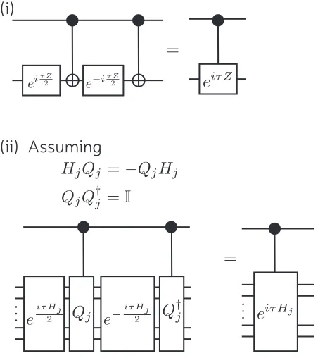
FIG. 3. Implementing controlled rotations used in phase es-timation. (i) a simple circuit for implementing a controlled-exp(iτ Z) gate using two single qubit Z rotations and two control-X gates. (ii) A more general circuit for implementing controlled-exp(iτ Hj), assuming the existence of a suitableQj

operator and the ability to perform control-Qj and

control-Q†_j. Typically, we decompose our Hamiltonian intoHjPauli

operators, in which caseQj and Q†j can be taken to be

sin-gle qubit X or Z operators. Therefore, the decomposition will use two exp(±iτ Hj/2) rotations and two control-X (or

control-Z) gates.

only how to approximate exp(iHt) using qDRIFT. We first observe that controlled-exp(iHt) is equal to exp(i(|1ih1| ⊗H)t). Therefore, we can perform phase estimation by using qDRIFT with the Hamiltonian

H′ =|1ih1| ⊗H (D1)

=|1ih1| ⊗(X

j

hjHj)

=X

j hjHj′

where H′

j = |1ih1| ⊗Hj. Note that ||Hj|| = 1 was

al-ready assumed and implies that_||H′

j||= 1. Furthermore, λ=P

j|hj| andLare unchanged. This allows us to

de-compose the phase estimation circuit into a random prod-uct of exponentials exp(iτ H′

j) = exp(i(|1ih1| ⊗Hj)τ).

Therefore, we see that for a given t and ǫ, controlled evolution needs exactly the same number of exp(iH′

jτ)

rotations as the number of exp(iHjτ) rotations as were

needed for simulation. However, perhaps our hardware can not natively implement exp(iH′

jτ), in which case

there is some additional overhead. However,Hj are

usu-ally Pauli operators, in which case this can be achieved as in Fig. 3 with constant factor overhead.

Appendix E: Phase estimation

Here we analyse and compare using qDRIFT and 2nd

-order random Trotter to implement a simple version of phase estimation in order to perform ground state es-timation. We follow the phase estimation protocol and borrow results from Cleveet. al.[43], though we assume that classical feedforward is used instead of performing the quantum fourier transform (see Fig. 1c of Ref. [44]). There have been many subsequent variants of phase es-timation proposed that could significantly reduce the re-source overhead, but our purpose here is just to demon-strate the utility of qDRIFT rather than give a detailed literature survey of phase estimation techniques.

When using phase estimation to solve the electronic structure problem for Hamiltonian H, we wish to find the energyE0 of the ground state|ψ0i. We do not know

|ψ0ibut can prepare an ansatz state|ψi=P_jcj|ψjithat

has high overlap with the groundstate, sof =_|c0|2≫0.

Phase estimation aims to sample from the energies Ej

with some probability close to_|cj|2. Roughly, the idea is

to perform phase estimation several times and take the lowest reported energy. However, we can only estimate

Ejto finite precision and there is always some probability

of failure. It is useful to defineA:= (H/λ+ 1l)/2, which has eigenvalues in the range 0 to 1. BothH andAshare the same eigenstates, and estimating eigenvalues ofAto additive errorδenables us to estimate the energies to ad-ditive errorδE= 2λδwhere we typically wantδE≤10−4

for chemical accuracy. Given our targetδ we translate this into a number of bits of precisionn = log2(δ)−1,

rounded up. The more bitsn, the more gates are needed in the phase estimation procedure. However, phase esti-mation also has some inbuilt failure probabilitypf that

can be suppressed by using a deeper algorithm. Following Cleveet. al., the depth of the algorithm is determined by

m=n+ log2

1 2pf

+1 2

(E1) = log2(δ−1)−1 + log2

₁

2pf

+1 2

(E2) = log2(δ−1) + log2

₁

pf

+ 1

−2 (E3)

rounded up. The phase estimation protocol uses a se-quence of control-U2j−1

unitaries where U = exp(i2πA) andj = 1, . . . m. We will also write U2j−1

= exp(iAtj)

wheretj = 2jπ.

given earlier, the total failure probability is bounded by

Pf =pf+ 2ǫtot=pf + 2 X

j

ǫj, (E4)

whereǫtot is the total Trotter error summed over all the control unitaries and ǫj is the Trotter error for control-U2j−1

.

1. Failure probabilities

The value ofPf can be quite large without undermin-ing the ground state estimation procedure and we give a rough overview of the statistics involved. As remarked above, we will repeat phase estimation many times. We would need to perform it at least 1/f times to be con-fident that we have sampled the ground state energy. Given a finite failure probability, we need to repeat more times. For instance, we could perform the following pro-cedure: repeat phase estimationM times and record the frequencyν(E) that we observe outcomeE; output the smallest observed E such that ν(E)> Pf + 1/M. The ν(E)> Pf+ 1/M rule will filter out false energies. The expected frequency of measuring the ground state en-ergy satisfies ν(E0)≥f −Pf, provided f >2Pf+ 1/M this approach will (with high probability) ensure that ν(E0)> Pf + 1/M and so the ground state energy will not be filtered out. It is believed that single-determinant Hartree-Fock or known multi-determinant ansatz states usually achievef >1/2 [45] soPf can be quite large (e.g. Pf∼5%−10%) compared toδE.

2. qDRIFT

For each control-U2j−1

unitary, let N(j) denote the number of require gates to achieve the desired ǫj. For qDRIFT, we have

N(j) = 22λ 2 At2j ǫj

= (2 j_π)2 ǫj

, (E5)

= 4 j_π2 ǫj

.

Here the extra factor of 2 comes from Fig. 3. We note that the relevant λis that of the operator A– ignoring the identity component — and soλA= 1/2. We also use tj =π2j. We wish to select ǫj that minimizesPjN(j) subject to the constraint P

jǫj =ǫtot and it is easy to confirm that this is achieved by setting

ǫj=ǫtot 2j

2(2m₋₁₎. (E6)

This leads to

N(j) = 22 j_π2₍₂m

−1)

ǫtot

. (E7)

Summing over allj from 1 tom, we get

N= m X

j=1

N(j) = 4π

2₍₂m₋₁₎2 ǫtot

(E8)

Using Eq. (E1) to substitute in a value form, we find 2m is

2m= 1 4δ

1 pf

+ 1

(E9)

= λ 2δE

1 +pf

pf

, (E10)

Since δE ≤ 10−4 for chemical accuracy, we have that 2m

≫1 and we can take 2m

−1_∼2m_{. Therefore,}

N = π 2_λ2

ǫtotδE2

_{1 +p} f pf

2

(E11)

=π 2_λ2

δ2 E

_{1 +p} f pf√ǫtot

2

Let us define the term in the large brackets as

X:= 1 +pf pf√ǫtot

. (E12)

Using Eq. (E4) to eliminateǫtot in favour ofPf we have

X= 1 +pf pf√ǫtot

=√2 1 +pf pfpPf−pf

, (E13)

We want to minimiseX over all 0_≤pf < Pf and treat-ingPf as a constant. The exact minimal value of X is involved, but assuming smallPf the optimal solution is given bypf = (2/3)Pf. Then the minimal solution sat-isfies X2 _{≤ 27/2P}3

f in the small Pf regime and this is fairly accurate for modest sizePf. Putting this together yields

N ∼27π

2

2 λ2 δ2

EPf3

(E14)

∼133 λ

2

δ2 EPf3

,

where in the last line we have collected the constants and rounded to the first three significant figures.

3. Random Trotter

Next, we follow the same analysis as in the previous section but for second order random Trotter. Then the gate count for control-U2j−1

gate is bounded by

N(j) = 2_·4L2 2Λ 3 At3j ǫj

!12

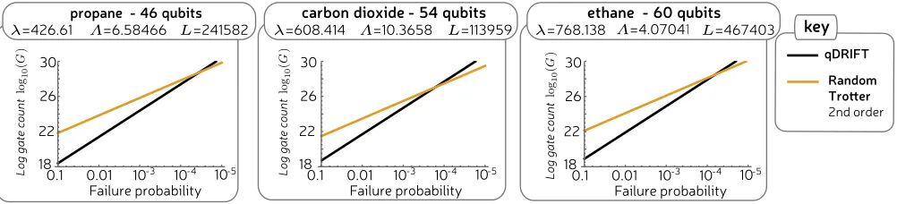
propane - 46 qubits

λ=426.61 Λ=6.58466 L=241582

carbon dioxide - 54 qubits λ=608.414 Λ=10.3658 L=113959

ethane - 60 qubits λ=768.138 Λ=4.07041 L=467403

L og ga te c oun t log 10 ( G ) L og ga te c oun t log 10 ( G ) L og ga te c oun t log 10 ( G ) qDRIFT Random Trotter 2nd order key 22 26 30 18 0.1 Failure probability 0.01 10-3 10-4 10-5

22 26 30 18 0.1 Failure probability 0.01 10-3 10-4 10-5

22 26 30 18 0.1 Failure probability 0.01 10-3 10-4 10-5

FIG. 4. The number of gates used to perform phase estimation withδE= 10−4 as a function of the failure probability.

where the first factor 2 again comes from Fig. 3 and the rest of the expressed is given by Eq. (C11). Here ΛA is for the renormalisedH and so

ΛA= Λ/2λ. (E16)

Withtj=π2j we have

N(j) = 8L2

2π3Λ3A8j ǫj

1 2

. (E17)

The optimal choice ofǫj obeying the relevant constraints is again

ǫj =ǫtot 2 j

2(2m₋₁₎ ∼ǫtot2

j−1−m_{, (E18)}

so that

N(j) = 8L2

₂m+2_π3_Λ3 A4j ǫtot

1 2

(E19)

This leads to

N= m X

j=1

N(j) = 8L2

₂m+1_π3_Λ3 A ǫtot 1 2 m X j=1

2j (E20)

= 8L2

2m+1_π3_Λ3 A ǫtot

1 2

2(2m−1)

∼8L2

_2π3_Λ3 A ǫtot

1 2

232(m+1)

Using Eq. (E9) we find

23m/2_{= (2}m₎3/2₌ λ3/2 23/2_δ3/2

E

_{1 +p} f pf

3/2

. (E21)

and so

232(m+1)= λ

3/2

δE3/2

1 +pf pf

3/2

. (E22)

Substituting this in, we get

N∼8L2

λ3π3Λ3A δ3

E

1 2

1 +pf pfǫ1/3tot

!3/2

. (E23)

We define the contents of the second round pair of brack-ets as where in the last line we define

Y := 1 +pf pfǫ1/3

(E24)

= 21/3 1 +pf pf(Pf−pf)1/3

.

Again, we minimise this, assuming constantPf. We find that for smallPf, the optimal is given by choosingpf = (3/4)Pf. This leads, in the small Pf limit, to Y3/2 ∼ 4.35/P2

f and therefore

N _∼(8_∗4.35)L2

_λ3_π3_Λ3 A δ3 E 1 2 ₁ P2 f . (E25)

Using Eq. (E16) we get

N _∼(8∗4.35)π 3/2

√

8 L

2 Λ3/2 δ_E3/2P2

f

(E26)

= (√8_∗4.35)π3/2_L2 Λ3/2 δ_E3/2P2

f

. (E27)

Evaluating the constant and rounding to nearest integer, we get

N ∼69L 2_Λ3/2

δE3/2Pf2

. (E28)

4. Comparison

Pf = 5% we see speedups of ×1406, ×304 and ×789, respectively. This advantage decreases with smaller Pf and vanishes aroundPf ∼10−4−10−5. However, phase estimation always needed repetition when applied to a state that is not exactly the groundstate (see Sec. E 1). Therefore, as we have already argued, a modest failure probabilityPf = 10%−5% is reasonable.

We finish by repeating our earlier caveats that these plots show known rigorous upper bounds and that actual