Theses Thesis/Dissertation Collections
6-1-2008
A homography-based multiple-camera
person-tracking algorithm
Matthew Robert Turk
Follow this and additional works at:http://scholarworks.rit.edu/theses
This Thesis is brought to you for free and open access by the Thesis/Dissertation Collections at RIT Scholar Works. It has been accepted for inclusion in Theses by an authorized administrator of RIT Scholar Works. For more information, please [email protected].
Recommended Citation
by
Matthew Robert Turk
B.Eng. (Mech.) Royal Military College of Canada,2002
A thesis submitted in partial fulfillment of the requirements for the degree of Master of Science in the Chester F. Carlson Center for Imaging Science
Rochester Institute of Technology
12June2008
Signature of the Author
Accepted by
ROCHESTER, NEW YORK, UNITED STATES OF AMERICA
CERTIFICATE OF APPROVAL
M.S. DEGREE THESIS
The M.S. Degree Thesis of Matthew Robert Turk has been examined and approved by the
thesis committee as satisfactory for the thesis required for the
M.S. degree in Imaging Science
Dr. Eli Saber, Thesis Advisor
Dr. Harvey Rhody
Dr. Sohail Dianat
Date
CHESTER F. CARLSON CENTER FOR IMAGING SCIENCE
Title of Thesis:
A Homography-Based Multiple-Camera Person-Tracking Algorithm
I, Matthew Robert Turk, hereby grant permission to the Wallace Memorial Library of RIT to reproduce my thesis in whole or in part. Any reproduction shall not be for commercial use or profit.
Signature
Date
by
Matthew Robert Turk
Submitted to the
Chester F. Carlson Center for Imaging Science in partial fulfillment of the requirements
for the Master of Science Degree at the Rochester Institute of Technology
Abstract
It is easy to install multiple inexpensive video surveillance cameras around an area. However, multiple-camera tracking is still a developing field. Surveil-lance products that can be produced with multiple video cameras include cam-era cueing, wide-area traffic analysis, tracking in the presence of occlusions, and tracking with in-scene entrances.
All of these products require solving the consistent labelling problem. This means giving the same meta-target tracking label to all projections of a real-world target in the various cameras.
This thesis covers the implementation and testing of a multiple-camera people-tracking algorithm. First, a shape-matching single-camera people-tracking algorithm was partially re-implemented so that it worked on test videos. The outputs of the single-camera trackers are the inputs of the multiple-camera tracker. The al-gorithm finds the feet feature of each target: a pixel corresponding to a point on a ground plane directly below the target. Field of view lines are found and used to create initial meta-target associations. Meta-targets then drop a series of mark-ers as they move, and from these a homography is calculated. The homography-based tracker then refines the list of meta-targets and creates new meta-targets as required.
Testing shows that the algorithm solves the consistent labelling problem and requires few edge events as part of the learning process. The homography-based matcher was shown to completely overcome partial and full target occlusions in one of a pair of cameras.
sored Post-Graduate Training Program.
• Professor Warren Carithers suggested the use of a function used in the Generator program, which was used for testing the algorithm.
• Mr. Sreenath Rao Vantaram supervised the segmentation of all real-world video sequences.
• Finally, Ms. Jacqueline Speir helped me to clarify and expand many of the concepts discussed herein.
1 Introduction 1
1.1 Motivating example . . . 2
1.2 Scope – goals . . . 5
1.3 Scope – limitations . . . 6
1.4 Contributions to field . . . 8
1.4.1 Specific contributions . . . 10
2 Background 11 2.1 Single camera tracking . . . 11
2.2 Multiple camera tracking . . . 14
2.2.1 Disjoint cameras . . . 15
2.2.2 Pure feature matching . . . 16
2.2.3 Calibrated and stereo cameras . . . 17
2.2.4 Un-calibrated overlapping cameras . . . 19
3 Proposed method 21 3.1 Overview . . . 21
3.1.1 Notation . . . 22
3.2 Algorithms . . . 23
3.2.1 Background subtraction . . . 23
3.2.2 Single-camera tracking . . . 27
3.2.3 Field of view line determination . . . 32
3.2.4 Determining feet locations . . . 37
3.2.5 Dropping markers . . . 42
3.2.6 Calculation of a homography . . . 48
3.2.7 Multiple-camera tracking with a homography . . . 53
3.3 Testing and validation . . . 59
3.3.1 Testing the feet feature finder . . . 60
3.3.2 Testing the homography-based tracker . . . 62
3.4 Alternative methods . . . 65
3.4.1 Improving this method . . . 66
3.4.2 The fundamental matrix . . . 69
4 Implementation details 75 4.1 The Generator . . . 76
4.2 Background subtraction . . . 81
4.3 Single-camera tracking . . . 85
4.4 Finding FOV lines . . . 88
4.5 Dropping markers . . . 91
4.6 Calculation of a homography . . . 92
4.7 Homography-based multi-camera tracking . . . 94
4.7.1 Thresholds . . . 94
4.7.2 Speed . . . 95
5 Results and discussion 96 5.1 Feet feature finder . . . 96
5.1.1 Comparing to hand-found points . . . 96
5.1.2 Comparing meta-target creation distances . . . 97
5.2 Homography . . . 103
5.2.1 Markers . . . 103
5.2.2 Numerical tests with truth points . . . 106
5.2.3 Visual tests . . . 108
5.3 Occlusions . . . 117
6 Conclusions and future work 118 6.1 Conclusions . . . 118
6.2 Future work . . . 121
6.2.1 Specific implementation ideas . . . 121
Introduction
Video surveillance is a difficult task. Based on the field of computer
vision, itself only a few decades old, the automatic processing of video
feeds often requires specialized encoding and decoding hardware, fast
digital signal processors, and large amounts of storage media.
The need to process multiple video streams is becoming more
im-portant. Video camera prices continue to drop, with decent “webcams”
available for less than twenty dollars. Installation is similarly inexpensive
and easy. Furthermore, social factors are assisting the spread of
surveil-lance cameras. City police forces, such as those in London and Boston,
and private businesses, such as shopping malls and airports, are using
recent terrorism to justify increasing video surveillance. In most major
cities it is now easy to spot video cameras. Some installations even boast
low-light capabilities using cameras sensitive to near- or thermal-infrared
wavelengths.
Despite the increasing prevalence of multiple camera surveillance
in-stallations, few algorithms extract additional, meaningful multiple-camera
tracking information. Chapter 2 will cover a few of the algorithms that
track moving objects in a single video stream. Solutions to the
single-camera tracking problem are fairly well developed. However,
multiple-camera surveillance systems demand algorithms that can process
multi-ple video streams.
1
.
1
Motivating example
As a motivating example, consider the overhead view of a surveilled area
as seen in Figure 1.1. Cameras A and B are disjoint – they look at
differ-ent areas of the world and do not overlap. However, cameras A and C
partially overlap, as do cameras B and C. An object in either of the darker
overlapping areas will be visible to two cameras simultaneously.
Now examine the output of the three cameras. There are two people in
the world. However, between the three cameras they have been given four
different labels: A-8, B-2, C-4, andC-5. Given these object labels, the most
important piece of information that we could find is which labels refer to
A
C
B C-5
A-8
B-2
C-4
Figure 1.1: Three cameras look at the same general area in this overhead view. Across the three cameras, two targets are given four tracking labels.
Humans are fairly good at solving the consistent labelling problem,
up to a certain point. Human surveillance operators can keep a mental
model of the locations of the cameras in the world, and can often match
features from camera to camera even if different camera modalities are
used (e.g. one RGB camera and one thermal infrared camera).
Addition-ally, humans are much better than computers at matching objects, even
if the objects are observed from widely disparate viewpoints and
conse-quently have different appearances. However, using humans to analyse
multiple video streams does not scale well since a person can only look
at one screen at at time, even though there may be many relevant views
of a scene. If multiple surveillance operators are used, each one
responsi-ble for a particular area, then the system would require the development
of procedures for control, target tracking, target handoff, and possible
[image:11.612.133.498.103.271.2]display/storage Camera 1 input
solo-cam tracking
Camera 2 input
solo-cam tracking
(a) Recording the output of single-camera trackers is common, but does not take advantage of having multiple cameras.
new surveillance capability multi-cam tracking
display/storage
Camera 1 input Camera 2 input
solo-cam tracking solo-cam tracking
(b) Multiple cameras can give ad-ditional information and increase surveillance potential.
Figure 1.2: Algorithms that effectively use multiple cameras can produce extra useful information.
An important task for a surveillance system is being able to track a
target of interest as it moves through a surveilled area. Many cameras
might have the target in view at any given time, but the conscious effort
required of a human to determine this set of cameras is not trivial, even
if only a handful of cameras are used. Additionally, the set of cameras
viewing the target changes constantly as the target moves. If the
con-sistent labelling problem is solved, and the computer knows whether a
target should appear in each camera’s field of view, then the computer
can automatically cue the correct set of cameras that show the target.
Figure1.2illustrates the difference between algorithms that treat
mul-tiple cameras as a group of single cameras, and those that treat the
care that multiple cameras might view the same part of the world. The
second class of algorithms, shown in Figure 1.2(b), take the outputs of
single camera trackers and combine them. New surveillance capabilities
are created. Some examples of the capabilities created by these
multi-camera-aware algorithms are mentioned below.
1
.
2
Scope – goals
This thesis covers the development, implementation, and testing of a
mul-tiple camera surveillance algorithm. The algorithm shall have the
follow-ing characteristics:
1. Independent of camera extrinsic parameters, i.e. location and
ori-entation. The algorithm should smoothly handle widely disparate
views of the world.
2. Independent of camera intrinsic parameters, i.e. focal length, pixel
skew, and location of principal point. Different cameras are
avail-able on the market – the algorithm should be avail-able to handle multiple
focal lengths, differences in resolution, and the like.
3. Independent of camera modality. The algorithm should be able
to handle the output of any single-camera tracker. The algorithm
RGB, near-infrared, thermal infrared, or some other image-forming
technology.
4. Solve the consistent labelling problem. One real-world target should
be linked to one object label in each of the cameras in which that
target is visible.
5. Robust to target occlusions and in-scene entrances. If a target enters
the surveilled area in the middle of a scene, say, through a door,
then the algorithm should correctly solve the consistent labelling
problem. Similarly, if one target splits into two, as when two close
people take different paths, the algorithm should identify and
cor-rectly label the two targets.
6. Simple to set up. No camera calibration should be required.
Train-ing, if needed, should take as little time as possible and should be
done with normal in-scene traffic. Training should be automatic and
should not require operator intervention.
7. Capable of camera cueing. The algorithm should be able to
deter-mine which cameras should be able to see a given target.
1
.
3
Scope – limitations
1. The algorithm shall be used for tracking walking people. Vehicles,
animals, and other classes of moving objects are not included in the
scope of this thesis.
2. Pairs of cameras to be processed will have at least partially
over-lapping fields of view. This requires the operator to make an initial
judgement when installing the hardware and initializing the
algo-rithm: to decide which cameras see the same parts of the world.
3. The cameras shall be static. Once installed, both the intrinsic and
extrinsic parameters of the camera shall be fixed. This means that a
camera can not be mounted on a pan-tilt turret, or if it is, the turret
must not move.
4. The output images of the video cameras will be of a practical size.
The algorithm will not include single-pixel detectors (e.g. infrared
motion detectors, beam-breaking light detectors). This limitation is
necessary to ensure that single-camera tracking is possible without
major changes to the chosen algorithm.
5. Frame rates will be sufficient to allow the single-camera tracking
algorithm to work properly.
6. The cameras shall approximate regular central-projection cameras
view – fisheye lenses – or significant un-corrected distortions will
not be used.
7. Most importantly, the targets shall be walking on a ground plane.
The overlapping area between any two cameras shall not have
sig-nificant deviations from a planar surface. Code to deal with hilly
areas or steps shall not be included in this algorithm.
8. The cameras shall not be located on the ground plane. This prevents
a degenerate condition in the scene geometry, as shall be shown
later.
1
.
4
Contributions to field
As mentioned above, multiple-camera video processing is a relatively
new domain. Algorithms are constantly under development, and there
are many problems yet to solve. If the algorithm developed in this
docu-ment satisfies the goals and limitations described in Sections1.2and 1.3,
then the following scenarios will be made possible:
• Automatic cueing: A target of interest walks into a surveilled area.
The operator marks the target in one camera. As the target moves
throughout the area, the computer, driven by the algorithm,
The target could be marked by a consistently-coloured “halo” or
a bounding box. This lets the operator concentrate on the target’s
actions, rather than on its position in the world relative to every
camera.
• Path analysis: An area is placed under surveillance. Rather than
trying to manually match the paths of people from camera to
cam-era, the algorithm automatically links the paths taken by the people
moving through the area. This enables flow analysis to be carried
out quicker and more effectively.
• Tracking with occlusion recovery. To fool many current tracking
algorithms, move behind an occlusion (e.g. a building support
pil-lar or a tall accomplice), change your speed, and then move out of
the occlusion. Occlusion breaks many current tracking algorithms,
and most others break if the speed change is significant. So long
as the target remains visible in at least one camera, the algorithm
discussed in the forthcoming chapters shall recover from occlusions
and shall re-establish the consistent tracking label.
• In-scene entrances. The algorithm shall be able to create consistent
tracking labels in scenes where people can enter in the middle of a
1
.
4
.
1
Specific contributions
This thesis provides these specific contributions to the field of video
pro-cessing:
• A method to find the feet feature of a target even when the camera
is significantly tilted,
• A method to use target motion to find a plane-induced homography
even when entrances and exits are spatially limited, and
• A method with specific rules describing how to use a plane-induced
homography to create and maintain target associations across
mul-tiple cameras.
The underlying theory is discussed in Chapter3, with implementation
Background
2
.
1
Single camera tracking
Multiple-camera tracking can be done in a variety of ways, but most
methods rely on the single camera tracking problem being previously
solved. Indeed, except for those multiple-camera tracking papers that
aim to simultaneously solve the single- and multiple-camera tracking
problems, most papers include a statement to the effect of ”we assume
that the single-camera tracking problem has been solved.” However, the
present work requires the problem to be actually solved, not justassumed
solved. This is because a working system is to be implemented for this
thesis, not just conceived.
A recent survey of single-camera tracking algorithms is found in [1].
Plainly, a significant amount of thought has been applied to tracking
ob-jects in a single camera’s video stream. When successful, the output is
a series of frames with regions identified by unique identifiers. Two
im-age regions in frames t and t+1 will have the same identifier i if the
algorithm has determined that the regions are the projections of the same
real-world target object. The single-camera tracking problem is how to
determine which regions in frame t+1 to mark with which identifiers.
The survey shall not be replicated here. Instead, we describe a few
char-acteristic approaches to single camera tracking.
One main type of single-camera tracker calculates a feature vector
based on the target, and looks for regions in the next frame that
pro-duce a similar feature vector. The idea of kernel-based object tracking is
introduced in [2]. In this algorithm a feature vector is calculated from
the colour probability density function of an elliptical target region. It
is also possible to use a feature vector based on the target’s texture
in-formation, edge map, or some combination of those and other features,
although those were not tested. In the next frame a number of pdfs are
calculated for candidate regions around the target’s original location. The
candidate regions might have a different scale from the original target, to
take into account looming or shrinking targets. A distance metric is
cal-culated between the original pdf and each of the candidate pdfs. In this
target with the smallest distance to the original target is declared to be the
projection of the same real-world target, and the appropriate identifier is
assigned. It is noted in [2] that other prediction elements can be
incor-porated into the algorithm, such as a Kalman filter to better predict the
target’s new location. Using other prediction elements means that fewer
candidatepdfs must be calculated.
Another type of tracker looks for regions in frame t+1 that have a
similar shape to the target in frame t. A triangular mesh is laid over a
target in [3]. The texture of the object (i.e. its colour appearance) is then
warped based on deformations of the underlying mesh. The warped
tex-ture is then compared to regions in frame t+1 with a metric that
incor-porates both appearance and mesh deformation energy, and the closest
match is called the same object.
Moving farther into shape matching methods, [4] discusses an active
shape model for object tracking. Their algorithm uses a principal
compo-nents analysis to find important points on the boundary of an object in
either grayscale or a multi-colour space. The points are then transformed
using an affine projection into the coordinate space of frame t+1, and
compared with the local textural information. If the transformed points
are close to edges then the model is valid. If points are projected far
from edges then the model is less likely to be correct. Eventually the best
Another method of shape matching, used in this thesis, is introduced
in [5]. The method first uses background subtraction to identify
fore-ground blobs. For basic motion the algorithm assumes that the
projec-tions of each target do not move very far from frame to frame, so they
contain overlapping points. If a target blob in frame t and a candidate
blob in frame t+1 overlap each other but not other blobs, then they are
identified as the same target. If two target blobs merge into one blob in
frame t+1 due to a partial occlusion then the algorithm uses a shape
matching technique introduced in [6]. B-splines are fitted to each
origi-nal target blob in frame t and to groups of regions in frame t+1. The
regions are found using a segmentation algorithm shown in [7]. The
dis-tances between the B-spline control points of the target blob and each set
of candidate regions are compared, then the closest-matching regions are
given the same target identifier.
2
.
2
Multiple camera tracking
When dealing with more than one camera, it is possible that any given
pair of cameras may observe the same area or different areas in the world.
2
.
2
.
1
Disjoint cameras
Algorithms that attempt to associate targets across sets of disjoint
cam-eras use a variety of methods. Some, such as [8], use the entry and exit
times from each camera to learn the structure of the camera network.
From this structure they are able to determine which pairs of cameras
view the same regions of the world, and which are disjoint. The system
can match targets between disjoint cameras so long as people take a
con-sistent amount of time to pass between cameras. A similar approach to
pass target tracks between cameras is used in [9], even if the targets are
invisible some of the time (e.g. between cameras or occluded).
In [10], a set of randomly sampled target point correspondences is
used to create a homography between pairs of cameras. As training data
is accumulated they are able to improve the homography in cases where
the cameras actually overlap, and discard relationships between disjoint
cameras. Their system is thus capable of projecting the location of a
target in one camera to its location in another camera, assuming that
both cameras observe the target.
Three papers by Javed et altake a somewhat more appearance-based
approach to disjoint cameras [11,12,13]. The algorithm finds a brightness
transfer function that projects a target feature vector from one camera
to another. Simultaneously, a Parzen window technique is used to
the various cameras. The projected appearance of a target is then matched
from camera to camera using a Bhattacharyya-distance based metric, and
the results combined with the spatio-temporal matcher to create target
matches.
The present research does not deal with pairs of disjoint cameras.
Rather, we assume that the system has been set to only find matches
between cameras that have overlapping fields of view. If this level of
installation knowledge is unavailable, one of the aforementioned
tech-niques could be used to determine which cameras are disjoint and which
overlap.
2
.
2
.
2
Pure feature matching
Multi-camera feature matching algorithms assume that some features of
a target will remain invariant from camera to camera. A very basic colour
matching method is used to identify projections of the same real-world
target in different cameras [14]. A matching algorithm on the colour
histogram taken along the vertical axis of an object is used in [15].
The method of [16] attempts to reconstruct 3d scene information by
creating associations between posed surface elements (surfels) using
tex-ture matching. This method has not seen much attention because of the
relative complexity of computing scene flow – the3dequivalent of optical
2
.
2
.
3
Calibrated and stereo cameras
If calibration data is available then it is possible to calculate target
fea-tures and use those feafea-tures to match targets between cameras, even if
they are disjoint. Depending on the algorithm, calibration usually means
finding the camera’s internal and external parameters (focal length, field
of view, location, pose, etc.). For instance, [17] uses the height of targets
as a feature that will not change significantly as a target moves from one
camera to another. Both the target’s height and the colours of selected
parts of a target are used to match objects between cameras [18].
The principal axis of a target is the main feature used to match
be-tween cameras [19]. The principal axis is transformed from camera to
camera using a homography found by manually identifying
correspond-ing ground point pairs in both cameras.
In [20], a system is described that is used to track people and vehicles
conducting servicing tasks on aircraft. The system combines
appearance-based methods and the epipolar geometry of calibrated cameras to find
the3dlocations of targets in the scene, and match them accordingly.
Fig-ure 2.1shows the epipolar geometry relation between two views.
Essen-tially, a2dpoint in one camera can be projected to a one-dimensional line
in the other camera, upon which the image of world-point X will lie.
Rather than using epipolar geometry, [21] uses sets of stereo cameras.
Figure2.1:Epipolar geometry: the fundamental matrix Flinks the image points of 3dworld pointXin two cameras byxBFxA=0. eA andeB are the epipoles –
the images of the other camera’s centre.
with appearance-based matching to create maps of likely target locations.
The map for each camera can be transformed until the cameras line up,
at which point full multi-camera tracking can be conducted.
Two papers, [22] and [23], describe methods that require the operator
to specify corresponding ground point pairs in cameras. Those point
pairs lead to a homography between the cameras that can be used to
match targets based on their projected locations in each camera, although
[image:26.612.199.410.137.346.2]2
.
2
.
4
Un-calibrated overlapping cameras
One of the more important recent papers in multi-camera tracking is [24],
by Khan and Shah. This thesis builds on concepts and methods from that
paper. Essentially, the algorithm, discussed at length in Chapter3, records
entry and exit events in one camera, eventually finding the lines created
by projecting the edges of the camera’s field of view onto a ground plane.
Figure 2.2 illustrates this geometry. Once those field of view (fov) lines
are known, target matches can be created between cameras whenever an
object crosses one of those lines. An improvement to the original work is
made in [25] by re-defining when an entry or exit event is detected – this
improvement is discussed in Chapter3.
C
C
A
B
LAB,s
side s
LB,s
Figure2.2: This thesis and [24] find field of view lines on ground planeπ.
There are other approaches that effectively recover a geometric
method, [26] uses a homography-based method to recover from
occlu-sions during which the appearance model can not be updated. The user
effectively specifies the homography. Point intersections are used in [27]
to create a3dmap of the world. Correct point intersections reinforce each
other, leading to higher probability of a match, while incorrect matches
are more scattered around the world, and so lead to a lower probability
Proposed method
3
.
1
Overview
As described in Sections 1.2and 1.3, an algorithm is desired that receives
two video camera feeds from camera A and camera B. The cameras have
at least partially overlapping fields of view. By watching people move
through the scene the algorithm should eventually be able to predict the
location of a person in camera B based solely on their position in camera
A, and vice versa. This thesis will implement three functional objectives:
• Single-camera tracking,
• Learning the relationship between two cameras, and
• Using the relationship to predict target locations.
In Section3.2, various algorithms used in this thesis will be explained.
First, the two parts of single-camera tracking – background subtraction
and object tracking – will be discussed. This will be followed by the
method used to learn the relationship between camera A and camera B,
which consists of two main parts: finding field of view lines and then
accumulating enough corresponding points to calculate a plane-induced
homography. Finally, once that homography is known, the novel
algo-rithm that creates, updates, and refines relationships between targets will
be introduced in Section 3.2.7.
Following the algorithm development, Section3.3 will cover how the
various components of the system will be tested.
3
.
1
.
1
Notation
In general, the following conventions will be used except when we adopt
the notation from specific papers:
• Scalars are represented with lower-case letters. y=3.
• Vectors are represented with bold lower-case letters, and are in
col-umn form. Transposing a vector gives us a list made up of a single
row. xT = [x1x2x3].
• Matrices are represented with upper-case letters. In ˆx = Hx, ˆx and
3
.
2
Algorithms
3
.
2
.
1
Background subtraction
The first step in processing each single-camera input frame is to
deter-mine which parts of the image are background, and hence un-interesting,
and which are foreground. In this work, foreground objects are moving
people. The algorithm first described in [28] and [29], and elaborated
on in [30], describes a system that accomplishes these goals. Although
the system is designed to work on traffic scenes, where the targets (also
known as Moving Visual Objects, ormvos) are cars, the algorithm has the
following desirable attributes:
• The constantly-updated background model can adapt to changing
lighting conditions, objects becoming part of the scene background
(e.g. parking cars), and formerly-background objects leaving the
scene (e.g. departing cars);
• Shadow-suppression; and
• Parameters to tune for various object speeds and sizes.
The general flow of the algorithm can be seen in Figure3.1.
The background model is made up of a number of the previous frames,
held in a FIFO queue. A number of methods can be used to initialize the
Identify shadows
Identify MVOs and ghosts
Identify MVO shadows
Update background model Read in frame
MVO map
Figure3.1: The background subtraction algorithm from [30].
slot in the queue, although if the frame has foreground elements then the
MVO map will be incorrect at the start of processing. Alternatively, the
algorithm can be set to run in a training mode, reading in, say,100frames.
The median of those frames can then be calculated and the result used to
fill the background model queue. The number of frames used to generate
this model is a trade-off between the amount of memory available and
the amount of traffic in any particular pixel. The method to calculate the
background image from the buffer is described below.
In the main loop, there is a background imageB. Any particular pixel,
p, in the background has a hueBH(p), saturationBS(p), and valueBV(p),
which are easily calculated from the pixel’s red, green, and blue values.
An image, I, is read from the incoming video stream. Pixel p in the
[image:32.612.206.400.138.321.2]Once an image has been read, the first step is to identify shadow
pixels. Pixel p in the shadow map, SM, is classified as shadow if:
SM(p) = 1 if
α ≤ IV(p)
BV(p)
≤β
| IS(p)−BS(p)|≤ τS
min(| IH(p)−BH(p) |, 2π− | IH(p)−BH(p)|) ≤τH
0 otherwise
(3.1)
The first condition lets pixels be shadow if they have a value ratio
between two thresholds. In [29] a preliminary sensitivity analysis was
carried out, with values ofα ∈ [0.3, 0.5] and β∈ [0.5, 0.9].
The next two conditions essentially require that the image pixel have
the same colour as the background. Thresholds τS and τH are set by the
user. In the analysis mentioned above, τS ∈ [0.1, 0.9]and τH ∈ [0, 0.1].
Once the shadow map has been created, mvos are identified. First,
every image pixel’s distance from the background is calculated. The
dis-tance measure used is the largest absolute difference from the background
of each of the pixel’s hue, saturation, and value.
Pixels withDB(p)lower than a thresholdTLare not given further
con-sideration as foreground. A morphological opening is performed on the
blobs of pixels with DB(p) > TL. Following the opening, any pixels that
were previously found to be shadows are turned off, not to be considered
as potential foreground pixels. Next, each remaining blob is checked for
three conditions. If the blob satisfies all three conditions, then its pixels
are labelled as part of anmvo.
• The blob has an area larger than thresholdTarea.
• The blob contains at least one pixel with DB(p) > TH. Note that
TH >TL.
• The blob’s average optical flow must be above threshold TAOF.
Objects that do not meet all three criteria are called ghosts. No
guid-ance is given in [30] on how to select the thresholdsTH,TL, Tarea, or TAOF.
Specific implementation details used in this thesis are discussed in the
Chapter 4.
At this point, the MVO map has been created, and can be passed to
the single-camera tracking algorithm. However, the background model
must still be updated for the next frame. To do this, the shadow map is
partitioned into foreground shadows and ghost shadows. Shadow pixel
foreground shadows. Ghost shadows are pixels in shadow blobs that do
not touch an MVO.
There are now five possible classifications for any given pixel:
fore-groundmvo, foreground shadow, background, ghost, and ghost shadow.
The background model update proceeds as follows:
1. Pixels in the current frame that have been marked as foreground or
foreground shadow are replaced with the pixels from the current
background image.
2. The modified current frame is pushed onto the background FIFO
queue. The oldest image, at the end of the queue, is discarded.
3. n images are selected from the buffer, equally spread by m
inter-vening frames. For instance, every fifth image might be selected
(m = 5), with eight images in total (n = 8). The queue is sized
n×m.
4. The median of the selected is calculated. The result is the updated
background image for the next incoming frame.
3
.
2
.
2
Single-camera tracking
In order to associate targets using multiple cameras, we first need to track
is the output of the background subtraction algorithm, namely, a series
of blob masks that is non-zero on foreground pixels, and zero elsewhere.
The output of the single-camera tracker can be represented many ways.
In the present work the output is a frame-sized array, with each pixel’s
value an integer corresponding to a blob label. As targets move around
the scene the shape and position of their corresponding blob changes with
the output of the background subtraction algorithm. After single-camera
tracking, the value of the pixels in each target’s blob should be constant.
We add the additional requirement that target labels should be
histor-ically unique. This means that once a target disappears from the scene,
whether by leaving the field of view of the camera or by being
fully-occluded, its tracking label is not used again.
Depending on the machine architecture, the language used, and the
expected run times it is possible that the target label variable may
even-tually overflow. If this event is expected to occur inside the temporal
window where the oldest target and the newest target are active in some
part of the surveilled area, then there might be a problem. Since the
scenes used in this research were fairly short and had low traffic rates,
we did not encounter this problem when using 16-bit unsigned integer
target labels (65,535possible labels).
The single-camera tracking algorithm used in this thesis can be found
track-ing blobs from frame to frame. In more complex motion cases, such
as partial occlusion, merging, and splitting, the algorithm uses a
shape-matching technique developed in [6]. The following is a brief overview
of the single-camera tracking algorithm; for more detail the reader is
en-couraged to examine the original papers.
Overlap tracking
In an un-crowded scene, targets move around without being occluded by
other moving targets. In this case tracking is a fairly simple process if
one key assumption is made: slow motion. This means that targets are
required to be imaged in such a position that they partially overlap their
previous location. For most surveillance applications with
reasonably-sized targets and normal video frame rates, this is a reasonable
assump-tion.
Given a map of foreground pixels identified by the background
sub-traction algorithm for framet, and the output of the single-camera tracker
from the previous cycle (framet−1), we perform the following tests:
• Does each blob in frame t overlap any previously-identified targets
in frame t−1? If so, how many?
• How many blobs in framet overlap each target from framet−1?
It is given a new target label, and the new target counter is incremented.
If the answer to the both questions is exactly one then the slow
mo-tion assumpmo-tion means that the blob is the same target as the one that it
overlaps. Thus, the blob in frame t inherits the target label from frame
t−1, and for that blob, tracking is complete.
Complex motion – splitting
If two or more unconnected blobs in the current frame t overlap one
contiguous target in framet−1, then this indicates a splitting event. This
could happen when two people who originally walked side-by-side take
different paths.
In this case, [5] says that the largest blob in frame tshould inherit the
tracking label from frame t−1, and the smaller blob(s) should receive a
new, unique tracking label(s).
Complex motion – merging
If a contiguous blob in frame toverlaps more than one previously
identi-fied target region then we must determine which pixels in the blob belong
to each of the old targets. This situation occurs whenever two targets walk
towards each other – there is a period of time when one target partially
occludes the other. Matching is done using the shape matching technique
1. The current frame is segmented into regions based on colour and
texture information using the algorithm found in [7].
2. B-splines are fitted around various segments, starting with the
seg-ment that has the largest area. The splines are fitted according to
algorithms found in [31].
3. The B-spline control points of the targets in frame t−1 are
com-pared to the control points of shapes made up of the frame t image
segments using a metric based on the Hausdorff distance. The
met-ric is invariant to affine transformations [6].
4. The segments that make up the best match for each of the previous
target shapes inherit the old tracking labels.
Note that if one target fully occludes the other then the occluded
tar-get’s tracking label is deprecated and is not used again. When the
oc-cluded target emerges from full occlusion back into partial occlusion the
tracker essentially believes that the occluding target is growing.
Eventu-ally the targets split into two non-contiguous blobs, and are treated as
a described in the splitting section, above. Thus, when a target passes
through full occlusion, it will emerge with a new target label not related
3
.
2
.
3
Field of view line determination
Finding the relationship between the objects in camera A and objects in
camera B can be broken into two parts. The first part consists of finding
Field of View (fov) lines and creating target associations using a modified
implementation of [24]. That algorithm shall be described in this
subsec-tion. The second part consists of using the meta-target information to
create a list of corresponding points (Section 3.2.5), and then using those
points to find the plane-induced homography (Section 3.2.6).
As discussed in the previous chapter, the aim of [24] is similar to the
aim of this work. In short, we want to find the relationship between
mov-ing people as seen by cameras A and B. Whereas this thesis’s approach
wishes to find the correspondence between targets at any point in the
frame, the fov approach is designed to create meta-targets based on a
single correspondence event between tracks of moving objects. This
sin-gle correspondence event occurs when the target passes into or out of
the field of view of camera B. That instant is known as an “fov event”.
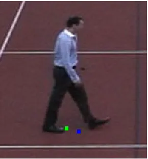
In [25] anfovevent is slightly redefined to be the time at which an object
has completely entered a scene, and is not touching any frame edge. fov
events are also triggered at the instant when an in-scene target begins to
touch a frame edge. In the code implemented for this thesis we use the
modified definition of an fovevent. Figure 3.2 shows a target just as it is
In the following paragraphs we use notation from [24].
Figure3.2: In camera B a target is almost completely in the field of view. When no part of the target mask touches the frame’s edge then an fov event is
trig-gered.
Once anfovevent has been triggered by objectk as seen in camera B,
OkB, the fov constraint allows us to choose the best matching object OA i
from the set of all moving objects in camera A,OA. We quote from [24]:
If a new view of an object is seen in [camera B] such that it has
entered the image along side s, then the corresponding view
of the same object will be visible on the line LBA,s in [camera A]
The line LBA,s is the field of view line of side sof camera B, as seen by
camera A. This is illustrated in Figure3.3.
The algorithm essentially has two steps: learn thefovlines of camera
C
C
A
B
LAB,s
side s
LB,s
Figure3.3: The top side of camera B projects to a line on ground planeπ, shown as LπB,s. That line is then imaged by camera A asL
B,s A .
steps into camera B. Automatic recovery of the fov lines is done by
fol-lowing these steps:
1. Whenever a target enters or leaves camera B on side s, trigger an
fov event.
2. When anfov event has been triggered, record the feet feature
loca-tions of all targets in camera A. Note that each side of camera B will
have its own map of accumulated feet locations.
3. After a minimum number of fov events have been recorded,
per-form a Hough transper-form on the map of feet points. The result is the
fov line in camera A,LB,s A .
Thereafter, whenever a target crosses sides of camera B, triggering an
to LBA,s. To find the target with the feet closest to thefov line, we can use
the homogeneous representation ofLBA,s: l= [a b c]T withax+by+c =0,
scaled such thata2+b2 =1. xand ycan be taken as positions on the row
and column axes of camera A. If the homogeneous representation of the
target’s feet point is used, x = [x y 1]T, then the perpendicular distance
from the line to the feet point is given by the dot product d=lTx.
The initial association of targets as they crossfovlines essentially
cre-ates a point correspondence between the two feet feature locations. Khan
and Shah say that they can use those point correspondences to find a
homography between the two cameras [24]. Once the homography is
known, they can use it to predict target locations, thereby creating
tar-get associations for tartar-gets that are not close to a fov line. Although a
projective transformation was noted to be the general solution, [24] noted
that an affine transform was sufficient for their purposes. No details are
given on how to implement this homography-based matching system.
If only one side is used by targets to enter and exit the frame then the
homography will be degenerate, and the matching system will not work.
The method described in [25] also attempts to find a homography
us-ing point correspondences. However, instead of relyus-ing on target-created
point correspondences, they use the four points created by intersecting
fov lines. This method requires that all four fov lines be known. If one
ho-mography is not computable with this method.
The method of [25] also introduces a potential source of error: because
fov events are triggered when the target is fully inside the frame, the
camera B fov lines are displaced towards the centre of the frame. Yet
the corner points, used for the calculation of the homography, are left at
the corners of the frame. Because the homography only uses four points,
it is exact (i.e. it is not a least-squares error-minimizing solution with
many input points), so it will certainly contain errors. The exact nature
of the error will depend on the angle of the cameras, the average height
of segmented targets, and whichfov lines are inaccurate.
In relying solely on thefovline point correspondences, [24] effectively
makes the following assumptions:
1. At the moment they cross an fov line, all targets are properly
seg-mented in both viewpoints.
2. The location of the feet feature is correctly determined for all targets.
3. A homography based on points nearfovlines will predict feet
loca-tions for targets in the middle of the frame with sufficient accuracy
to associate targets from camera to camera.
Ideally, these restrictive assumptions will be valid. However, if the
seg-mentation of targets is incorrect in either camera, either through addition
(i.e. mvopixels not included in the target’s mask), then the feet locations
will be incorrectly identified. This will have many knock-on effects: the
fovlines will be skewed; a target may be incorrectly judged as being
clos-est to the fov line; the list of corresponding points will be incorrect; and
thus the homography used for matching might contain significant errors.
We overcome these potential sources of error using methods
intro-duced below in Sections 3.2.5 and 3.2.7. First, we discuss two ancillary
algorithms: how to find the feet feature, and how to calculate a
homog-raphy given a list of corresponding points.
3
.
2
.
4
Determining feet locations
Finding the feet of a moving object is essentially a feature detection
prob-lem. In the present case, the input to the feet locator function will be a
mask of a moving object – a standing or walking person. The challenge is
to find a single point that represents the “feet” of that person. In general,
a person will have two feet touching or nearly touching the ground. The
single point then can be thought of as representing the location of the
person’s centre of gravity, projected onto the ground plane.
As mentioned above, the requirement for a single point stems from
our desire to project that point into another camera’s coordinate system.
The projection of a person’s centre of gravity should be onto the same
(a) The feet are said to be at the centre of the bottom edge of the bounding box.
(b) If a target is tilted rela-tive to the camera, then the method will fail to correctly identify the feet location.
Figure3.4: The method of finding the feet feature location from [24].
In [24], Khan and Shah drew a vertical rectangular bounding box
around a moving object. The target’s feet were then deemed to be
po-sitioned at the centre of the bottom edge of the bounding box. This can
be seen in Figure 3.4(a). This method is widely used in the computer
vision community.
The bounding-box method of finding feet described in [24] has a
[image:46.612.160.445.123.449.2]their height axis aligned with the vertical axis of the camera. If the camera
is tilted relative to the person, which could occur if the camera is installed
on a tilted platform or if the person has a consistent tilt in their gait, then
the bounding box will enclose a large amount of non-target area. As a
result, the bottom centre of the bounding box will not necessarily be close
to the actual feet of the target. Figure3.4(b) shows this error mode.
The second failure mode of the bounding-box feet-finding method is
that the feet will always be outside of the convex hull formed by the target
mask. This means that the feet will always appear below the actual feet
location. When considered in three dimensions for targets on a ground
plane, this means that the feet will always be marked closer to the camera
than they should be. Given a wide disparity in camera views, the
pro-jected locations of the feet in each view will not be at the same point –
the feet will be marked somewhere between the best feet location and the
cameras’ locations.
Instead of relying on the camera and the target’s height axis to be
aligned, if the target is rotated to a vertical position then the problem of
tilted targets is eliminated. One of many methods to find the rotation
angle is to perform a principle components analysis (pca) on the target
mask. On a two-dimensional mask, the output of the pca can be
inter-preted as a rotation that overlays the direction of maximum variability
appear to be much taller than they are wide, so the direction of maximum
variability will be the height axis.
Once the pca has rotated the object to eliminate the effect of a tilted
target, the actual position of the feet needs to be found. Instead of simply
using the centre of the bottom of the rotated bounding box, which may
lead to an inaccurate feature location as described above, the following
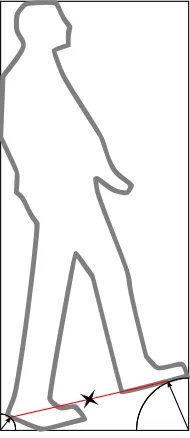
method can be employed:
1. Trace the outline of the target mask.
2. For each point on the outline of the mask, find the distance to the
two bottom corners of the bounding box.
3. Find the point with the smallest distance to each of the two corners.
4. The feet are located halfway between those two points.
The method is illustrated in Figure3.5.
Height determination
Section 3.2.5, below, requires the measurement of the height of a target.
This is a solved problem for calibrated cameras: [32] showed a method
to find the actual in-world height of an target. However, this thesis does
not use calibrated cameras. Luckily, the algorithm does not need the
Figure 3.5: After using pca to align the height axis with the bounding box,
the two points on the target’s outline closest to the bounding box’s corners are averaged. The result is the location of the feet feature.
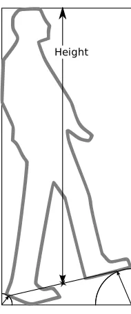
The method to determine the height begins similarly to that described
when finding the feet above. Again, since a target may be rotated with
respect to the camera’s vertical axis, we can not simply take the height of
the bounding box as the height of the object. Rather, thepcaalgorithm is
applied to the pixels in the target mask, and the target is rotated upright.
Now the vertical axis is parallel with the target’s height axis. At this stage
there are two options, simply take the height of the bounding box as the
height of the target, or find the feet feature and take the vertical distance
from that point to the top of the bounding box as the height. The latter
[image:49.612.258.353.138.357.2]Height
Figure 3.6: The height of a target is the vertical distance between the feet and the top of the correctly-oriented bounding box.
In contrast to the feet, the head of a target does not split into two
elements, so the top of the bounding box is nearly always at the correct
location on the target’s head. Furthermore, the shoulders and arms are
often closer to the bounding box corners than the closest head pixel. This
justifies not using the same feet-finding method on the head, and instead
simply using the top of the bounding box.
3
.
2
.
5
Dropping markers
In Section 3.2.3 we noted that [24] used only corresponding point pairs
[image:50.612.257.352.133.360.2]homog-raphy Hπ. These points naturally line the edges of the frame of camera B.
However, since only one point is created for each target (unless the target
surfs thefov line), the correspondence points will be sparse. Depending
on where targets enter and exit the frame, there may be many collinear
correspondences on one fov line and only a few on the other lines. If
only one edge serves as an entry and exit point, then all the accumulated
feet locations will be collinear, and the homography will be degenerate
for our purposes.
Another method was introduced in [25]: using exactly the four points
that are formed by intersecting the fovlines and the corners of the frame
of camera B. This method has a large potential pitfall: if one or more fov
lines are unknown, then the method can not work. It is trivial to find a
situation where an fovline can not be found – anytime camera B has one
edge above the vanishing line of the plane formed by the targets’ heads
(i.e. slightly above the horizon), no targets will trigger edge events on that
edge. Therefore, that fov line will never be found, and the homography
will never be computable.
An improved method to generate the homography is desired. Ideally,
the method will have the following attributes:
• Many corresponding points,
• Able to create corresponding points even if all targets enter and
leave the scene through the same edge.
In [33], H¨ansel and Gretel drop a trail of bread crumbs behind them
as they travel through the woods. We adapt this idea of a trail of bread
crumbs to the present algorithm. In this case, the bread crumbs, also
called markers, are located at the feet feature of each target, which is
assume to be a point on the ground plane π. This can be seen in Figure
3.7.
Figure 3.7: As targets move through the scene, they leave trails of markers be-hind them. These markers are pairs of point correspondences.
After a meta-target is created by associating a target from camera A
with a target from camera B, at an fov event or using the
homography-based method described in Section 3.2.7, the marker-dropping algorithm
begins. The logical flow through the algorithm is shown in Figure 3.8.
marker. If the tests are passed then a marker is dropped, thereby creating
a corresponding point pair.
Wait 1 frame
Wait N frames Add marker to list
Are both MVOs
completely inside frame?
Find height of both MVOs
Are both heights close to historical median?
Is at least one feet location significantly different from last marker? Yes No Yes Yes No No
Figure 3.8: The flow of the corresponding-point generation algorithm. After creation, this algorithm is run on every meta-target.
The first test simply detects whether both target masks are completely
inside their respective frames. If one target is even partially out of the
frame then it is impossible to say with certainty where the feet feature is
located. Therefore, it is a bad idea to create a corresponding point pair.
The second test is of the height of the target. This test is designed
to prevent a marker from being dropped if in that particular frame the
target is grossly mis-segmented or partially-occluded. The method used
to determine the target height was outlined in Section 3.2.4. The height
of an object is measured in pixels, and compared to the median of the
heights in the past few frames. If the height is similar, then we pass on
meta-target until the next frame. This test should work because the height
of a target should not change radically over the course of a few frames.
So long as the threshold is well-chosen, this test should only throw away
badly-segmented or partially-occluded targets.
The third test is to determine whether there has been significant
mo-tion in the past few frames. The distances of the meta-target’s feet features
from the last marker location are calculated. One of the following three
cases must be true:
• Both feet features are close to the previous marker. This means that
the target has not moved much since dropping the last marker.
Cre-ating a new marker will essentially duplicate the previous marker,
so it is not useful. No marker should be dropped in this case.
• Exactly one of the targets has moved away from the previous marker.
This could have two explanations.
The first possibility is that the target has moved towards or away
from one camera centre. In that camera the target will appear in
nearly the same location. However, in the other camera the target
might be seen to move across-frame. This motion is important in
the creation of the homography, so the marker should be dropped.
The second explanation is that the target was segmented as
last marker was dropped, but it still passed the height test. In this
case adding the marker to the list will will likely increase the
accu-racy of the homography. This is because on average we expect the
feet feature to be correctly identified, so any incorrect feet will be
drowned out in the least-squares nature of thedlt algorithm.
• Both targets have moved away from the previous marker. This
prob-ably indicates real target motion. In this case a marker should be
dropped.
One of the requirements stated in Section1.3 was that neither camera
can be on the ground plane. If the camera is in the ground plane then all
of the markers in that camera will appear on a line – the line formed by
the intersection of the camera’s focal plane and the ground plane. This
geometry forces the markers to be collinear, which leads to a degenerate
homography.
The end result is a list of corresponding points. If plotted on the
frame, the points will follow show the historical tracks of the meta-targets.
Depending on meta-target movement – how people walk through the
environment – the points may initially be roughly collinear. A
homog-raphy calculated based on corresponding points when one set of points
is collinear will be degenerate. Therefore, before calculating the
3
.
2
.
6
Calculation of a homography
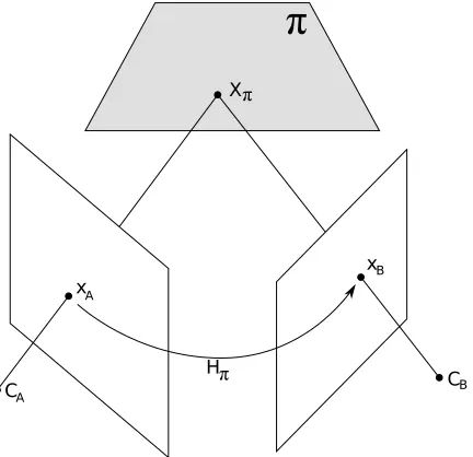
Given a point that lies on a world planeπ, X= [X1 X2 X3 1]T we wish to
find a predictive relation between the images of X in two cameras. That
is, given image points x= [x1 x2 1]T and x0 = [x01 x021]T, we wish to find
Hπ such that
x0 = Hπx (3.3)
Hπ is said to be the homography induced by the world plane π. It
can be thought of as two projectivities chained together: one that takes
a two-dimensional point from the image plane of the first camera, x, to
a two-dimensional point on plane π, and a second that takes a point
from plane π to a point on the second camera’s focal plane, x0. (Note
that a point that lies on a plane in the three dimensional world only has
two degrees of freedom – those that are required to move on the two
dimensional plane.) The geometry of such a scene can be seen in Figure
3.9.
Calculation of Hπ is a fairly simple using the Direct Linear
Transfor-mation (dlt) algorithm. We follow the notation used in [34]. First, given
X
CA CB
x
x
A
B
H
Figure 3.9: A world planeπ induces a projective homography between the two image planes. xB = HπxA. After [34] Fig. 13.1
we can take the cross product of Equation3.3:
x0i×Hπxi =x
0 i×x
0
i =0 (3.4)
If expanded, the cross product can be written explicitly as a matrix
multiplication with the elements:
0T −w0ixTi y0ixTi
wi0xTi 0T −x0ixTi
−y0ixiT x0ixTi 0T
h1 h2 h3
= Aih=0 (3.5)
[image:57.612.200.416.137.346.2]lexico-graphic ordering:
H =hh1 h2 h3i (3.6)
In Equation 3.5, it can be seen that the third row is actually a linear
sum of the first two rows. Therefore, there are only two linearly
indepen-dent rows in Ai. This makes intuitive sense. Each point correspondence
provides two constraints on the homography. The third element in each
homogeneous point, wi and w0i, are simply scale factors that do not
con-strain H.
Therefore, if we only write the first two rows of Ai for each of the
n ≥ 4 point correspondences, then we can stack each Ai into a 2n×9
matrix A. Assuming that we have some measurement noise in our pixel
locations, then the solution to Ah = 0 will not be exact. We therefore
attempt to minimize kAhk. As shown in [34], finding the solution that
minimizes kAhk is equivalent to minimizingkAhk/khk.
The solution is the unit singular vector corresponding to the smallest
singular value of A. By taking the Singular Value Decomposition (svd)
of A, such that A = UDVT, h is the column in V corresponding to the
smallest singular value in D. H is obtained by simply rearranging the
Data normalization
In [35], Hartley noted that many users of the 8-point algorithm did not
pay close attention to numerical considerations when performing their
calculations. The 8-point algorithm is used to find the essential matrix,
but the first steps of the algorithm are very similar to the dlt described
above.
The arguments in the 1995 paper, re-explained in [34], boil down to
this: because xi and yi are typically measured in the hundreds, whereas
wi is usually about1, some entries in Ai will have a vastly different
mag-nitudes then others. When the svd is performed and h is found, the
effects of the low-magnitude entries of A will be drowned out by the
high-magnitude entries, and the result will be inaccurate.
The solution is to normalize or pre-condition the input dataxi andx0i.
The normalization of each data set is performed by calculating two 3×3
transformations, T and T0, that
1. Translate the points such their centroids are at the origin, and
2. Scale the points such that the mean absolute distance from the origin
along the x and yaxes is 1.
The second step is equivalent to scaling the points such that mean
The two transformations are applied to the two data sets before the
dlt algorithm is performed. After transformation, the average absolute
values of xi, yi, and wi will all be 1, and the solution will be numerically
well-conditioned.
Thus, instead of usingxand x0, the inputs to thedlt areTx and T0x0.
The output of the dlt will not operate directly on the image coordinates
– HDLT will only be valid for normalized coordinates. To directly use
image coordinates, we observe that:
T0x0 = HDLTTx
x0 =T0 −1HDLTTx
x0 =T0 −1HDLTT
x =Hπx
(3.7)
In other words,Hπ is the product of three matrices:
• A normalization transformation that works on points in the
coordi-nate system of the first image,
• HDLT, the output of the dlt algorithm fed with normalized data,
and
• The de-normalization transform that takes normalized coordinates
It should be noted that the normalization step is very important.
Al-though the algorithm will appear to work correctly, without
normaliza-tion the predicted locanormaliza-tions x0 will be incorrect. Not including the data
normalization step is an insidious error.
3
.
2
.
7
Multiple-camera tracking with a homography
Let us re-capitulate the algorithm to this point. Two cameras’ video feeds
were taken, background subtraction was performed, and unique tracking
labels were assigned to each target in each camera. By watching for Field
of View (fov) events, the lines marking the edges of the field of view of
camera B, as seen by camera A, were found. As a target crosses those
lines, it is associated with a target in the other camera. These
associa-tions are called meta-targets. As the meta-targets move around the world
they leave a trail of markers behind them, creating a list of
correspond-ing points on the world plane. Once the list of points in both cameras
is sufficiently non-collinear, the Direct Linear Transform (dlt) algorithm
calculates the homography, Hπ, induced between the two cameras by the
world ground plane.
The task now is to take Hπ and the list of meta-targets found using
fov lines, refine the list, and correctly identify any meta-targets in the
scene. This process continuesad infinitum.
loca-tion for each active target in both cameras. The projected localoca-tion of each
camera A target in the camera B coordinate system is given by
ˆ
xA =HπxA (3.8)
The inverse projection can also be carried out. The feet location of
each target in camera B projects to a location in the camera A coordinate
system by:
ˆ
xB = Hπ−1xB (3.9)
In both of the previous equations, the hat (circumflex accent) signifies
that the location has been projected into the other camera’s coordinate
system and that it is not directly measured.
If the projected location of a target is w

![Figure 3.1: The background subtraction algorithm from [30].](https://thumb-us.123doks.com/thumbv2/123dok_us/59992.5588/32.612.206.400.138.321/figure-the-background-subtraction-algorithm-from.webp)
![Figure 3.4: The method of finding the feet feature location from [24].](https://thumb-us.123doks.com/thumbv2/123dok_us/59992.5588/46.612.160.445.123.449/figure-method-nding-feet-feature-location.webp)