Michael Golden,*
,1Eduardo Garc
ıa-Portugue´s,
2,3,5Michael Sørensen,
3Kanti V. Mardia,
1,4Thomas Hamelryck,
5,6and Jotun Hein
11
Department of Statistics, University of Oxford, Oxford, United Kingdom 2
Department of Statistics, Carlos III University of Madrid, Madrid, Spain
3Department of Mathematical Sciences, University of Copenhagen, Copenhagen, Denmark 4Department of Mathematics, University of Leeds, Leeds, United Kingdom
5Bioinformatics Centre, Section for Computational and RNA Biology, Department of Biology, University of Copenhagen, Copenhagen, Denmark
6
Image Section, Department of Computer Science, University of Copenhagen, Copenhagen, Denmark
*Corresponding author:E-mail: [email protected]. Associate editor:Jeffrey Thorne
Protein families were obtained from the HOMSTRAD database.
Abstract
Recently described stochastic models of protein evolution have demonstrated that the inclusion of structural informa-tion in addiinforma-tion to amino acid sequences leads to a more reliable estimainforma-tion of evoluinforma-tionary parameters. We present a generative, evolutionary model of protein structure and sequence that is valid on a local length scale. The model concerns the local dependencies between sequence and structure evolution in a pair of homologous proteins. The evolutionary trajectory between the two structures in the protein pair is treated as a random walk in dihedral angle space, which is modeled using a novel angular diffusion process on the two-dimensional torus. Coupling sequence and structure evo-lution in our model allows for modeling both “smooth” conformational changes and “catastrophic” conformational jumps, conditioned on the amino acid changes. The model has interpretable parameters and is comparatively more realistic than previous stochastic models, providing new insights into the relationship between sequence and structure evolution. For example, using the trained model we were able to identify an apparent sequence–structure evolutionary motif present in a large number of homologous protein pairs. The generative nature of our model enables us to evaluate its validity and its ability to simulate aspects of protein evolution conditioned on an amino acid sequence, a related amino acid sequence, a related structure or any combination thereof.
Key words:evolution, protein structure, probabilistic model, directional statistics.
Introduction
Recently, several studies (Challis and Schmidler 2012;Herman et al. 2014) have proposed joint stochastic models of evolu-tion which take into account simultaneous alignment of pro-tein sequence and structure. These studies point out the limitations of earlier non-probabilistic methods, which often rely on heuristic procedures to infer parameters of interest. A major disadvantage of using heuristic procedures is that they typically fail to account for sources of uncertainty. For exam-ple, relying on a single fixed alignment, which is highly unlikely to be thetrueunderlying alignment, may bias the inference of the posterior distribution over evolutionary trees.
We present a generative evolutionary model, ETDBN (Evolutionary Torus Dynamic Bayesian Network) for pairs of homologous proteins. ETDBN captures dependencies be-tween sequence and structure evolution, accounts for align-ment uncertainty, and models the local dependencies between aligned sites.
A key step in modeling protein structure evolution is se-lecting a suitable structural representation and corresponding
evolutionary model. Early works byGutin and Badretdinov (1994)andGrishin (1997)represented protein structure using three-dimensional Cartesian coordinates of protein backbone atoms and used diffusions processes to model the relation-ship between structural distance (measured using RMSD) and sequence similarity. More recent publications byChallis and Schmidler (2012)andHerman et al. (2014)likewise used the three-dimensional Cartesian coordinates of amino acid Ca atoms to represent protein structure and additionally used Ornstein-Uhlenbeck (OU) processes to construct Bayesian probabilistic models of protein structure evolution. These models emphasize estimation of evolutionary parameters such as the evolutionary time between species, tree topolo-gies and alignment, and attempt to fully account for sources of uncertainty. For the sake of computational tractability, the aforementioned approaches treat the Cartesian coordinates associated with atoms as evolving independently of another. A non-probabilistic approach byEchave (2008)andEchave and Fernandez (2010)referred to as the Linearly Forced Elastic Network Model (LFENM) treats protein structures as a col-lection of Caatoms connected by spring forces. The major
Article
ßThe Author 2017. Published by Oxford University Press on behalf of the Society for Molecular Biology and Evolution.
This is an Open Access article distributed under the terms of the Creative Commons Attribution License (http://creativecommons. org/licenses/by/4.0/), which permits unrestricted reuse, distribution, and reproduction in any medium, provided the original work is
benefit of LFENMs is that they do not assume independence of atomic coordinates and take into account non-local de-pendencies due to physical interactions. In their current for-mulation LFENMs do not distinguish between the differing chemical nature of different amino acids and therefore do not account for the variable effect of sequence mutation on pro-tein structure evolution.
Rather than using a Cartesian coordinate representation, our model, ETDBN, uses a dihedral angle representation mo-tivated by the non-evolutionary TorusDBN model (Boomsma et al. 2008,2014). TorusDBN represents a single protein struc-ture as a sequence ofð/;wÞdihedral angle pairs, which are modeled using continuous bivariate angular distributions (Frellsen et al. 2012). Likewise, ETDBN treats protein structure as a random walk in space, again making use of the/andw
dihedral angles (top offig. 1).
The dihedral angle representation is informed by the chem-ical nature of peptide bonds. Each amino acid in a protein peptide chain is covalently bonded to the next via a peptide bond. Peptide bonds have a partial double bond nature that results in a planar configuration of atoms in space. This config-uration allows the protein backbone structure to be largely described in terms of a series of/andwdihedral angles that defines the relationship between the planes in three-dimensional space. A benefit of this representation is that it bypasses the need for structural alignment, unlike in models on Cartesian coordinates which typically need to additionally su-perimpose the structures for comparison purposes (Herman et al. 2014). Accordingly, having to account for superimposition introduces an additional source of uncertainty. A further ad-vantage of the dihedral angle representation is that there are fewer degrees of freedom per amino acid and therefore typically fewer parameters required in order to model their evolution.
The evolution of dihedral angles in ETDBN is modeled using a novel stochastic diffusion process developed in
Garcıa-Portugue´s et al. (2017). In addition to this, a coupling is introduced such that an amino acid change can lead to a jump in dihedral angles and a change in diffusion process, allowing the model to capture changes in amino acid that are directionally coupled with changes in dihedral angle or sec-ondary structure. As in Challis and Schmidler (2012) and
Herman et al. (2014), the insertion and deletion (indel) evo-lutionary process is also modeled in order to account for alignment uncertainty (Thorne et al. 1992).
The OU processes used in Challis and Schmidler (2012)
andHerman et al. (2014)ignore bond lengths and treat Ca atoms as evolving independently for the sake of computa-tionally tractability. Furthermore, the OU process makes Gaussian assumptions. From a generative perspective these properties will lead to evolved proteins with Caatoms that are unnaturally dispersed in space. Bond lengths are also ig-nored in ETDBN, but can be plausibly fixed or modeled. As a result, it is expected that the use of angular diffusions will much more naturally capture the underlying protein struc-ture manifold.
Two or more homologous proteins will share a common ancestor, which leads to underlying tree-like dependencies. These dependencies manifest themselves most noticeably in
the degree of amino acid sequence similarity between two homologous proteins. The strength of these dependencies is assumed to be a result of two major factors: the time since the common ancestor and the rate of evolution.
Failing to account for evolutionary dependencies can lead to false conclusions (Felsenstein 1985), whereas accounting for evolutionary dependencies allows information from homolo-gous proteins to be incorporated in a principled manner. This can lead to more accurate inferences, such as the prediction of a protein structure from a homologous protein sequence and structure, known as homology modeling (Arnold et al. 2006). Stochastic models such as ETDBN are not expected to com-pete with homology modeling software such as SWISS-MODEL (Arnold et al. 2006). However, they allow for estima-tion of evoluestima-tionary parameters and statements about uncer-tainty to be made in a statistically rigorous manner.
Most models of structural evolution ignore dependencies amongst sites because of the increased computational de-mand and complexity associated with such models. These dependencies are expected to influence patterns of evolution, specifically patterns of amino acid substitution. The current model deals with local dependencies only—dependencies that are expected to arise due to interactions between neighboring amino acids, for example, between amino acids in ana-helix. ETDBN does not account for global dependencies—depen-dencies that result in the globular nature of proteins (Boomsma et al. 2008). In ETDBN, we attempt to model local dependencies only by using a Hidden Markov Model (HMM) to capture dependencies amongst neighboring aligned posi-tions. HMMs such as PASSML (Lio et al. 1998) have been successfully used to predict protein secondary structure from aligned sequences, however, these models typically have the disadvantage that they assume a canonical secondary structure shared amongst all the sequences being analyzed. This restricts analysis to closely related sequences where con-servation of secondary structure is a reasonable assumption. ETDBN does not assume a canonical secondary structure, but instead uses a phylogenetic HMM approach, similar toSiepel and Haussler (2004), that assumes dependencies between evo-lutionary processes at neighboring aligned positions.
Parameters of ETDBN were estimated using 1,200 homol-ogous protein pairs from the HOMSTRAD database (Mizuguchi et al. 1998). The resulting model provides a real-istic prior distribution over proteins and protein structure evolution in comparison to previous stochastic models. Doing so enables biological insights into the relationship be-tween sequence and structure evolution, such as patterns of amino acid change that are informative of patterns of struc-tural change (Grishin 2001). It was with these features in mind that ETDBN was developed.
Evolutionary Model
Overview
ETDBN is a dynamic Bayesian network model of local protein sequence and structure evolution along a pair of aligned ho-mologous proteinspaandpb. ETDBN can be can be viewed as
corresponding to an aligned position, adopts an evolutionary hidden state specifying a distribution over three different ob-servations pairs: a pair of amino acid characters, a pair of dihedral angles and a pair of secondary structures classifica-tions. A transition probability matrix specifies neighboring dependencies between adjacent evolutionary states. For ex-ample, transitions along the alignment between hidden states encoding predominantly a-helix evolution would be ex-pected to occur more frequently than transitions between an evolutionary hidden state encoding predominantlya-helix evolution and another encoding predominantly b-sheet evolution.
Ideally, the underlying hidden states would not just vary across the length of the alignment as captured by the HMM in the current model, but also evolve along the branches of the phylogenetic tree. This remains computationally intrac-table at present. Allowing the hidden states to evolve along the tree would allow capturing large structural changes, even induced by a single mutation. For now we model such events using a jump model (see below).
Partially in order to mitigate this, each hidden state speci-fies a distribution over a pair of site-classes at each aligned position. This gives rise to the possibility of a ‘jump event’. A jump event allows a large change in dihedral angle or
secondary structure (e.g. helix to sheet) to occur at a given aligned position and also introduces a directional coupling between changes in amino acid that are informative of changes in dihedral angle or secondary structure conformation.
Observation Types
The two proteins,paandpb, in a homologous pair are
asso-ciated with a pair of observation sequencesOaand Ob ob-tained from experimental data, respectively. An ith site observation pair,Oi ¼ ðOxðiÞ
a ;O yðiÞ
b Þ, is associated with every aligned siteiin an alignmentMabofpaandpb, whereMi
ab 2 f y
x
; x ;
ð Þ
y g specifies the homology relationship at positioniof the alignment (homologous, deletion with re-spect topaand insertion with respect topa, respectively),iis taken to run from 1 tom,mis the length of the alignment Mab, and x2 f1;. . .;jpajg and y2 f1;. . .;jpbjg specifythe indices of the positions in pa andpb, respectively. jpaj
andjpajgive the number of sites inpaandpb, respectively.
Each site observation,OxaðiÞandO yðiÞ
b , contains amino acid and structural information corresponding to the two Ca atoms at aligned siteibelonging to each of the two proteins. A site observation corresponding to a particular protein at aligned sitei,OxaðiÞ, is comprised of three different data types
FIG. 1.Above: dihedral angle representation. A small section of a single protein backbone (three amino acids) with/andwdihedral angles shown, together with Caatoms which attach to the amino acid side-chains. Each amino acid side-chain determines the characteristic nature of each amino acid. Every amino acid position corresponds to a hidden node in the HMM below. Note that we only show a single protein, whereas the model considers a pair. Below: depiction of HMM architecture of ETDBN where eachHalong the horizontal axis represents an evolutionary hidden node. The horizontal edges between evolutionary hidden nodes encode neighboring dependencies between aligned sites. The arrows between the evolutionary hidden nodes and site-class pair nodes encode the conditional independence between the observation pair variablesAxi
a;A yi
b(amino
acid site pair),Xxi
a ¼ h/ xi
a;w xi
ai;X yi
b ¼ h/ yi
b;w yi
bi(dihedral angle site pair) andSxai;S yi
b (secondary structure class site pair). The circles represent
associated with the Caatom: an amino acid (A xðiÞ
a ; discrete, one of twenty canonical amino acids),/andwdihedral an-gles (XaxðiÞ¼ h/axðiÞ;wxaðiÞi; continuous, bivariate), and a sec-ondary structure classification (SxaðiÞ; discrete, one of three classes: helix (H), sheet (S), or coil (C)). Therefore,OxaðiÞ ¼ ðAaxðiÞ;XxaðiÞ;SxaðiÞÞandObyðiÞ¼ ðAybðiÞ;XbyðiÞ;SybðiÞÞ.
Model Structure
The sequence of hidden nodes in the HMM is written as H¼ ðH1;H2;. . .;Hm). Each hidden node Hi
in the HMM corresponds to a site observation pair,OxaðiÞ andOybðiÞ, at an aligned siteiin the alignmentMab. Initially we treat the
align-mentMab as given a priori, but later modify the HMM to
marginalize out an unobserved alignment.
The model is parameterized byhhidden states. Every hid-den nodeHicorresponding to an aligned siteitakes an integer value from 1 toqfor the hidden state at nodeHi. In turn, each hidden state specifies a distribution over a site-class pair: ðri
a;ribÞ as a function of evolutionary time. A site-class pair consists of two site-classes:rai andrbi. Each of the two site-classes takes an integer value 1 or 2, that is, ðri
a;ribÞ 2 fð1;1Þ;ð1;2Þ;ð2;1Þ;ð2;2Þg. We return to the specific role of the site-classes pairs in the next section.
The state ofHitogether with the site-class pair,ðri a;ribÞ, and the evolutionary time separating proteinspaandpb,tab,
specify a distribution over three conditionally independent stochastic processes describing each of the three types of site observation pairs: Ai ¼ ðAaxðiÞ;AybðiÞÞ; Xi¼ ðXxaðiÞ;XybðiÞÞ and Si ¼ ðSxaðiÞ;SybðiÞÞ. This conditional independence structure al-lows the likelihood of a site observation pair at an aligned sitei to be written as follows:
pðOijHi;ri a;r
i
b;tabÞ ¼pðA ijHi;ri
a;r i b;tabÞ z}|{amino acid evolution
pðXijHi;ri a;r
i b;tabÞ z}|{
dihedral angle evolution
pðSijHi;ri a;r
i b;tabÞ z}|{
secondary structure evolution
: (1) The assumption of conditional independence provides computational tractability, allowing us to avoid costly mar-ginalization when certain combinations of data are missing (e.g. amino acid sequences present, but secondary structures and dihedral angles missing).
Stochastic Processes: Modeling Evolutionary
Dependencies
Each site-class couples together three time-reversible stochas-tic processes that separately describe the evolution of the three pairs of observation types, as in equation (1). Each site-class is intended to capture both physical and evolution-ary features pertaining to sequence and structure. Parameters that correspond to a particular site-class are termedsite-class specific, whereas parameters that are shared across all site-classes are termedglobal. The use of site-class specific param-eters, such as site-class specific amino acid frequencies and dihedral angle diffusion parameters, as described in the next section, is intended to model site-specific physical–chemical
properties (Halpern and Bruno 1998; Koshi and Goldstein 1998;Lartillot and Philippe 2004).
Amino Acid Evolution
As is typical with models of sequence evolution, amino acid evolution, pðAxaðiÞ;AybðiÞjHi;ria;rib;tabÞ, is described by a Continuous-Time Markov Chain (CTMC). Each amino acid CTMC is parameterized in the following way: the exchange-ability of amino acids is described by a 2020 symmetric global exchangeability matrixS(190 free parameters;Whelan and Goldman 2001), a site-class specific set of 20 amino acid equilibrium frequenciesPhr ¼diagfp1;p2;. . .;p20g(19 free parameters per site-class) and a site-class specific scaling fac-torKhr (one free parameter per site-class). Together these parameters define a site-class specific time-reversible amino acid rate matrixQh
r ¼K
h rSP
h
r. The stationary distribution of Qh
r is given by the amino acid equilibrium frequencies:P h r.
Secondary Structure Evolution
Secondary structure evolution,pðSxaðiÞ;SybðiÞjHi;ria;rib;tabÞ, is also described by a CTMC. For the sake of simplicity we use only three discrete classes to describe secondary structure at each position: helix (H), sheet (S), and random coil (C).
The exchangeability of secondary structure classes at a po-sition is described by a 33 symmetric global exchangeability matrixVand a site-class specific set of three secondary struc-ture equilibrium frequenciesXhr ¼diagfp1;p2;p3g. Together they define a site-class specific time-reversible secondary struc-ture rate matrixRh
r ¼VX
h
r, with stationary distribution:X h r.
Dihedral Angle Evolution
Central to our model is evolutionary dependence between dihedral angles, pðXaxðiÞ;XbyðiÞjHi;ria;rib;tabÞ. Typically, the continuous-time evolution of the continuous-state random variables is modeled by a diffusive process such as the OU process, as inChallis and Schmidler (2012). However, an OU process is not appropriate for dihedral angles as they have a natural periodicity. For this reason, a bivariate diffusion that captures the periodic nature of dihedral angles, theWrapped Normal (WN) diffusion, was specifically developed for this paper inGarcıa-Portugue´s et al. (2017).
Topologically, the WN diffusion (seefig. 2for a pictorial example) can be thought of as the analogue of the OU pro-cess on the torusT2¼ ½p;pÞ ½p;pÞ. The WN diffu-sion arises as the wrapping onT2of the following Euclidean diffusion:
dXt¼ A X
k2Z2
ðlXt2kpÞwkðXtÞ z}|{coefficient
drift
dt þ R12
z}|{
coefficient diffusion
dWt;
(2)
wkðhÞ ¼P/12A1Rðhlþ2kpÞ
m2Z2
/1
2A1Rðhlþ2mpÞ
;h2T2; (3)
is a probability density function (pdf) fork2Z2./Rstands
for the pdf of a bivariate GaussianN ð0;RÞ. The pdf (eq. 3) weights the linear drifts ofequation (2)such that they be-come smooth and periodic.
It is shown inGarcıa-Portugue´s et al. (2017)that the sta-tionary distribution of the WN diffusion is a WNðl;RÞ, which has pdf:
pWNðhjl;RÞ ¼
X
k2Z2
/Rðhlþ2kpÞ: (4)
Despite involving an infinite sum overZ2, taking just the first few terms of this sum provides a tractable and accurate approximation to the stationary density for most of the re-alistic parameter values.
Maximum Likelihood Estimation (MLE) for diffusions is based on the transition probability density (tpd), which only has a tractable analytical form for very few specific pro-cesses. A highly tractable and accurate approximation to the tpd is given for the WN diffusion. This approximation results from weighting the tpd of the OU process in the same fashion as the linear drifts are weighted inequation (2), yielding the following multimodal pseudo-tpd:
~
pðh2jh1;A;l;R;tÞ ¼
X
m2Z2
pWNðh2jlmt ;CtÞwmðh1Þ; (5)
with h1;h22T2;lmt ¼lþetAðh1lþ2pmÞ and
Ct ¼ Ðt
0e
sAResAT
ds. The pseudo-tpd provides a good ap-proximation to the true tpd in key circumstances: 1)t!0, since it collapses in the Dirac delta; 2)t! 1, since it con-verges to the stationary distribution; 3) high concentration, since the WN diffusion becomes an OU process. Furthermore, it is shown inGarcıa-Portugue´s et al. (2017)that the pseudo-tpd has a lower Kullback–Leibler divergence with respect to the true tpd than the Euler and Shoji-Ozaki pseudo-tpds, for most typical scenarios and discretization times in the diffu-sion trajectory.
A further desirable property of the pseudo-tpd is that it obeys the time-reversibility equation, which in terms ofðXxaðiÞ; XybðiÞÞis
~
pðXbyðiÞjXaxðiÞ;A;l;R;tabÞpWNðXxaðiÞjl;12A1RÞ ¼~pðXxaðiÞjX
yðiÞ
b ;A;l;R;tabÞpWNðX
yðiÞ b jl;12A
1RÞ: Indeed, the WN diffusion is theuniquetime-reversible dif-fusion with constant difdif-fusion coefficient and stationary pdf (eq. 4), in the same way the OU is with respect to a Gaussian. Time-reversibility is an assumption of the overall model and many other models of sequence evolution. A benefit of time-reversibility in a pairwise model such as ETDBN is that one of the proteins in a pair may be arbitrarily chosen as the ances-tor, thus avoiding a computationally expensive marginaliza-tion of an unobserved ancestor.
The likelihood of a dihedral angle observation pair ðXaxðiÞ;XbyðiÞÞ, assuming thatXaxðiÞis drawn from the stationary distribution, is given by:
pðXaxðiÞ;XybðiÞjHi;ria;rib;tabÞ ¼pðXxaðiÞ;XbyðiÞjA;l;R;tabÞ
pðX~ byðiÞjXaxðiÞ;A;l;R;tabÞpWNðX
xðiÞ
a jl;12A1RÞ; (6)
A and R are constrained to yield a covariance matrix A1R. A parameterization that achieves this isR¼diagðr2 1
;r2
2ÞandA¼ ða1;rr12a3; r2
r1a3;a2Þ;a1a2>a
2
3.a1anda2are the drift components for the/andwdihedral angles, re-spectively. Dependence (correlation) between the dihedral angles is captured bya3. A depiction of a WN diffusion with given drift and diffusion parameters is shown infigure 2.
Site-Classes: Constant Evolution and Jump Events
We now turn to the meaning of the site-class pairs. Two modes of evolution are modeled: constant evolution and jump events. Constant evolution occurs when the site-class starting in proteinpaat aligned sitei,ria, is the same as the site-class ending in protein pb at aligned site i, ri
b, that is, ri
a¼rbi. Thus the distribution over observation pairs at a site is specified by a single site-class.
As already stated, a site-class specifies the parameters of the three conditionally independent stochastic processes de-scribing amino acid, dihedral angle, and secondary structure evolution. A limitation of “constant evolution” is that the coupling between the three stochastic processes is somewhat weak. This in part stems from the time-reversibility of the stochastic processes—swapping the order of one of the three observation pairs at a homologous site, e.g. (Glycine, Proline) instead of (Proline, Glycine), does not alter the likelihood in
equation (1). Alternatively restated from a generative per-spective: a ‘directional coupling’ of an amino acid interchange does not inform the direction of change in dihedral angle or secondary structure. For example, replacing a glycine in ana -helix in one protein with a proline at the homologous posi-tion in a second protein would be expected to break thea -helix in the second protein and to strongly inform the plau-sible dihedral angle conformations in the second protein.
event. A jump event occurs whenria6¼rib. Whereas constant evolution is intended to capture angular drift (changes in dihedral angles localized to a region of the Ramachandran plot), a jump event is intended to create a directional cou-pling between amino acid and structure evolution, and is also expected to capture angular shift (large changes in dihedral angles, possibly between distant regions of the Ramachandran plot).
The hidden state at nodeHi, together with the evolution-ary timetab separating proteinspaand pb, specifies a joint
distribution over a site-class pair:
pðri a;r
i bjH
i;t
abÞ ¼pðraijH i;ri
b;tabÞpðr i bjH
iÞ; (7)
where
pðri
ajHi;rib;tabÞ
¼
ecHitab þp Hi;ri
bð1e
cHitabÞ; if ri a¼rib; pHi;ri
bð1e
cHitabÞ; if ri a6¼rib; 8
< :
andpðri
ajHiÞ ¼pHi;ri
aandpðr i
bjHiÞ ¼pHi;ri b.pH
i;ri
aandpHi;rbi are model parameters specifying the probability of starting in site-classri
a orrbi, respectively, corresponding to the hidden state specified by node Hi. cHi >0 is a model parameter giving the jump rate corresponding to the hidden state given by nodeHi.
The site-class jump probabilities have been chosen so that time-reversibility holds, in other words:
pðraijH i;
rib;tabÞpðribjH i
Þ ¼pðribjH i;
ria;tabÞpðriajH i
Þ:
The hidden state at nodeHi, together with a site-class pair ðri
a;rbiÞand the evolutionary timetab, specifies the joint
like-lihood over site observation pairs:
pðOxaðiÞ;OybðiÞjHi;ria;rib;tabÞ
¼
pðOaxðiÞ;ObyðiÞjHi;rci;tabÞ; if ria¼rib ¼rci;
pðOxaðiÞjHi;riaÞpðO yðiÞ
b jHi;rbiÞ; if ria6¼rib: 8 > < > : (8)
In the case of constant evolution, evolution at alignediis described in terms of the same site-classri
c. Evolution is con-sidered constant because each observation type is drawn from a single stochastic process specified byHiandrc. Note
that the strength of the evolutionary dependency within an observation pair is a function of the evolutionary timetab.
In the case of a jump event, the evolutionary processes are, after the evolutionary jump, restarted independently in the stationary distribution of the new site-class. Thus the site observationsOxaðiÞ andO
yðiÞ
b are assumed to be drawn from the stationary distributions of two separate stochastic pro-cesses corresponding to site-classes ri
a and rib, respectively. This implies that, conditional on a jump, the likelihood of the observations is no longer dependent ontab. A jump event
is an abstraction that captures the end-points of the evolu-tionary process, but ignores the potential evoluevolu-tionary trajec-tory linking the two site observations. The advantage of abstracting the evolutionary trajectory is that there is no need to perform a computationally expensive marginalization over all possible trajectories, as might be necessary in a model where the hidden states evolve along a tree. The likelihood of an observation pair is now simply a sum over the four possible site-class pairs:
pðOxðiÞ;OyðiÞjHi;tabÞ
¼P
ðri a;ribÞ2R
pðOxðiÞ;OyðiÞjHi;ri
a;rbi;tabÞpðria;ribjHi;tabÞ;
where R¼ fð1;1Þ;ð1;2Þ;ð2;1Þ;ð2;2Þg is the set of four site-class pairs, pðOxðiÞ;OyðiÞjHi;ri
a;ribÞ is given by equation (8)andpðri
a;rbijHi;tabÞis given byequation (7).
Identification of Evolutionary Motifs Encoding Jump
Events
In order to identify aligned sites having potential evolutionary motifs encoding jump events, a specific criterion was developed.
For a particular protein pair, inference was performed un-der the model conditioned on the amino acid sequence and dihedral angles for both proteins ðAa;Ab;Xa;XbÞ. Homologous sites corresponding to a single hidden state and with evidence of a jump event (ri
a6¼rib) at posterior probability>0.90 were identified, that is, thei’s such that pðHi;ri
a6¼rbijAa;Ab;Xa;XbÞ>0:90.
In a second filtering step, amino acid sequences and a single set of dihedral angles corresponding to one of the
FIG. 2.Drift vector field for the WN diffusion withA¼ ð1;0:5;0:5; 0:5Þ;l¼ ð0;0ÞandR¼ ð1:5Þ2I. The color gradient represents the Euclidean norm of the drift. The contour lines represent the station-ary distribution. An example trajectory starting atx0¼(0,0) and
end-ing atx2, running in the time interval [0, 2] is depicted using a white to
red color gradient indicating the progression of time. The periodic nature of the diffusion can be seen by the wrapping of both the stationary diffusion and the trajectory at the boundaries of the square plane. The fact that stationary distribution is not aligned with the horizontal and vertical axes illustrates the dependence (given bya3)
proteins were used (Aa;Ab;Xa or Aa;Ab;Xb) to infer the posterior probability, this time at a lower threshold:pðHi;ri
a6¼ ribjAa;Ab;XaÞ>0:50 or pðHi;rai 6¼r
i
bjAa;Ab;XbÞ>0:50. This second criterion ensured that the evolutionary motif was identifiable under typical conditions where one has limited ac-cess to structural information (in this case a single protein struc-ture in a pair). Only those aligned sites meeting both criteria were selected for downstream analysis.
Statistical Alignment: Modeling Insertions and
Deletions
Protein sequences can not only undergo amino transitions due to underlying nucleotide mutations in the coding se-quence, but also indel events. To account this, a modified pairwise TKF92 alignment HMM based onMiklos et al. (2004)
was implemented. The TKF92 alignment HMM was aug-mented with the ETDBN evolutionary hidden states in order to capture local sequence and structure evolutionary depen-dencies. Furthermore, it was modified such that neighboring dependencies amongst hidden states at adjacent alignment sites were modeled. For more details see ‘Statistical alignment’ in Supplementary Material online.
Whilst it is possible to fix the alignment in advance by pre-aligning the sequences using one of the many available align-ment methods (Katoh et al. 2002; Edgar 2004) or using a curated alignment (such as from the HOMSTRAD database), doing so ignores alignment uncertainty.
Training and Test Datasets
A training dataset of 1,200 protein pairs (2,400 proteins; 417,870 site observation pairs) and a test dataset of 38 protein pairs (76 proteins; 14,125 site observation pairs) were assem-bled from 1,032 protein families in the HOMSTRAD database. For further details see ‘Construction of test and training data-sets’ in the supplementary Material, Supplementary Material online.
Model Training and Selection
Maximum Likelihood Estimation of the model parameters,W^, was done using Stochastic Expectation Maximization (StEM,
Gilks et al. 1995).
For further details of the E- and M-steps of the StEM al-gorithm and for details about model selection please refer to ‘Model training and selection’ in the supplementary Material, Supplementary Material online.
Results and Discussion
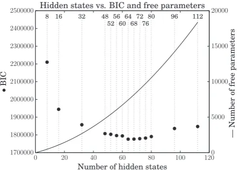
Selecting the Number of Hidden States
Fourteen models were trained (8, 16, 32, 48, 52, 56, 60, 64, 68, 72, 76, 80, 96, and 112 hidden state models). The 64 hidden state model was chosen as the best model, as it had the lowest Bayesian Information Criterion (BIC,fig. 3).
Stationary Distributions over Dihedral Angles Capture
the Empirical Distribution
Figure 4illustrates the sampled and empirical dihedral angle distributions. There is a good correspondence between dihe-dral angles sampled under the model (fig. 4, left) and the empirical distribution of dihedral angles in our training data-set (fig. 4, right) for all three cases illustrated (all amino acids, glycine only, and proline only). The correspondence is not surprising given that ETDBN is effectively a mixture model with a large number of mixture components.
Estimates of Evolutionary Time from Dihedral Angles
Are Consistent with Estimates from Sequence
Whilst ETDBN has a general scope with respect to applica-tions (including acting as proposal distribution or as a build-ing block in a homology modelbuild-ing application), we envision the primary application being inference of evolutionary parameters.Figure 5compares evolutionary times estimated using only pairs of homologous amino acid sequences versus only pairs of homologous dihedral angles. As desired, the two estimates of evolutionary time for each protein pair are similar, as can be seen by the proximity of the points to the identity line.
A pairedt-test gave ap-value of 0.578, thus failing to reject the null hypothesis that there is no difference between branch lengths estimated using sequence only versus angles only. This indicates that there is sufficient evolutionary infor-mation in the dihedral angles to estimate the evolutionary times and that the model is consistent in its estimates, lacking a significant tendency to underestimate or overestimate the evolutionary times when either sequence or dihedral angles are used.
Interestingly, the variance in the sampled evolutionary times is higher when dihedral angles only are used, as com-pared with sequence only (see fig. S1, Supplementary Material online).
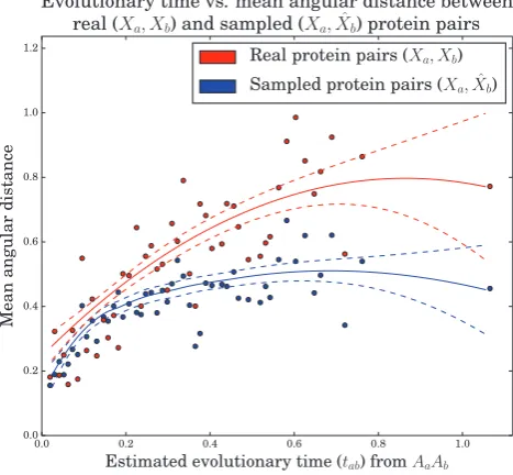
The Relationship between Evolutionary Time and
Angular Distance Is Adequately Modeled
We investigated the relationship between evolutionary time and angular distance between real protein pairs and protein pairs where the dihedral angles of pb (Xb) were treated as missing and hence sampled (fig. 6).
As expected, for both real and sampled pairs, angular dis-tance tends to increase as a function evolutionary time. For larger evolutionary times a plateau begins to emerge, which is expected as the maximum possible theoretical angular dis-tance ispffiffiffi82:828.
When the evolutionary time is exactly zero (tab¼0) under
For small evolutionary times (<0.2) the curves for the real and sampled protein pairs show a good correspondence, however, for larger evolutionary times the model tends to underestimate angular distances. This may reflect the fact that the tpd of the WN diffusion specified is localized around its mean, even when the evolutionary time is large; therefore, dihedral angles distant from this mean are unlikely to be sampled. To a certain extent this is mitigated by the jump model, which occasionally allows for large changes in dihedral angle, but may still be somewhat limited in its flexibility, as jumps can only occur between two site-classes. The majority of protein pairs in our training dataset represent smaller evo-lutionary times (81.7% of evoevo-lutionary times are smaller than 0.4) and therefore protein pairs with larger evolutionary times and their associated jumps are underrepresented in our data-set, which may also explain the underestimation.
An additional possibility is that ETDBN does not attempt to model global dependencies.Echave and Fernandez (2010)
use a LFENM model (which does take into account global dependencies) and provide evidence showing that the ma-jority of structural changes is due to collective global defor-mations rather than local defordefor-mations. A local model such as ETDBN, by definition, does not take into account global de-pendencies and therefore does not fully account for their contribution to structural divergence.
Evaluation of the Model
The conditional independence structure in (eq. 1) enables computationally efficient sampling from the model under different combinations of observed or missing data. For ex-ample, ETDBN can be used to sample (i.e., predict) the dihe-dral angles of a protein from its corresponding amino acid sequence, a homologous amino acid sequence, a homologous set of dihedral angles, the corresponding secondary structure, a homologous secondary structure, or any combination of them.
Predictive accuracy was measured using 38 homologous protein pairs in the test dataset. For every protein pair (pa,pb),
the dihedral angles ofpbin each pair were treated as missing,
[image:8.595.51.286.49.218.2]and these missing dihedral angles were sampled under the model given a particular combination of observation types. The average angular distance between the sampled and known dihedral angles was used as the measure of predictive accuracy.
Figure 7 gives an example of predictive accuracy under different combinations of observations types overlaid on a cartoon structure of the protein structure being predicted, whereasfigure 8provides a representative view of predictive accuracy across 10 different protein pairs in the test dataset for different combinations of observations types. We highlight some of the key patterns identified in figures 7 and 8 as follows.
Combination 1 refers to random sampling from the model, implying no data observations were conditioned on besides the respective lengths of proteins pa and pb. The average
angular distance between the true and predicted dihedral angles was 1.6. Random sampling acts as a baseline for pre-dictive accuracy. It is apparent fromfigure 7that the model has a propensity to predict right-handeda-helices, which is the most populated region in the Ramachandran plot.
Under combination 2, only the amino acid sequence cor-responding topbis observed. As expected infigures 7and8
there is an increase in predictive accuracy with the addition of the amino acid sequence relative to combination 1.
Under combination 3, we add in the amino acid sequence of a homologous protein (pa). In all ten cases there is an
improvement in predictive accuracy. The improvement in predictive accuracy is reasonable, as knowledge of the se-quence evolutionary trajectory is expected to encode infor-mation about structure evolution and hence will inform the dihedral angle conformational possibilities.
Under combination 4, in addition to the two amino acid sequences we treat the homologous secondary structure as observed. This results in a substantial improvement in pre-dictive accuracy as one would expect. Knowledge of the amino acid sequence and a homologous secondary structure strongly informs regions of the Ramachandran plot that are likely to be occupied.
Under combination 5 (which we consider thecanonical combination—the standard homology modeling scenario), we treat both amino acid sequences as observed, as well as the dihedral angles of the homologous protein (pa)—in all
cases the predictive accuracy improves over combination 4. This is anticipated as the homologous dihedral angles are expected to be the best proxy for missing dihedral angles and are therefore expected to be more informative than sec-ondary structure alone. Note that the availability of a homol-ogous amino acid sequence pair here and in combination 4 is consequential as it informs the evolutionary timetab
param-eter, which will typically constrain the distribution over dihe-dral angles and reduce the associated uncertainty.
Finally, in combination 6, the same data observations as in combination 5 are used, except the alignment is treated as given a priori (by the HOMSTRAD alignment)
rather than as unobserved. The HOMSTRAD alignment is based on a structural and sequence alignment ofpaand
pband therefore is expected to encode a higher degree of
homology and structural information than combination 5 (where the alignment is treated as unobserved and
therefore a marginalization over alignments is per-formed). On average, there is a slight improvement in predictive accuracy when fixing the alignment, albeit the magnitude of improvement is not substantial. This demonstrates the accuracy of the alignment HMM.
The alignment HMM accounts for alignment uncertainty in a principled manner, which is particularly useful when an appropriate alignment is unavailable. However, it should be noted that inference scalesOðjpajjpbjh2Þwhen treating the alignment as unobserved. Inference scalesOðmh2Þwhen the alignment is fixed a priori, wheremis the length of alignment Maband is typically much smaller thanjpajjpbj.
It should be emphasized that we do not expect ETDBN to compete with structure prediction packages such as Rosetta (Rohl et al. 2004) or homology modeling software such as
Arnold et al. (2006)in terms of predictive accuracy. Our cur-rent model is a local model of structure evolution—it is not even expected capture fundamental constraints such as the radius of gyration of a protein or other global features typical of proteins.
Evolutionary Hidden States Reveal a Common
Evolutionary Motif
One benefit of ETDBN is that the 64 evolutionary hidden states learned during the training phase are interpretable. We give an example of a hidden state encoding a jump event that was subsequently found to represent an evolutionary motifpresent in a large number of protein pairs in our test and training datasets.
Evolutionary hidden state 3 (fig. 9) was selected from the 64 hidden states as an example of a hidden state encoding a jump event and capturing angular shift (a large change in dihedral angle). A notable feature of this hidden state is that the change in dihedral angles between site-classesr1andr2is associated with specific amino acid changes. In site-classr1the
amino acid frequencies are relatively spread out amongst a number of amino acids, whereas in site-classr2the frequen-cies are particularly concentrated in favor of glycine (Gly) and asparagine (Asp), with glycine being significantly more prob-able in site-classr2thanr1. This suggests that, conditioned on hidden state 3, an exchange between a glycine to another amino acid is likely indicative of a jump and hence a corre-sponding change in dihedral angle. This is consistent with what we find in a subsequent analysis of evolutionary motifs. This particular jump occurs in coil regions.
Having selected hidden state 3, positions in 238 protein pairs were analyzed for evidence of the corresponding evolu-tionary motif. 38 protein pairs in the test dataset and a further 200 from the training dataset were analyzed using the criteria described in the Methods section. Using the first criterion, 84 protein sites in 59 protein pairs corresponding to Hi¼3 (evolutionary hidden state 3) were identified. Of the 84 pro-tein sites, 34 propro-tein sites met the second criterion.
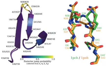
We give an example of a homologous protein pair illus-trating the identified evolutionary motif. Two histidine-containing phosphocarriers, 1pch (Mycoplasma capricolum) and 1poh (Escherichia coli), were identified as having the evo-lutionary motif (fig. 10) at homologous site E39/G39.
FIG. 5. Scatterplot comparing evolutionary times estimated using pairs of homologous amino acid sequences only versus pairs of ho-mologous sets of dihedral angles only forN¼38 proteins pairs in the test dataset. Thex-coordinate of each point gives the estimated evo-lutionary time based only on the amino acid sequence, whereas the
y-coordinate gives the estimated evolutionary time based only on the dihedral angles. The diagonal line representsy¼x.
FIG. 6.Evolutionary time versus angular distances between real and corresponding sampled proteins pairs in the training dataset at 50 representative evolutionary times. Mean angular distances (see ‘Calculation of angular distances’ in the supplementary Material, Supplementary Material online) between the real dihedral angles in a protein pair (red,XaandXb) and sampled dihedral angles in a sampled protein pair (blue,XaandX^b) were compared with test
how well the sampled dihedral angles reproduced the real angular distances. The dihedral angles (^Xb) of each sampled protein pair were
sampled by conditioning on both amino acid sequences and the homologous dihedral angles (Aa,Ab,Xa), and the estimated evolu-tionary time (^tab) for the real protein pair. The regression curves were
[image:10.595.310.544.54.270.2] [image:10.595.49.287.54.271.2]Most positions in the homologous pair have low posterior jump probabilities (0.0), with the exception of positions N38/N38 and E39/G39, which both have high posterior jump probabilities (1.0). The exchange between a gluta-mate (at position 39 in 1poh) and a glycine (at position 39 in 1pch) appears to be responsible for the shift in dihedral angle. This exchange corresponds to a significant jump in di-hedral angle: h/1poh;E39 ;w1pch;E39i ¼ h1:63;0:06i !
h/1poh;G39;w1pch;G39i ¼ h1:40;0:22i. The angular dis-tance between the two dihedral angles is 2.01. This is consistent with the amino acid frequency parameters specified by the two site-classes for hidden state 3 (fig. 9). Site-classr1indicates that a number of amino acids (alanine, aspartic acid, glycine, histidine, lysine, asparagine, proline, glu-tamine, arginine, serine, and theorine) other than glutamate plausibly coincide with the particular dihedral angle confor-mation specified by site-classr1. The involvement of glycine in a jump is not surprising as it is a small and flexible amino acid, whereas the role of asparagine is less clear. In our analysis of 238 protein pairs we found that of the seven positions meeting the criteria for hidden state 3 and involving an exchange with asparagine (Asn), four were an exchange between an
asparagine and a glycine, whereas the remaining three were between asparagine and one of lysine, histidine, or serine.
Using Dihedral Angles for Alignment
A valuable feature of our model is its ability to account for alignment uncertainty by summing over possible pairwise alignments using the TKF92 model as a prior distribution over indel histories, whilst simultaneously taking into account neighboring dependencies amongst aligned sites. Doing so results in a sample of alignments rather than a single align-ment. Nevertheless, a single Maximum A Posteriori (MAP) pairwise alignment may be obtained from the alignment sam-ples and used for downstream analysis.
ETDBN and several other alignment methods (namely StatAlign, BAli-Phy, MUSCLE, and MAFFT) were used to infer pairwise alignments from simulated and real data under var-ious combinations of data observations, for example: an amino acid sequence pair (Aa,Ab), a secondary structure
se-quence pair (Sa,Sb), a dihedral angle sequence pair (Xa,Xb) and combinations thereof.
In the first set of benchmarks (fig. 11A), pairs of proteins were simulated from the ETDBN model conditioned on 38
FIG. 7.Cartoon structure representations ofE. coliglyceraldehyde-3-phosphate dehydrogenase structure (PDB 1gad) are depicted in each panel, overlaid with predictive accuracy when using different combinations of observed data to predict missing dihedral angles in 1gad.Thermus aquaticusglyceraldehyde-3-phosphate dehydrogenase (PDB 1cer) was used as a homolog for the purposes of prediction. Predictive accuracy is indicated using a color gradient depicting the mean angular distance between the true dihedral angle (Xi
1gad) and the predicted (sampled) dihedral angles (^Xi1gad) at each amino acid position. The label at the bottom of each panel indicates the data combination used. In (A), no data was used for prediction. In (B), only the amino acid sequence corresponding to 1gad (A1gad) was used. In (C), the amino acid sequence of 1gad (A1gad) and the
amino acid sequence of the homologous protein (A1cer) were used. In (D), both amino acids sequences (A1cerandA1gad) and the secondary
structure of the homologous protein (S1cer) were used. In (E), both the amino acid sequences (A1cerandA1gad) and the dihedral angles of the
homologous protein (X1cer) were used. Finally, in panel (F) the same combination of observations was used as in (E), but the alignment was treated
[image:11.595.50.552.49.343.2]FIG. 8.Benchmarks of predictive accuracy (measured using angular distance, lower is better) on a random subset of ten protein pairs in the test dataset, giving a representative view of predictive accuracy under six different combinations of observations. The dihedral anglesXbofpbwere treated as missing and were sampled under the model, whereaspawas a homologous protein used for the purposes of prediction. See the legend of
figure 7for a description of each combination (A–F). The final set of bars, denoted ‘Mean (N¼38)’, are the mean values for the entire test dataset of
N¼38 protein pairs. The error bars are the standard errors.
different pairwise alignments and corresponding evolutionary times. This resulted in a set of 38 simulated pairwise align-ments together with corresponding observations, implying that the true underlying alignments were known for each of the simulated protein pairs. ETDBN and a number other alignment methods were used to infer pairwise alignments for each. The alignment similarity metric (Schwartz et al. 2005) was used to measure the similarity between the inferred alignments and the true alignments, where higher similarity indicates better predictions. It was found that, when using the simulated amino acid sequences alone, ETDBN (11A.5) out-performed all four other methods tested (11A.1 MUSCLE, 11A.2 MAFFT, 11A.3 StatAlign and 11A.4 BAli-Phy). However, the greater performance of ETDBN compared with other methods cannot be considered a fair comparison, as the data were simulated under the ETDBN model.
More revealing infigure 11Awas the alignment similar-ity under ETDBN when using different combinations of simulated data observations. It was found that secondary structure alone (11A.6) performed the worst, which is un-surprising given that only three states were available to align the proteins. The second worst in terms of alignment similarity was amino acid sequences alone (11A.5), fol-lowed by amino acid sequences and secondary structures (11A.7). Interestingly, using dihedral angles only (11A.8) outperformed both 11A.5 (sequences only) and 11A.6 (sec-ondary structures only). Finally, using amino acid sequence together with dihedral angles (11A.9) or all three data types combined (11A.10) outperformed all other combi-nations. This illustrates that, at least under simulation
conditions, increasing the number of data observations results in better alignment accuracy.
Following that, the various alignment methods were benchmarked against 38 pairwise alignments consisting of real sequence and structure observations in the test dataset. These pairwise alignments were obtained from the HOMSTRAD alignments. The sequence identity of these pair-wise alignments ranged from 10% to 93%, with an average sequence identity of 39%. In addition to methods 1–10 in
figure 11A, five structural alignment methods were also used: 11. StatAlign (Herman et al. 2014), 12. TMAlign (Zhang and Skolnick 2005), 13. Mammoth (Ortiz et al. 2002), 14. Dali (Holm and Rosenstro¨m 2010), and 15. CE (Shindyalov and Bourne 1998). These methods were not used in 11A due to the lack of an appropriate model for simulating the evolution of three-dimensional protein structures.
When benchmarking the MAP estimated alignments against the HOMSTRAD alignments (fig. 11B), using real se-quences alone for inference (Aa,Ab), ETDBN (11B.5) had a
similar degree of accuracy when compared with several other sequence-based methods (11B.1 StatAlign, 11B.2 BaliPhy, 11B.3 MUSCLE, and 11B.4 MAFFT). This demonstrates that ETDBN has performance comparable to that of other commonly-used sequence alignment methods.
Using (Sa,Sb) alone, ETDBN (11B.6) had substantially lower
alignment similarity compared with sequence only, which was expected given that a similar result was obtained for the simulated data (11A.6). However, when including the real sequences (11B.7) the predictive accuracy was once again comparable to sequence only inferences (11B.1–11B.5).
[image:13.595.81.512.48.317.2]When using (Xa,Xb) alone (11B.8), the alignment similarity
was found to be somewhat worse than the sequence only cases. Furthermore, when introducing the sequences (11.9) and secondary structures (11B.10) in addition to the dihedral angles, the similarity remained worse than the sequence only methods (11B.1–11B.5), despite the additional information. These results are in contrast to the results we obtained for simulated data (11A.8–11A.10).
The non-statistical structural alignment methods (11B.12– 11B.15) faired the best, likely because they use a criteria similar to that used to align the HOMSTRAD alignments. When interpreting these results it is important to note the HOMSTRAD alignments should not be considered the true underlying alignments and may even be strongly biased. For example, they may favor the closest structural superimposi-tion of structures or the most parsimonious alignments, with the fewest number of indels. In the evolutionary modeling context our goal is to distinguish between homologous sites (sites that have evolved via mutation alone) and indels. In practice, it is extremely difficult to obtain the true underlying alignment (sets of homologies and indels), because it would require an experiment where every indel event since the common ancestor is observed, a seeming impossible task outside of simulation or laboratory conditions.
After further investigation, the trend of lower alignment similarity seen in figure 11B.6–11B.10 when using ETDBN with structural observations compared with sequence only or non-statistical structural alignment methods was found to reverse (11C.6–11C.10) upon calculating the precision of predicting homologous sites (the fraction of sites which were predicted as homologous and were correctly predicted as such). Therefore when only dihedral angle observations are used, ETDBN underpredicts the number of homologous sites, how-ever, when a homologous site is predicted, it is correctly pre-dicted more often than when using only amino acid sequences. In particular, ETDBN predicted fewer homologous sites with coiled secondary structure compared with homol-ogous sites with helical or sheet secondary structure. This pattern of results may be in part due to the WN diffusion used to model evolution of dihedral angles. The WN diffusion is suitable for modeling angular drift (small changes in angles localized around a region of the Ramachandran plot) but does not sufficiently capture angular shift (large changes in angles between regions of the Ramachandran plot, which are more likely in coiled regions) due to stationarity. As noted before, the jump model is an abstraction intended to capture the end-points of evolution by allowing a jump between two regions of the Ramachandran plot, abstracting a potential intermediate evolutionary trajectory for the sake of compu-tational tractability. Note that the jump model accurately captures the common cases where a single mutation induces a large conformational shift.
Concluding Remarks
The main achievement of this work is a computationally tractable, generative and interpretable probabilistic model of protein sequence and structure evolution on a local scale. A
B
C
Previous stochastic models of protein sequence and struc-ture evolution emphasized estimation of evolutionary param-eters (Challis and Schmidler 2012; Herman et al. 2014). ETDBN is somewhat of a departure from these previous models, but is likewise capable of estimating evolutionary parameters. We show that estimates of evolutionary times inferred under ETDBN are consistent regardless of whether amino acid sequence or dihedral angle observations are used. In addition, the relationship between evolutionary time and angular distance in real proteins is adequately recapitulated in protein pairs sampled under the model, albeit the angular distance is underestimated for larger evolutionary times, which might be explained by the limited flexibility of the jump model and the lack of taking into account global dependencies.
Like previous models, ETDBN is capable of dealing with alignment uncertainty by marginalizing over indel histories; it predicts pairwise MAP consensus alignments with accuracy similar to that of score-based and statistical alignment methods.
The generative nature of ETDBN allows us to demonstrate that the underlying empirical distributions over dihedral an-gles (depicted using Ramachandran plots) are captured and that the model is capable of predicting missing observations, such as dihedral angles, from a variety of different data types. For example, an amino acid sequence, a homologous amino acid sequence, a homologous secondary structure, a homol-ogous set of dihedral angles, or any combination thereof.
Based on its local nature, ETDBN does not constitute a homology modeling method in itself. Rather, it can be used as a building block, much like fragment libraries model local structure in protein structure prediction methods. ETDBN places the homology modeling problem on a statistical foot-ing, enabling a number of approaches to later be used, such as multi-level modeling, that is, combining fine-grained distribu-tions (for example, distribudistribu-tions over dihedral angles, such as ETDBN) and coarse-grained distributions (for example, distri-butions describing the global properties of proteins, such as compactness). In particular, a method referred to as ‘the Reference Ratio method’ can be used to combine fine-grained and coarse-fine-grained distributions in a statistically prin-cipled manner (seeFrellsen et al. 2012;Hamelryck et al. 2010). However, we have shown that the current model can already be used for the inference of evolutionary parameters in its present form.
In addition to multi-level modeling, probabilistic models such as ETDBN allow one to account for and to make state-ments about uncertainty (e.g. with respect to evolutionary time, alignment, etc.) in a rigorous manner. In principle, ETDBN, like TorusDBN (Boomsma et al. 2008), could be used as a proposal distribution. In other words, ETDBN could be used to sample protein structures (possibly conditioned on various data observations) in a computationally efficient manner, such that the resulting samples are expected to be located in regions of high probability density with respect to the true underlying distribution.
A final key feature of our evolutionary model is its inter-pretable nature. This interpretability enables the
identification of potential evolutionary motifs—common patterns of sequence–structure evolution. We identify one such evolutionary motif in 34 different homologous protein pairs. A major direction for future research is the further identification of such evolutionary motifs. Understanding these evolutionary motifs, may 1) improve homology mod-eling predictions; 2) provide more accurate estimates of evo-lutionary parameters; and 3) produce better models of protein evolution that more realistically capture evolutionary trajectories through sequence and structure space, which may help identify functionally relevant positions that are po-tential drug targets.
Future Challenges
Pairwise to Phylogeny
For reasons of computational tractability the implemented model is pairwise, but it is theoretically possible to generalize it to a phylogeny, such as inHerman et al. (2014). In practice, for three or more sequences on a phylogeny it is necessary to marginalize out the unobserved ancestral protein states in order to compute likelihoods. Felsenstein’s algorithm can be used to marginalize over discrete ancestral states, such as amino acids in a computationally efficient manner. However, we do not know whether a similar efficient algo-rithm exists for marginalizing the continuous ancestral dihe-dral angle states under the WN diffusion, thereby necessitating a more expensive MCMC algorithm. A possibly greater computational hindrance to considering a phylogeny is the alignment problem, which scales Oðl1l2. . .lNÞ, where liis the length of sequencei
and N is the number of sequences, although MCMC approaches are possible (Herman et al. 2014).
Context-Dependence
Although we believe our model provides a substantial im-provement over current stochastic models of sequence and structural evolution, there is still scope for improvement. The WN diffusions used to model dihedral angle evolution ade-quately capture angular drift (small local changes in dihedral angle), but are less capable of capturing angular shift (large changes in dihedral angle). This is to a considerable extent mitigated by the introduction of jump events, as discussed before. A more realistic model would model the entire evo-lutionary trajectory, allowing an arbitrary number of switches between site-classes together with neighboring dependencies amongst adjacent sites along the evolutionary trajectory. Similar context-dependent models are typically computa-tionally expensive and require sophisticated inference proce-dures (Robinson et al. 2003;Yu and Thorne 2006).
Software Availability
Supplementary Material
Supplementary material are available atMolecular Biology and Evolutiononline.
Acknowledgments
The authors acknowledge funding from the University of Copenhagen 2016 Excellence Programme for Interdisciplinary Research (UCPH2016-DSIN). The second au-thor acknowledges support from project MTM2016-76969-P from the Spanish Ministry of Economy and Competitiveness and ERDF. Authors acknowledge valuable comments from three referees that led to substantial improvements in the manuscript, as well as initial discussions with Christian Havn, Ian Lim and Mathias Cronj€ager.
References
Arnold K, Bordoli L, Kopp J, Schwede T. 2006. The SWISS-MODEL work-space: a web-based environment for protein structure homology modelling.Bioinformatics22(2):195–201.
Boomsma W, Mardia KV, Taylor CC, Ferkinghoff-Borg J, Krogh A, Hamelryck T. 2008. A generative, probabilistic model of local protein structure.Proc Natl Acad Sci U S A. 105(26):8932–8937.
Boomsma W, Tian P, Frellsen J, Ferkinghoff-Borg J, Hamelryck T, Lindorff-Larsen K, Vendruscolo M. 2014. Equilibrium simulations of proteins using molecular fragment replacement and NMR chemical shifts.
Proc Natl Acad Sci U S A. 111(38):13852–13857.
Challis CJ, Schmidler SC. 2012. A stochastic evolutionary model for pro-tein structure alignment and phylogeny. Mol Biol Evol. 29(11): 3575–3587.
Echave J. 2008. Evolutionary divergence of protein structure: the linearly forced elastic network model.Chem Phys Lett. 457(4):413–416. Echave J, Fernandez FM. 2010. A perturbative view of protein structural
variation.Proteins: Struct Funct Bioinform. 78(1):173–180.
Edgar RC. 2004. MUSCLE: multiple sequence alignment with high accu-racy and high throughput.Nucleic Acids Res. 32(5):1792–1797. Felsenstein J. 1985. Phylogenies and the comparative method.Am Nat.
125(1):1–15.
Frellsen J, Mardia KV, Borg M, Ferkinghoff-Borg J, Hamelryck T. 2012. Towards a general probabilistic model of protein structure: the ref-erence ratio method. In: Bayesian methods in structural bioinfor-matics. New York: Springer, p. 125–134.
Garcıa-Portugue´s E, Sørensen M, Mardia KV, Hamelryck T, 2017. Langevin diffusions on the torus: estimation and applications. arXiv:1705.00296.
Gilks WR, Richardson S, Spiegelhalter D. 1995. Markov chain Monte Carlo in practice. London: CRC Press.
Grishin NV. 1997. Estimation of evolutionary distances from protein spatial structures.J Mol Evol. 45(4):359–369.
Grishin NV. 2001. Fold change in evolution of protein structures.J Struct Biol. 134(2):167–185.
Gutin AM, Badretdinov AY. 1994. Evolution of protein 3D structures as diffusion in multidimensional conformational space. J Mol Evol. 39(2):206–209.
Halpern AL, Bruno WJ. 1998. Evolutionary distances for protein-coding sequences: modeling site-specific residue frequencies.Mol Biol Evol. 15(7):910–917.
Hamelryck T, Borg M, Paluszewski M, Paulsen J, Frellsen J, Andreetta C, Boomsma W, Bottaro S, Ferkinghoff-Borg J. 2010. Potentials of mean force for protein structure predic-tion vindicated, formalized and generalized. PLoS ONE. 5(11):e13714.
Herman JL, Challis CJ, NovakA, Hein J, Schmidler SC. 2014. Simultaneous Bayesian estimation of alignment and phylogeny under a joint model of protein sequence and structure. Mol Biol Evol. 31(9):2251–2266.
Holm L, Rosenstro¨m P. 2010. Dali server: conservation mapping in 3D.
Nucleic Acids Res. 38(Web Server issue):W545–W549.
Katoh K. et al. 2002. MAFFT: a novel method for rapid multiple sequence alignment based on fast Fourier transform. Nucleic Acids Res. 30(14):3059–3066.
Koshi JM, Goldstein RA. 1998. Models of natural mutations including site heterogeneity.Proteins32(3):289–295.
Lartillot N, Philippe H. 2004. A Bayesian mixture model for across-site heterogeneities in the amino-acid replacement process. Mol Biol Evol. 21(6):1095–1109.
Lio P, Goldman N, Thorne JL, Jones DT. 1998. PASSML: combining evo-lutionary inference and protein secondary structure prediction.
Bioinformatics14(8):726–733.
Miklos I, Lunter G, Holmes I. 2004. A long indel model for evolutionary sequence alignment.Mol Biol Evol. 21(3):529–540.
Mizuguchi K, Deane CM, Blundell TL, Overington JP. 1998. HOMSTRAD: a database of protein structure alignments for homologous families.
Protein Sci. 7(11):2469–2471.
Ortiz AR, Strauss CE, Olmea O. 2002. Mammoth (matching molecular models obtained from theory): an automated method for model comparison.Protein Sci. 11(11):2606–2621.
Robinson DM, Jones DT, Kishino H, Goldman N, Thorne JL. 2003. Protein evolution with dependence among codons due to tertiary structure.
Mol Biol Evol. 20(10):1692–1704.
Rohl CA, Strauss CE, Misura KM, Baker D. 2004. Protein structure pre-diction using Rosetta.Methods Enzymol. 383:66–93.
Schwartz AS, Myers EW, Pachter L. 2005. Alignment metric accuracy.
arXiv preprint q-bio/0510052.
Shindyalov IN, Bourne PE. 1998. Protein structure alignment by incre-mental combinatorial extension (CE) of the optimal path.Protein Eng. 11(9):739–747.
Siepel A, Haussler D. 2004. Combining phylogenetic and hidden Markov models in biosequence analysis. J Comput Biol. 11(2–3):413–428.
Thorne JL, Kishino H, Felsenstein J. 1992. Inching toward reality: an im-proved likelihood model of sequence evolution. J Mol Evol. 34(1):3–16.
Whelan S, Goldman N. 2001. A general empirical model of protein evolution derived from multiple protein families using a maximum-likelihood approach.Mol Biol Evol. 18(5):691–699. Yu J, Thorne JL. 2006. Dependence among sites in RNA evolution.Mol
Biol Evol. 23(8):1525–1537.
Zhang Y, Skolnick J. 2005. TM-align: a protein structure alignment
algorithm based on the TM-score. Nucleic Acids Res.