Location Prediction Optimisation in Wireless Sensor Networks Using Kriging Interpolation

White Rose Research Online URL for this paper:

http://eprints.whiterose.ac.uk/100053/

Version: Accepted Version

Article:

Ali, A., Ikpehai, A., Adebisi, B. et al. (1 more author) (2016) Location Prediction

Optimisation in Wireless Sensor Networks Using Kriging Interpolation. IET Wireless

Sensor Systems, 6 (3). pp. 74-81. ISSN 2043-6386

https://doi.org/10.1049/iet-wss.2015.0079

This paper is a postprint of a paper submitted to and accepted for publication in IET

Wireless Sensor Systems and is subject to Institution of Engineering and Technology

Copyright. The copy of record is available at IET Digital Library

[email protected] https://eprints.whiterose.ac.uk/

Reuse

Unless indicated otherwise, fulltext items are protected by copyright with all rights reserved. The copyright exception in section 29 of the Copyright, Designs and Patents Act 1988 allows the making of a single copy solely for the purpose of non-commercial research or private study within the limits of fair dealing. The publisher or other rights-holder may allow further reproduction and re-use of this version - refer to the White Rose Research Online record for this item. Where records identify the publisher as the copyright holder, users can verify any specific terms of use on the publisher’s website.

Takedown

If you consider content in White Rose Research Online to be in breach of UK law, please notify us by

Location Prediction Optimisation in WSN Using

Kriging Interpolation

Arshad Ali

, Augustine Ikpehai

, Bamidele Adebisi

, Lyudmila Mihaylova

_{Islamic University Al Madinah Al Munawarah, Saudi Arabia}

2

_{Division of Electrical and Electronic Engineering, Manchester Metropolitan University, Manchester, UK.}

_{Department of Automatic Control and Systems Engineering, University of Sheffield, UK}

[email protected]

_{, [email protected]}

_{, [email protected]}

_{, [email protected]}

Author to whom correspondence should be addressed: [email protected]

ABSTRACT

Many wireless sensor network (WSN) applications rely on precise location or distance information. Despite the potentials of WSNs, efficient location prediction is one of the subsisting challenges. This paper presents novel prediction algorithms based on a Kriging interpolation technique. Given that each sensor is aware of its location only, the aims of this work are to accurately predict the temperature at uncovered areas and estimate positions of heat sources. By taking few measurements within the field of interest and by using Kriging interpolation to iteratively enhance predictions of temperature and location of heat sources in uncovered regions, degree of accuracy is significantly improved. Following a range of independent Monte Carlo runs in different experiments, it is shown through a comparative analysis that proposed algorithm delivers approximately 98% prediction accuracy.

Index Terms

wireless sensor network, sensor location management, node position interpolation, Kriging, location prediction.

I. INTRODUCTION

Emerging infrastructures such as smart grids and Internet of Things (IoT) will rely on sensors to determine precise location of targets as a precursor to more advanced operations such as automation and control. Therefore, the need for efficient prediction techniques in WSNs cannot be over-emphasized. Considering that they run on batteries, wireless sensors are typically designed with low complexity and limited energy. Sensors are particularly suitable for environments considered unsafe for human occupation and where other wireline solutions have either failed or are not feasible. On a large scale, WSNs are also used for surveillance in utility, industrial environment, military, healthcare, transportation, volcano, earthquake monitoring and has been recently proposed for the smart grid. As the size of the field increases, the number of sensors required to provide adequate coverage increases in a corresponding proportion.

Fig. 1 illustrates a WSN deployment scenario in which sensor nodes form adjacency with their neighbours. Each node has a limited transmission range, hence a transmission from a sensor node to the control server typically consists of a combination of strong (solid lines) and weak (broken lines) communication paths arising from the intermediary nodes towards the destination. For a small field size (e.g. in-house or within an office space), the position of heat source and temperature at different points can be meticulously determined. However, that is not feasible for large-scale deployment involving hundreds of thousands or millions of nodes. The result is that for large fields, nodes are randomly deployed and as expected, there are regions in the field where nodes are either too close to each other or too far apart. Without losing sense of generality, the words sensor node, sensor and node are interchangeably used in this paper.

Figure 1:Wireless Sensor Network

intrusion detection [1] and location of victims in search and rescue operation [2] require accurate location detection. It will therefore be rewarding to have efficient techniques for accurately detecting object location in large fields. Using the Kriging interpolation technique, new location prediction algorithms are demonstrated and proposed in this paper as shown in Algorithms 1 and 2. By that, answers are provided to the following questions: (i) how many sensor nodes are actually needed in a given field, (ii) how can sensor’s locations be optimally determined (iii) is it possible to achieve adequate coverage with less number of sensors, (iv) is it possible to dynamically measure physical quantities at different locations with the same sensors.

References [3] and [4] attempt to provide answers to some of these questions through numerical results and quantitative analysis of simulations results respectively. Despite the benefits of WSNs, the unpredictable nature of the wireless medium coupled with the short communication range sometimes renders their performance inadequate and anticipated level of service unattainable. Noise affects WSN operations generally, as received signal strength indicator (RSSI) degrades in the presence of noise. Independent location estimation is therefore a possible option, from economic and operational standpoints.

The aim of this work is to improve coverage efficiency by taking advantage of spatial correlation of temperature at different spots within the field and combining that with an interpolation technique to estimate temperature and locations of heat sources in regions without WSN coverage. By using fewer nodes, network traffic can be reduced and the effect of noise on location estimation can be significantly reduced.

The main contribution of this work is exploitation of Kriging interpolation to enhance prediction of two key physical quantities; temperature in uncovered locations and positions of heat sources. This will enhance coverage efficiency generally and reduce cost of communication in particular. The rest of this paper is organised as follows. Section 2 provides a brief overview of related work while experimental setup employed in this work is described in section 3. In section 4, the various sensor relocation strategies and performance of the proposed system are discussed. The key contributions of this paper are summarised in section 5.

II. MOTIVATION AND RELATED WORK

It was found in [5] that parameters such as the distance between nodes, network topology, the routing algorithm, transmission power, network capacity, data encoding, modulation scheme, channel radio frequency (RF), bandwidth and channel access affect the overall power consumption in WSNs in different proportions. In an attempt to provide some insight into these, several authors have studied the node location management in WSNs. For example, the authors of [6] formulated it as a distributed set of localization problems and employed an algorithm in which reference nodes (anchor nodes) were assumed to have prior knowledge of their positions in the field to derive relationship between Received Signal Strength Indicator (RSSI) [7] and the relative distance between pairs of nodes. Other ranging techniques using difference of arrival (TDoA), angle of arrival and time of arrival have also been studied [8].

Limitations of these methods include: (i) the assumption may not always hold for industrial deployments, (ii) delayed convergence of measurements among sensors, (iii) a large number of nodes required for redundancy in measurements, (iv) the accuracy depends on field geometry. A point within the field is said to be covered if it falls within the transmission range of at least a sensor node. However, in large fields where sensors are randomly deployed, far more nodes are deployed than necessary giving rise to redundancy that may not be needed [9]. Deterministic approaches have been studied in [10], [11] to use minimum number of nodes such that any node n (n™N) is connected tok nodes where 16K 6N. These methods are generally unsuitable for large deployments given that deployment of large number of sensor nodes is often a stochastic process.

Different prediction methods and algorithms have been proposed for location estimation in [12], [13], [14], [15] some of which combine location prediction with selective activation of nodes[11]. Hence, efficient coverage with a minimum number of nodes is still an open research area. In this paper, the spatial correlation of temperature is combined with an interpolation technique to estimate the average temperature at uncovered locations and heat source positions within the field. The use of distributed estimation techniques to predict measurements of unmonitored regions is well documented [16].

While [17] , [18] showed that the Kriging method is unbiased and minimises estimation variance, it is also worthy of note that applications of Kriging interpolation method in geoscience and remote sensing abound in literature [19], [20], [21], [22], [23]. The inspiring work in [22] combines data aggregation (sum of squared difference) with Kriging interpolation to improve estimates at unmonitored locations. In our case, polynomial prediction is combined with Kriging interpolation to improve estimations. The idea is to combine spatial correlation of measured values with a refined process of interpolation to estimate temperature and distance information of heat sources in uncovered regions in the field. This will result in deployment of fewer sensors.

Kriging is geostatistical technique that exploits correlation of physical phenomena or measured values in the same vicinity and interpolate measurements at unmonitored locations [24]. Rather than geographic distance, Kriging relies on statistical distance defined as a function of samples of a phenomenon and the distance between the sampled locations. The variogram is a measure of statistical distance.

Consider a field with temperature distribution such thatZ(x)represents the temperature at locationx. At a distanceh, the variogram can be expressed as

Ψ(x0) = 1

2N(h)

X

N(h)

[Z(x)−Z(x+h)]2. (1) Where N(h) is the number of data pairs at distance h. The spatial correlation in temperature can be observed by computing the variogram for different locations. Assume that a spatial distribution Z of temperature is represented by

Z(x0), Z(x1), ..., Z(xN)at locationsx0, x1,..., xN then the Kriging interpolator at a pointx0 is given by

ˆ

Z(x0) =

N X

i=1

whereλi is the Kriging weight, such that

N X

i=1

λi= 1. (3)

and expected error satisfies

EhZˆ(x0)−Z(x0)

i

= 0. (4)

III. EXPERIMENTALSETUP

All experiments carried out in this paper are based on simulations. For experimental purposes, anM XM square metre area of interest is created and subdivided into a finite number of hexagons. Ideally, the sensor network should be able to monitor the entire environment by combining measurements from its constituent sensor nodes. However, for large fields, adequate coverage requires a large number of sensor nodes; that is costly and energy demanding.

In this work, the proposed system overcome that problem by employing less number of “pseudo-mobile” nodes such that each node dynamically carries out measurements for multiple locations by interpolation. The physical phenomenon monitored is the average temperature. At the beginning of the study, heat sources are stationary and the temperature in the experimental field is assumed fixed. To model the spatial distribution of the temperature, n number of heat sources are placed in the experimental field and each is deployed at centre of the hexagon as shown in Fig. 2. Each heat source

Hi,i=1....nis assumed to create a Gaussian-distributed temperature centred on positionAi, with a mean temperatureTiand

a standard deviation σi. Following Gaussian distribution, the temperature at any point K = (x, y), with one heat source

can be expressed as:

TAi=Ti∗

₁

√ 2πσi

exp−

|Ai−K|2

2σ2

i

. (5)

Therefore, the average temperatureT at any point K withnnumbers of heat sources is given as:

T = 1

n

n X

i=1

TAi. (6)

In this work, the number of sensors is four, the number of heat sources is four and the field dimension is 200 m x 200 m. Furthermoremmoving sensor nodes are randomly deployed in the experimental field and each sensor node is considered to be deployed at centre of the hexagon. Each node uniformly makes several measurements inside a hexagon with half the diagonal taken to be the sensing range.

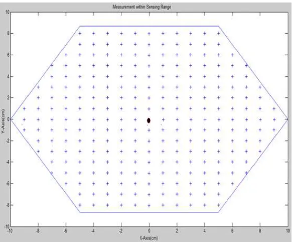
Fig. 3 shows the hexagonal structure of a coverage cell and potential positions for temperature measurements. Hexagon centres define possible positions of the deployed sensor node. The main reason for choosing the hexagon is that the honeycomb structure provided by hexagons allows entire coverage of region of interest, better than triangles and quad-rilaterals [25], [26]. In addition, the sensor node’s movement is constrained to the six neighbouring hexagons around its current position. Each sensor takes several measurements at the centre of the hexagon and uses them to calculate the average temperature. To reduce transmission across the network, each node sends the average temperature to its neighbours by broadcast. Neighbours integrate received information into their memory tables and use Kriging method to interpolate temperature of uncovered regions.

Figure 2: 2D view of spatial distribution of temperature

Figure 3:Measurement locations in a hexagon

determines area of interest in the experimental field based on the interpolated information and finally, Euclidean distance is calculated between the node’s current location and the position of interest. After locating the position for the next move based on a distance vector, the sensor node is moved one step closer to that position. This iterative process continues until a condition of error convergence to a floor value is reached.

IV. SENSOR LOCATION SCHEMES

A. Minimax Temperature

maximum to minimum). ThenP% of Maxima and Minima are chosen from the predicted values and used for sensor node relocation in the experimental field. Each sensor node selects its next target location from that selectedP% predicted values and the sensor node that is nearest to maximum value in the selected P% moves one step closer to the selected target. The selected target is eliminated from the target vector and all its entries are removed from target array that is within the defined threshold(2∗Srange)distance, before the next sensor node selects its target for relocation.

When all sensor nodes select their targets, at the new locations, measurements are repeated and integrated with the existing information in the memory. The same strategy is used when the sensor nodes are divided into two groups, called Maxima and Minima. Each sensor node measures the distance from its current position to the target position that is selected from the predicted data. The sensor closest to the top value on the Maxima or Minima list moves one step closer to the target location. The corresponding group flag is added to its previous value. If the defined number of sensor nodes in the group has already been attained, the corresponding target group is removed from the target selection process. This process continues until the last sensor node selects its target. The Mean Square Error is calculated to measure the performance of the system. The whole process is repeated until the entire area is visited.

B. Minimax Absolute Error

After performing Kriging interpolation in the uncovered area, the absolute error is calculated at common locations between two consecutive iterations. The P% of Maxima and Minima is chosen from the absolute error table for sensor relocation. This selectedP% entries are used for sensor node positioning to gather more information about the field. Each sensor node selects its target from the target array. The target selection is distance-based and each node selects the target that is the closest to its current position. The selected target is eliminated from the target vector and all the entries within the threshold (2∗Srange) distance are removed from the target array before the next sensor node selects its target for

movement and checks the distance between selected targets. If the distance is less than T H (a specified threshold), the node selects a new target from the remaining list and this process continues until the last sensor node selects its target. When all the sensor nodes have moved to new location, each of them takes measurement and all the steps are repeated until entire field is measured. Similar to subsection A, sensor nodes are divided into Maxima and Minima groups in which each node measures distance from its current position to entries listed in the target array. The node closest to the highest value in both groups moves a step closer to the target location. As each node selects its target, its corresponding group increments the group flag by 1 and once the defined number of flag count is reached, the group is considered full and deleted from the target list to prevent other sensors from selecting it. The following performance measures are used to evaluate sensor nodes in the experimental field.

AAE= 1

n

n X

i=1

|T_ip

−1−T

p

i|. (7)

AAEi= 1

nk   1 n nk X j=1 n X i=1

|(T_ip

−1−T

p i)|



. (8)

Where AAE is absolute average error, T_ipis the predicted temperature from current iteration, T_ip

−1is the predicted

temperature from previous iteration, nis the number of data values andnk the total number of simulations. Thus,AAEi

is the AAE over nksimulations.

C. Manual Relocation

Algorithm 1 Error-based sensor node relocation Algorithm: Error based Algorithm (Grid, {s1,s2, ..., sm}

1- set loops = 0; 2- Forsi_{s1,s2, ..., s}

3- Measure Temperatures

T = 1_nPn_i=1TAi

4- Forsi _{s1,s2, ..., sm}broadcast currentT(x, y)

5- Perform Kriging si_{s1,s2, ..., sm}

ˆ

Z(x0) =Pni=1(λiZ(xi))

6- Find mean square error MSE = _n1Pn_i=1(Tt i −T

p i)

2

7- Calculate AAE

AAE= 1

n Pn

i=1 T

p i−1−T

p i

8- For all nodes si_{s1,s2, ..., sm}, locate Max_Error

9- Claculate energy of the system

E₋M₋P =

Pk j=1(T

m j )

2 Pf

i=1(Tft) 2

10- Move one step closer to target 11- End; End;

Algorithm 2 Collaborative location prediction in dynamic environment Algorithm: (Grid,{s1,s2, ..., s} wheremis the number of sensor nodes

1- Deploy heat source ({h1, h2, ..., hn})

2- Deploy nodes randomly ({s1,s2, ..., sm})

3- Take measurement for all ({s1,s2, ..., sm})

4- set loops= 0; set M axLoops=M AXLOOP S; 5- Calculate Average_Temp for all ({s1,s2, ..., sm})

6- Broadcast to all ({s1,s2, ..., sm})

7- Accept & integrate for all ({s1,s2, ..., sm})

8- Move heat source ({h1, h2, ..., hn})

9- Estimate measured locations

10- Predict heat source next location by using polynomial prediction 11- Perform Kriging interpolation in uncovered area.

12- Define Maxima

13- Move Sensor nodes to new location

14- Calculate distance based measure of measure

D. Maximum Absolute Error

Each node performs interpolation for unknown regions and calculates the absolute error at common locations of the predicted temperature between two consecutive iterations.P% of the maximum error is selected from the absolute error table for sensor node relocation. Each sensor node selects its target from a selected target list. Same algorithm outlined in subsection A is repeated until the corresponding group is full and removed from the target list.

The algorithm for sensor nodes relocation in the global view is given in 1.

WhereSi is any node within the sensor set{s1,s2, ..., sm},Ti is the true temperature at any point, Pi is the predicted

values of temperature any point, Zˆ(x0) is the Kriging prediction, λ is the Kriging weight, m is the number of sensor

nodes,E₋M₋P is the energy as a measure of performance,Tm

j is the measured temperature in each iteration andTft is

the true temperature.

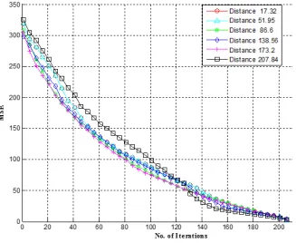
Figure 4: MSE (o_C2_{) vs No of iterations (for different threshold distances)}

V. SYSTEMPERFORMANCE

A. Static Environment: Error-Based Measure of Performance

1) Mean Square Error for Different Threshold Distances: To assess the performance of proposed algorithms for sensor node positioning in experimental field, a mean square error (MSE) is used as performance metric. The MSE is defined as

M SE = 1

n

n X

i=1

T_it−T_iP2

. (9)

whereT_ipis the current predicted temperature, Tt

i is the true temperature and n is the number of predicted values per

iteration (n varies between iterations; decreasing by 4).

In Fig. 4, the variation of MSE with number of iterations is presented for different values of the threshold distance. To avoid bias in the designed algorithm and analysis of results, simulations were carried out several times. In addition, to prevent sensor positions from overlapping, a different threshold distance between the sensor nodes is defined and the algorithm is simulated several times with different initial positions. From Fig. 4, it is evident that the MSE between the actual and predicted temperature values decreases almost exponentially as the number of iterations increases. The same trend is observed for various threshold distances. These observations are reasonably true given that sensors acquire more information about the field as the number of iterations increases from 50 to 250. Such information is used to refine or enhance the prediction of temperature from the polynomial. Hence, it is understandable that the algorithm performed better at higher number of iteration than lower ones. Above 200 iterations, the MSE is generally reduced by around 97% for all investigated scenarios.

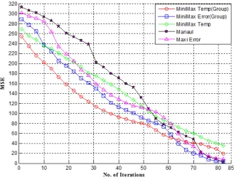
Figure 5: MSE (o_C2_{) vs No of iterations (for various relocation schemes)}

nodes are not allowed to revisit locations within the field. Fig. 5 shows the MSE variation with the number of iterations for different sensor relocation schemes as discussed in section 4.

At the beginning, sensor nodes have little information about experimental field; therefore, interpolation of the uncovered area is poor and the mean square error relatively high. As the simulation progresses, more information is acquired during sensor visit to new locations and new information combined with the previous ones in their memory tables are used to interpolate temperature of areas beyond sensor coverage. The Kriging algorithm continuously improves its predictions and interpolation of the uncovered area and produces higher accuracy as number of iteration increases. Fig. 5 shows a steady reduction in MSE as the number of measurement increases. For instance, it shows a minimum error reduction of 46% (Minimax Temp) between iterations 1 and 40. At iteration 80, Kriging yielded minmum error reduction of 85.19% (Minimax Temp) and maximum of 97.3% (Maxi Error).

3) Mean Square Error Variation with Number of Cells : To observe the effect of the number of cells on measurement accuracy, the MSE for different numbers of cells in the field is calculated. Again, to eliminate bias in the measurements, 100 experiments are conducted per measurement and the average value is taken. The result is presented in Fig. 6.

(a)MSE (o_C2

) vs No of cells (without revisit) (b)MSE (o_C2

) vs No of cells (with revisit) Figure 6:MSE vs No of cells

B. Dynamic Environment: Distance-Based Measure of Performance

1) Distance between Actual and Predicted Heat Source: This subsection begins by transforming the field into a dynamic

environment which allows the heat source some degree of movement within the field. With the knowledge of previous values, polynomial computation is used to predict location of heat sources. Following the outcome, Kriging method is used to interpolate location of heat sources in areas without sensor coverage in subsequent iterations. The distance dbetween predictedPHi and actualAHi locations of heat sources is considered a major metric of performance. The speed of heat sources is varied between experiments and to achieve an unbiased assessment, 250 Monte Carlo runs are performed for each heat source movement and average measure of performance obtained as follows:

M₋P = 1

M

M X

j=1 4

X

i=1

d(PHi, AHi)

!

. (10)

A₋M₋P =1 4





1

M

M X

j=1 4

X

i=1

d(PHi, AHi)



. (11)

whereM₋P is the measure of performance,A₋M₋P is the average measure of performance,PHi is the predicted heat source position,AHiis the actual heat source position andM is the number of experiments.

The movement of heat sources from one position to another result in temperature variation, to observe the response to such movement, the heat sources moved at 2nd, 5th, 10th, 20th and 30th iterations in different experiments. The distance-based performance at each iteration is computed. The major observation here is that the system consistently performs better with slow changes in heat source location compared with fast moving heat sources. Variation between actual and predicted heat source locations is presented in Fig. 7:

Figure 7: Average distance (m) between the predicted and actual heat source locations Relocation

Schemes

Error at 1st iteration (m)

Error at 40th iteration (m)

% Error Decrease

Error at 100th iteration (m)

% Error Decrease

2nd iteration 76 38 50 23 69.73

5th iteration 70 28 60 15 78.57

10th iteration 72 21 70.4 10 86.11

20th iteration 71 14 80.22 6 91.54

30th iteration 68 8 88.23 2 97.1

Table I: Distance between (m) the predicted and actual heat source

predictor performs better in slow changing environments compared with those in which changes occur rapidly. This is truly understandable given that the algorithm needs to recalculate location estimate at each movement and that affects convergence.

2) Distance between Sensor Node and Actual Heat Source : As a way to further ascertain performance of the proposed technique, the distance between sensors positions as they move toward heat sources and actual heatAHi source position is also calculated. To observe response of the system to changes and achieve a balanced assessment, 250 experiments (independent Monte Carlo runs) are conducted with random initial positions for sensor nodes and heat sources. Measures of performance are defined as follows:

M₋P=

4

X

i=1

d(ASi, AHi). (12)

A₋M₋P = 1 4





1

M

M X

j=1 4

X

i=1

d(ASi, AHi)



. (13)

whereASiis the actual sensor position

Again, positions of heat sources are changed at every 2nd, 5th, 10th, 20th, and 30th iterations in different experiment. At each iteration per sensor node, M₋P andA₋M₋P as described in (12) and (13) are computed.

Relocation Schemes

Error at 1st iteration (m)

Error at 40th iteration (m)

% Decrease Error

Error at 100th iteration (m)

% Decrease Error

2nd iteration 90 25 72.20 18 80.00

5th iteration 77 21 72.72 9 88.31

10th iteration 73 10 86.30 4 94.52

20th iteration 71 3 95.77 0.3 99.57

30th iteration 72 2 97.22 0.2 99.72

Table II: Average distance (m) between the sensor and heat source

Figure 8:Average distance (m) between the sensor and heat source VI. CONCLUSIONS

The aims of this study are to accurately predict locations of heat sources and sensors and estimate the temperature at uncovered regions of the field with minimum communication costs. To achieve these, a two-step technique has been proposed. In the first step, a spatial correlation of temperature is modelled, thereafter; Kriging interpolation is used to refine the polynomial prediction of location and temperature in the areas that lack coverage. The results consists of two parts. In the first part, techniques for sensor position estimation are proposed. A major observation is that accuracy (error-reduction) is affected by factors such as number of cells, threshold distance between sensors and number of iterations in each scenario. Additionally, the algorithm performance varied when various error models are used as shown in Figs. 4 and 5. From the results, it is clear that Kriging-based relocation schemes outperformed the manual technique in terms of accuracy and computational complexity (Fig. 4), especially when sensors are divided into 2 groups. In best-case scenario, the system yielded about 98% error-reduction (Fig 6 at 320 iterations) and that is truly remarkable.

In the second part, a distance-based technique is proposed to compute heat source positions. Percentage-error between actual and predicted heat sources at various numbers of iterations with respect to different speed of heat sources relocations was calculated. It is clear from the results that when the heat sources move quickly, the percentage error reduction is very low (50% when heat source moved at every 2 iterations), compared with when they move slowly; 88.23% at iterations 40 and 97.1% at iteration 100. The percentage error between the sensor nodes and actual heat sources also shows that the prediction is much better when the heat sources move slowly, compared with fast moving heat sources.

include comparison of proposed and older techniques in terms of accuracy and energy efficiency.

REFERENCES

[1] N. Patwari, A. O. Hero III, M. Perkins, N. S. Correal, and R. J. O’dea, “Relative location estimation in wireless sensor networks,”IEEE Trans. on Signal Process.,2003, vol. 51, no. 8, pp. 2137–2148.

[2] R. Fleming and C. Kushner, “Low-power, miniature, distributed position location and communication devices using ultra-wideband, nonsinusoidal communication technology,”Semi-annual technical report, darpa, fbi, Aetherwire Location Inc, 1995, vol. 2, p. 2.

[3] R. L. Moses, D. Krishnamurthy, and . Patterson, Robert, “An auto-calibration method for unattended ground sensors,” DTIC Document, Tech. Rep. [4] A. Ali, X. Costas, M. Lyudmila, B. Adebisi, and A. Ikpehai, “Kriging interpolation based sensor node position management in dynamic environment,” inProc. 9th IEEE International Symposium on Communication Systems, Networks & Digital Signal Processing (CSNDSP), Manchester, UK, 2014, pp. 293–297.

[5] A. Salhieh, J. Weinmann, M. Kochhal, and L. Schwiebert, “Power efficient topologies for wireless sensor networks,” inProc. IEEE International Conference on Parallel Processing, 2001, Valencia, Spain, 2001, pp. 156–163.

[6] C. Savarese, J. M. Rabaey, and J. Beutel, “Location in distributed ad-hoc wireless sensor networks,” inProc. IEEE International Conference on Acoustics, Speech, and Signal Processing,(ICASSP’01), Utah, US, 2001, vol. 4, pp. 2037–2040.

[7] C. Liu, A. Kiring, N. Salman, L. Mihaylova, and I. Esnaola, “A kriging algorithm for location fingerprinting based on received signal strength,” in Proc. IEEE Sensor Data Fusion Conference (SDF), Bonn, Germany, 2015, pp. 1–6.

[8] R. Jin, H. Xu, Z. Che, Q. He, and L. Wang, “Experimental evaluation of reducing ranging-error based on receive signal strength indication in wireless sensor networks,”IET Wireless Sensor Systems, 2015, vol. 5, no. 5, pp. 228–234.

[9] A. Gallais, J. Carle, D. Simplot-Ryl, and I. Stojmenovic, “Localized sensor area coverage with low communication overhead,”IEEE Transactions on Mobile Computing, 2008, vol. 7, no. 5, pp. 661–672.

[10] X. Bai, S. Kumar, D. Xuan, Z. Yun, and T. H. Lai, “Deploying wireless sensors to achieve both coverage and connectivity,” inProc.7th ACM international symposium on Mobile ad hoc networking and computing,New York, US, 2006, pp. 131–142.

[11] X. Bai, Z. Yun, D. Xuan, T. H. Lai, and W. Jia, “Deploying four-connectivity and full-coverage wireless sensor networks,” inProc. 27th IEEE Conference on Computer Communications, arizona, US, 2008.

[12] O. Demigha, W.-K. Hidouci, and T. Ahmed, “On energy efficiency in collaborative target tracking in wireless sensor network: a review,”IEEE Communications Surveys & Tutorials, 2013, vol. 15, no. 3, pp. 1210–1222.

[13] V. Isler and R. Bajcsy, “The sensor selection problem for bounded uncertainty sensing models,” inProc. 4th international symposium on Information processing in sensor networks, New Jersey, 2005, p. 20.

[14] W. Xiao, C. K. Tham, and S. K. Das, “Collaborative sensing to improve information quality for target tracking in wireless sensor networks,” in Proc. 8th IEEE International Conference on Pervasive Computing and Communications Workshops, Mannheim, Germany, 2010, pp. 99–104. [15] R. Olfati-Saber and N. F. Sandell, “Distributed tracking in sensor networks with limited sensing range,” inAmerican Control Conference, 2008, pp.

3157–3162.

[16] M. Takruri, S. Rajasegarar, S. Challa, C. Leckie, and M. Palaniswami, “Spatio-temporal modelling-based drift-aware wireless sensor networks,”IET Wireless Sensor Systems, 2011, vol. 1, no. 2, pp. 110–122.

[17] M. Oliver and R. Webster, “A tutorial guide to geostatistics: Computing and modelling variograms and kriging,”Catena, 2014, vol. 113, pp. 56–69. [18] A. Konak, “Estimating path loss in wireless local area networks using ordinary kriging,” inProceedings of the Winter Simulation Conference, 2010,

pp. 2888–2896.

[19] Y. Kim, R. G. Evans, and W. M. Iversen, “Remote sensing and control of an irrigation system using a distributed wireless sensor network,”IEEE Instrumentation and Measurement, 2008, vol. 57, no. 7, pp. 1379–1387.

[20] J. Kang, R. Jin, and X. Li, “Regression kriging-based upscaling of soil moisture measurements from a wireless sensor network and multiresource remote sensing information over heterogeneous cropland,”IEEE Letters on Geoscience and Remote Sensing, 2015, vol. 12, no. 1, pp. 92–96. [21] H. Bogena, M. Herbst, J. Huisman, U. Rosenbaum, A. Weuthen, and H. Vereecken, “Potential of wireless sensor networks for measuring soil water

content variability,”Vadose Zone Journal, 2010, vol. 9, no. 4, pp. 1002–1013.

[22] M. Umer, L. Kulik, and E. Tanin, “Spatial interpolation in wireless sensor networks: localized algorithms for variogram modeling and kriging,” Geoinformatica, 2010, vol. 14, no. 1, pp. 101–134.

[23] A. Camilli, C. E. Cugnasca, A. M. Saraiva, A. R. Hirakawa, and P. L. Corrêa, “From wireless sensors to field mapping: Anatomy of an application for precision agriculture,”Computers and Electronics in Agriculture, 2007, vol. 58, no. 1, pp. 25–36.

[24] S.-S. Jan, S.-J. Yeh, and Y.-W. Liu, “Received signal strength database interpolation by kriging for a wi-fi indoor positioning system,”Sensors, 2015, vol. 15, no. 9, pp. 21 377–21 393.

[25] S.-H. Wang, R.-S. Chang, and S.-L. Tsai, “Tracking objects using hexagons in sensor networks,”IET Wireless Sensor Systems, 2012, vol. 2, no. 4, pp. 309–317.