Radiologic Image-based Statistical Shape
Analysis of Brain Tumors
Karthik Bharath
1∗, Sebastian Kurtek
2∗, Arvind Rao
3,4and Veerabhadran Baladandayuthapani
51School of Mathematical Sciences, University of Nottingham
2Department of Statistics, The Ohio State University
3Department of Bioinformatics and Computational Biology,
The University of Texas MD Anderson Cancer Center
4Department of Radiation Oncology,
The University of Texas MD Anderson Cancer Center
5Department of Biostatistics,
The University of Texas MD Anderson Cancer Center
Abstract
We propose a curve-based Riemannian-geometric approach for general shape-based statistical analyses of tumors obtained from radiologic images. A key com-ponent of the framework is a suitable metric that (1) enables comparisons of tumor shapes, (2) provides tools for computing descriptive statistics and implementing prin-cipal component analysis on the space of tumor shapes, and (3) allows for a rich class of continuous deformations of a tumor shape. The utility of the framework is illus-trated through specific statistical tasks on a dataset of radiologic images of patients diagnosed with glioblastoma multiforme, a malignant brain tumor with poor prog-nosis. In particular, our analysis discovers two patient clusters with very different survival, subtype and genomic characteristics. Furthermore, it is demonstrated that adding tumor shape information into survival models containing clinical and genomic variables results in a significant increase in predictive power.
Keywords: Magnetic resonance imaging; Shape manifold; Glioblastoma multiforme; Clus-tering; Survival analysis.
1
Introduction
There is intensive worldwide interest in preventing, detecting and treating cancer. Radio-logic tools for detecting and treating cancer play central roles in disease management and surveillance. Technological advances in imaging equipment and techniques, and develop-ment of stage-specific methods for cancer, make medical imaging an indispensable tool for clinicians to monitor various cancers (Gutman et al., 2013). Clinical decision-making, par-ticularly for the brain, is routinely made on the basis of radiological image-based features in a magnetic resonance image (MRI). The three main analytical tasks in such settings, each with its own set of challenges, are: (1) segmentation of the tumor region from the MRI, (2) characterization of the tumor via its shape, volume or other features, and (3) development of prognostic models that link MRI features with genomic and clinical variables.
In this article, we focus primarily on the latter two tasks. Brain tumor characterization is not straightforward because the tissue surrounding the tumor is often heterogeneous in spatial and imaging profiles (Krabbe et al., 1997), and sometimes overlaps with normal tissues (Provenzale et al., 2006). For example, it is extremely difficult to distinguish between primary central nervous system lymphoma and high-grade glioma using MRI (Liu et al., 2011). Integrating volumetric and morphological features of tumors obtained from MRI with clinical and genomic variables is usually based on non-objective numerical summaries of the features generated by experts. Thus, it is difficult to ascertain the reliability and reproducibility of such studies, and to generalize to different clinical settings.
2008), in addition to the genomics and clinical characteristics of a patient.
The relevance of tumor shape in characterizing tumor heterogeneity is linked to its growth process. Intrinsic brain tumors tend to evolve along tracts of white matter, al-tering the tracts in complex ways that include infiltration, displacement and disruption (Goldberg-Zimring et al., 2005). It is conceivable that new insight into patterns of tumor growth and invasion in the brain can be obtained through a better understanding of the shape and evolution of the tumor. Tumor shape is significantly influenced by the location in the brain and other anatomical constraints—in some places it might infiltrate and in others displace the fiber tracts. Irregular or spiculated shapes suggest an anisotropic struc-ture of the underlying white matter; spherical or regular shapes imply a lack of structural or anatomical restrictions. The size of the tumor evidently affects its shape, especially in the presence of anatomical restrictions. It is reasonable to theorize that a better un-derstanding of the relationship between the tumor’s shape and size, and histopathological factors related to the brain tumor would enhance the understanding of the tumor’s biologi-cal growth process; this would not only enable better prognosis but also potentially predict the likelihood of therapeutic success. For example, Figure 1 shows two semi-automated seg-mentations of T2-weighted fluid-attenuated inversion recovery (FLAIR) brain-axial MRIs of patients diagnosed with glioblastoma multiforme (GBM), also known as grade IV glioma, with survival times of longer than 50 months (left) and shorter than one month (right), respectively. The tumor shape for the patient with longer survival appears to be more reg-ular or spherical than the irregreg-ular one corresponding to the patient with a short survival; the tumor sizes appear to be quite different as well. Evidently, the tumor locations for the two patients are different, which influences both size and shape.
Figure 1: T2-weighted FLAIR MRIs of two patients diagnosed with GBM, with survival times longer than 50 months (left) and shorter than one month (right). The segmented tumor is marked in red.
the information of a segmented brain tumor’s shape and size into models for tumor char-acterization and classification are based on subjective features provided by experts such as tumor circularity/sphericity and irregularity, and numerical summaries such as surface-to-volume ratio, total tumor area and entropy of the radial distribution of boundary pixels (Krabbe et al., 1997). Such radiological features are only indicative of tumor shape and do not fully characterize the shape. Furthermore, the subjective nature of the features ensures that statistical inference founded on them will suffer from a lack of reproducibility and reliability. In a recent article exploring the predictive power of MRI features in the context of GBM, Gutman et al. (2013) state that (page 568): “...it is often challenging to extract objective information for scientific analysis from prose statements of imaging
fea-tures by neuroradiologists who typically use idiosyncratic vocabulary.”Gutman et al. (2013) used various measures of agreement of ordinal and numerical values of neuroimaging fea-tures such as size and percentage of necrosis suggested by three expert radiologists, and noted that volumetric and morphological information of the GBM tumor is informative for characterizing its biological growth process.
1.1 Statistical challenges and contributions
repre-sentation of a tumor shape should naturally employ statistical methods for non-Euclidean data objects. Motivated by this need, we focus on examining the utility of the 2D shape of GBM tumors obtained from a single brain axial imaging slice with the largest tumor area in two contexts: (1) for detection of inter-tumor heterogeneity, and (2) for evaluation of its association with molecular (genomic) profiles and survival times of patients diagnosed with GBM. The methods we employ are broadly applicable to various tumor types. Recent studies of scalar on image regression models in neuroimaging data applications incorpo-rated the entire image (see e.g., Reiss and Ogden (2010), Li et al. (2015), Goldsmith et al. (2013), and many others); such methods are not applicable in the current setting since MRIs of GBM tumors cannot even be coregistered.
We model the 2D tumor shapes as properties of parametric curves inR2, which provides
the flexibility to accommodate uncertainty regarding landmarks and other curve features. In particular, we adapt the geometric framework for statistical shape analysis of closed curves proposed by Srivastava et al. (2011). In summary, our main contributions are:
(i) We define a suitable shape space that captures relevant information pertaining to tumor shapes represented as closed curves given by their outlines in 2D MRIs.
(ii) We define notions of a geodesic path and distance between tumor shapes, and an aver-age tumor shape; we also perform shape-based principal component analysis (sPCA) to identify and visualize principal directions of variation in a sample of tumor shapes.
(iii) We illustrate the utility of the developed tools in clustering GBM tumor shapes, and other inferential tasks such as two-sample testing and survival time modeling.
integrate the tumor shape with genomic and clinical features of GBM, and investigate asso-ciations between them; this can subsequently accelerate effective personalized therapeutic strategies for cancer development and progression. Note that the presented method is more general and can be applied to other cancers and imaging modalities as well.
The rest of this paper is organized as follows. First, in Section 2, we introduce the GBM dataset. In Section 3, we provide statistical tools for analyzing tumor shapes under an elastic framework. In particular, we focus on comparing and averaging tumor shapes, and summarizing shape variability in a sample of tumors. Section 4 considers specific statistical tasks on the GBM dataset including clustering, hypothesis testing and survival modeling. Section 5 provides a short discussion and directions for future work.
2
Description of GBM dataset
GBM, the most common malignant brain tumor found in adults, is a morphologically het-erogeneous disease. Despite recent medical advancements, the prognosis for most patients with GBM is extremely poor. In the United States alone, 12,000 new cases are being diagnosed every year1, among which less than 10% survive five years after diagnosis (Tutt,
2011). The median survival time for GBM patients is∼12 months (McLendon et al., 2008). Biological features that differentiate GBM from any other grade of tumor include hypoxia and pseudopalisading necrosis, and proliferation of blood vessels near the tumor.
For our study, we collated MRIs with linked genomic and clinical data from 63 patients who consented under The Cancer Genome Atlas protocols2. The data from pre-surgical T1-weighted post-contrast (T1) and T2-weighted FLAIR (T2) MRIs for these patients were obtained from The Cancer Imaging Archive3. The dataset comprising survival times, and
clinical and genomic variables was obtained from cBioPortal4.
1http://www.abta.org/about-us/news/brain-tumor-statistics/ 2
http://cancergenome.nih.gov/
3
http://www.cancerimagingarchive.net/
The imaging dataset is a subset of a larger patient cohort that contains information on the linked clinical and genomic variables. For clinical variables, we used the survival times of the patients and Karnofsky performance scores (KPS) (Karnofsky and Burchenal, 1949).
KPS indicates the ability of cancer patients to perform simple tasks (Crooks et al., 1991) and is widely used to assess quality of life during disease diagnosis and treatment. Recent investigations have identified four different subtypes of GBM: classical, mesenchymal,
neural and proneural, each of which is characterized by different molecular alterations
(Verhaak et al., 2010). We also curated the information about these subtypes of GBM and some well-characterized GBM driver genes (Frattini et al., 2013): DDIT3, EGFR, KIT,
MDM4, PDGFRA, PIK3CA and PTEN. Biologically, a gene is known as a driver gene when
there is a mutation along with DNA-level changes (amplifications or deletions). The full tumor volumes from T1 and T2 MRIs were also recorded for each patient. Pre-processing of images including details of segmentation, a more detailed description of the clinical and genomic covariates, and the demographics corresponding to the clinical covariates are presented in Section 1 of the Supplementary Material.
3
Quantifying variability in tumor shapes: A geometric approach
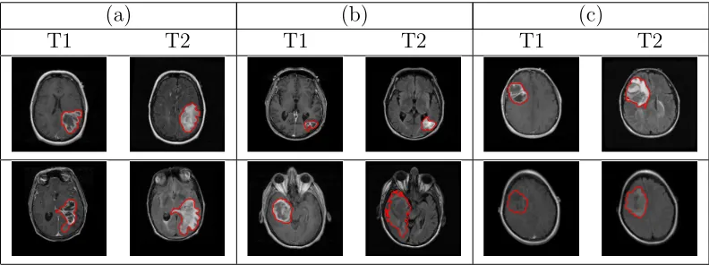
(a) (b) (c)
[image:8.612.107.503.67.215.2]T1 T2 T1 T2 T1 T2
Figure 2: Examples of manually segmented tumor contours overlaid on the T1 and T2 images for patients with (a) short (<1 month), (b) medium (≈15 months) and (c) long (>50 months) survival. Each row represents a different tumor.
We adopt the shape definition of Srivastava et al. (2011) that is particularly attractive in the current context (see Joshi et al. (2007), Srivastava et al. (2011) and Kurtek et al. (2012) for details). While describing the tools, we concurrently illustrate their usage on the GBM dataset. To get an idea of this problem’s complexity, we display a few examples of tumor contours overlaid on the corresponding T1 and T2 MRI slices in Figure 2 (each row represents a different tumor). The tumor shapes are heterogeneous, and at first glance it is difficult to ascertain any relationship between tumor shapes and survival times. To obtain insight into possible relationships between tumor shapes and outcomes, more sophisticated approaches are required. Throughout this section, we use the word metric to refer to a Riemannian metric (i.e., an inner product in tangent spaces), and distance to refer to the measure of differences between objects.
3.1 Representation of tumor shape and elastic metric
The tumor shapes should be invariant to translation and rotation. Scaling might be con-sidered important, and can easily be incorporated into our framework. Denote a parame-terized, planar, closed curve representing the outline of a tumor by a functionβ :S1 →
R2.
circle domain S1, instead of an interval. There are several possibilities for representing β
for the purpose of shape analysis. One can simply use the x and y coordinate functions of β; another possibility is to parameterizeβ using the arc length and compute the angle
˙
β = dβdt makes with the x-axis (here, t is the curve parameter) (Klassen and Srivastava, 2006). For an overview of the different possible representations, and associated properties of shape spaces, see Bauer et al. (2014).
The choice of a metric on the tumor shape space is vital for comparing two shapes. Unlike typical problems in shape analysis, there is no template shape available while con-sidering tumors. In this context, it is imperative that the metric capture all possible deformations that match one tumor shape to another. One candidate metric is the elastic metric, defined as follows. Supposep(t) = |β˙(t)|is the speed function andθ(t) = ˙β/|β˙(t)|is the angle function. Consider two tangent vectors (small perturbations) (δpi, δθi), i= 1,2
in the tangent space of (p, θ). The elastic metric (Mio et al., 2007) is defined as:
h(δp1, δθ1),(δp2, δθ2)i(p,θ) =a
Z
S1
δp1(t)δp2(t)1/p(t)dt+b
Z
S1
hδθ1(t), δθ2(t)ip(t)dt, (1)
for constants a, b > 0. The first term in Equation (1) measures variations in the speed function (i.e., how fast the tumor outline is traversed), while the second term measures the variation in the direction of the unit tangent vectors via the standard Euclidean inner product betweenδθ1 andδθ2 (denoted byh·,·i);aandb provide the relative weights for the
two terms. In other words, the first term captures the amount of stretching and the second term captures the amount of bending required to deform one tumor shape into another. Both terms are needed to generate natural deformations between tumor shapes. However, choosing a and b is hard and problem-dependent.
in many different ways, but it’s shape remains unchanged. A common approach in the shape analysis literature is to normalize curve parameterizations to arc length to ensure that traversal along the curve is at unit speed. Under this scenario, only bending deforma-tions are allowed, which often results in suboptimal point correspondences across shapes (Mio et al., 2007). We describe how it is possible to not only efficiently employ the elastic metric, but also ensure that the resulting geodesic distance is invariant to the choice of parameterization. Unless otherwise stated, all curves are parameterized via arc length.
3.1.1 Square-root velocity function
Let Γ = {γ : S1 →
S1|γ is an orientation-preserving diffeomorphism} be the group of
re-parameterization functions, and orientation imply clockwise or counter-clockwise traversal of the contour (i.e., γ is an invertible function that maps the unit circle to itself and preserves direction). The re-parameterization of a tumor curve β, termed the action of Γ on the space of curves, is given by composition: (β, γ) =β◦γ. The chief issue with using the popular L2 metric is that the distance between two tumor contours β1 and β2 is not
preserved under the action of Γ: kβ1−β2k 6=kβ1◦γ−β2◦γkfor a generalγ ∈Γ. In other
words, the action of Γ on the space of tumor curves is not isometric, which means that a comparison of two tumor shapes depends on their parameterizations.
A proposed solution (Joshi et al., 2007; Srivastava et al., 2011; Kurtek et al., 2012) is to use a different representation of curves called the square-root velocity function (SRVF), given by q(t) = √β˙(t)
|β˙(t)|, where | · | is the standard Euclidean norm in R
2. This
representa-tion is convenient because it is automatically translarepresenta-tion invariant. Conversely, β can be reconstructed from q up to a translation. If a tumor curve β is re-parameterized to β◦γ, then its SRVF changes from q to (q, γ) = (q◦γ)√γ˙.
The main reasons for using the SRVF for tumor shape analysis are: (1) the complicated but desirable elastic metric reduces to the standardL2metric witha= 1/4 andb= 1,
for all γ ∈ Γ, allowing for parameterization invariant analysis of tumor shapes. If in-variance to scale is required, each tumor shape can be re-scaled to unit length. After re-scaling, kqk2 =R
S1|q(t)|
2dt =R
S1| ˙
β(t)|dt = 1, i.e., the representation space of all SRVFs is a Hilbert sphere. For tumor shapes, the size of the tumor is often important, and the variability in tumor shape due to scale differences is considered to be important as well. In the GBM data example, we decouple tumor shape and size and consider them individually as covariates in the survival models. For a closed curve, which characterizes the tumor con-tours we are studying, the corresponding SRVF satisfies the additional closure condition
R
S1q(t)|q(t)|dt = 0. Thus, the space of all unit length, planar, closed tumor curves, repre-sented by their SRVFs, is given byC =
n
q:S1 →R2|R
S1|q(t)|
2dt = 1, R
S1q(t)|q(t)|dt = 0
o
, and is called the pre-shape space.
3.1.2 Geodesic paths and distances in the elastic shape space
In the absence of a template tumor shape, it is critical to visualize deformations or changes in tumor shape. The choice of the elastic metric and the SRVF of two tumor shapes make it possible to compute natural geodesic paths and distances between them; as a consequence,
we can visually examine the meaningful deformations of one tumor shape that transforms it
into the other by traversing the geodesic path. This is potentially useful to radiologists for assessing possible changes in tumor morphology, thereby facilitating targeted interventions.
Pre-shape space C with parameterization and rotation variability: The pre-shape spaceC is a nonlinear submanifold of the Hilbert sphere due to the closure condition. It becomes a Riemannian manifold with the standard L2 metric, hhv1, v2ii =
R
S1hv1(t), v2(t)idt, where
v1, v2 ∈Tq(C) (i.e., v1 and v2 are elements of the tangent space to C at q; they are often
referred to as shooting vectors) and the inner product in the integrand is the standard Euclidean inner product in R2. The task of computing geodesic paths between any two
elementsq1, q2 ∈ C is accomplished numerically, using an algorithm called path
by Srivastava et al. (2011). This algorithm initializes a path in C connectingq1 and q2, and
iteratively ‘straightens’ it until it becomes a geodesic. The geodesic distancedCis then
sim-ply the length of the geodesic path. The issue with dC is that it contains contributions from
two nuisance sources of variation. The distance between two tumor outlines is non-zero when they are within (1) a rotation and/or (2) a re-parameterization of each other.
Shape space S accounting for parameterization and rotation variability: To remedy the is-sues with the pre-shape geodesic distance dC between two tumor shapes, it needs to be
computed while accounting for all possible (1) rotations and (2) re-parameterizations of one tumor shape to optimally register it to the other. This is achieved as follows.
Let SO(2) be the set of 2× 2 rotation matrices (special orthogonal group). For a tumor contour β and a rotation O ∈ SO(2), the SRVF of the rotated curve Oβ is given by Oq. Thus, in order to unify all elements in C that denote the same tumor shape, we define equivalence classes of the type [q] = {O(q◦γ)√γ˙|O ∈ SO(2), γ ∈ Γ}. Each such equivalence class [q] is associated with a unique tumor shape and vice versa. The set of all equivalence classes is called theshape spaceS and is the quotient spaceC/(SO(2)×Γ). The distance dC can be used to define a distance between tumor shapes on S according to
dS([q1],[q2]) = inf
O∈SO(2), γ∈ΓdC(q1,(Oq2, γ)). (2)
The geodesic distance dS is now the elastic distance on the space of tumor shapes and is
invariant to rotation and re-parameterization; as a consequence, all possible deformations pertaining to stretching and bending of tumor shapes are captured. Moreover,dS is bounded
above by π/2, thereby offering a natural scale for comparing tumor shapes. In practice, the minimization in the definition of dS is performed by sampling each curve with a large
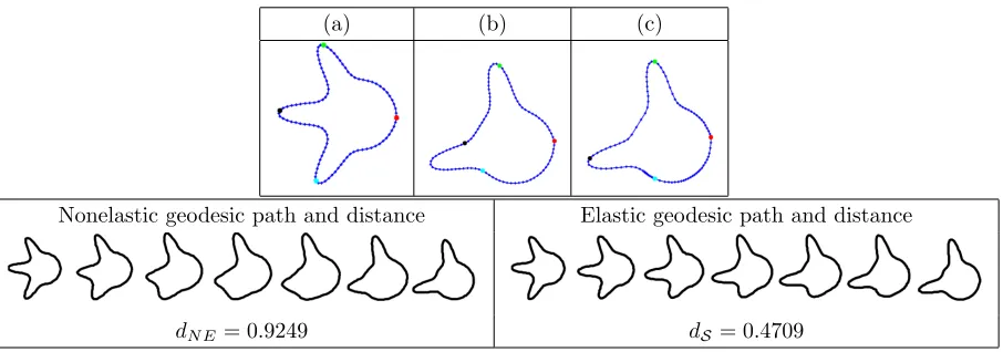
(a) (b) (c)
Nonelastic geodesic path and distance Elastic geodesic path and distance
[image:13.612.82.535.65.224.2]dN E= 0.9249 dS = 0.4709
Figure 3: Comparison of two simulated tumor shapes. (a) Curve with three protruding peaks. (b) Curve with two protruding peaks before re-parameterization (uniform spacing of points). (c) Same as (b) after re-parameterization (optimal non-uniform spacing of points). We show four colored points of correspondence for improved visualization. The resulting geodesic paths are sampled uniformly using seven points (NE=nonelastic).
Illustrative examples: We present multiple simulated and real data examples comparing nonelastic geodesic paths and distances (we only optimize over rotations and the seed placement but not the full re-parameterization group) to the proposed elastic versions computed in the shape space. The points along the geodesic path between two tumor shapes should be viewed as the possible deformations transforming one tumor shape into the other. Since, in contrast to elastic shape analysis, the nonelastic framework does not allow stretching and compression deformations, we observe some unnatural shapes appearing along the geodesic paths in that case.
(a) (b) (c) (d) (e) (f)
Nonelastic geodesic path and distance Nonelastic geodesic path and distance
dN E = 0.9946 dN E = 0.5324
Elastic Geodesic path and distance Elastic geodesic path and distance
[image:14.612.74.534.67.271.2]dS = 0.5324 dS = 0.4242
Figure 4: Left: Comparison of T1 tumor shapes for a patient with survival time of 14.3 months and for a patient with survival time of 29.2 months. Right: Comparison of T1 tumor shapes for a patient with a short survival time (8.8 months) and for a patient with a long survival time (48.6 months). (a)&(d) Curve representing first tumor. (b)&(e) Curve representing second tumor before re-parameterization (uniform spacing of points). (c)&(f) Same as (b)&(e) after re-parameterization (optimal non-uniform spacing of points). We show four colored points of correspondence for improved visualization. The resulting geodesic paths are sampled uniformly using seven points (NE=nonelastic).
nonelastic geodesic deformation between these two shapes, where two of the peaks on the first shape are distorted to form the second peak on the second shape; the resulting distance is dN E = 0.9249. Under the elastic framework on the shape space S, the optimal
re-parameterization is able to match the first two peaks across the two curves very well (green and black points). Of course, there is no counterpart to the third peak on the second curve (cyan point). This results in a natural deformation where the two matched peaks are preserved along the geodesic path while the third one simply grows; the resulting distance isdS = 0.4709 (nearly a 50% decrease). We hypothesize that improvements such as the one
in this simulated example are extremely important in capturing natural variability in GBM tumor shapes. Upon visual inspection, the observed tumor contours have many geometric structures such as the peaks in this example. This motivates the use of the elastic shape analysis framework for studying GBM tumors.
(a) (b) (c) (d) (e) (f)
Nonelastic geodesic path and distance Nonelastic geodesic path and distance
dN E = 1.1209 dN E = 1.0113
Elastic Geodesic path and distance Elastic geodesic path and distance
[image:15.612.74.534.68.260.2]dS = 0.6024 dS = 0.5346
Figure 5: Left: Comparison of T2 tumor shapes for a patient with survival time of 2.69 months and for a patient with survival time of 13.3 months. Right: Comparison of T2 tumor shapes for a patient with survival time of 6.14 months and for a patient with survival time of 0.72 months. Panels (a)-(f) are the same as in Figure 4.
survival times; Figure 4 presents two examples for the T1 modality, whereas Figure 5 considers the T2 modality. In all examples, we have marked four corresponding points in red, green, black and cyan, and show the stretching and compression of points along the tumor curve due to optimization over Γ. The benefit of using the elastic framework becomes apparent when computing and visualizing geodesic paths between the tumor shapes: the points along the path represent tumor shapes that are elastically deformed in a natural way and preserve important shape features of the tumors. Indeed, when we allow non-uniform spacing of points along the curves, the geodesic deformation is improved due to an improved matching of geometric features across the tumor shapes. For example, for the T1 example in the left panel of Figure 4, the deformations along the geodesic path defined through the distancedS are natural in the following sense: the highly concave geometric feature of both
the nonelastic (dN E) and elastic (dS) frameworks. Improvements of this form are also even
more drastic when one considers statistical modeling of such tumor shapes. The presented examples thus support our proposal for the use of elastic shape analysis of GBM tumors for association with patient survival and genomic variables.
3.2 Statistical summaries of tumor shapes
Hereafter, our analyses focus on the shape space S and the distance dS. However, we
illustrate the resulting differences in the statistical summaries under nonelastic and elastic shape analysis. We define and illustrate computations of a mean tumor shape and co-variance of a sample of tumor shapes, both defined with respect to dS. Consequently, we
demonstrate how sPCA can be applied to explore and visualize the directions of variation in tumor shape based on patient-level information. Identifying such directions can be useful in understanding the most likely deformations of the tumor shapes, and can be potentially used to monitor the disease and for targeted therapeutic interventions.
3.2.1 Mean and covariance
Under the SRVF framework, the shape space S is a (quotient space of a) nonlinear sub-manifold of the Hilbert sphere, which is equipped with a Riemannian structure under the L2 metric. We first introduce some notation. Let q
1, q2 ∈ C be the SRVFs of two
tumor pre-shapes and v ∈ Tq1(C). Then, the maps q2 7→ v = exp
−1
q1 (q2) ∈ Tq1(C) and
v 7→ q2 = expq1(v) ∈ C are the exponential and inverse exponential maps, respectively. These are not available analytically for the pre-shape space of closed curves; algorithms for computing these quantities are similar to the technique for finding geodesics (Srivastava et al., 2011).
corresponding SRVFs. Then, the Karcher (Frechet) mean tumor shape is defined as
[¯q] = argmin
[q]∈S n
X
i=1
dS([q],[qi])2. (3)
A gradient-based approach for finding this mean is provided in Le (2001) and Dryden and Mardia (1998), and is omitted here for brevity. The Karcher mean is actually an entire equivalence class of curves. For the remainder of our analysis, we select one element of this class ¯q ∈ [¯q]. One could also use the more robust geometric median as an alternative representative shape (Fletcher et al., 2009; Kurtek et al., 2013); for simplicity, we do not consider this case in the current work.
The general computation of the covariance around the estimated shape mean is as follows. Let vi = exp−q¯1(qi∗),i= 1, . . . , n denote the shooting vectors from the mean shape
to each of the shapes in the given data. This first involves an optimal rotation O∗ and optimal re-parameterization γ∗ of each qi, resulting inqi∗ = (O
∗q
i, γ∗), to register it to the
mean shape ¯q. Then, the covariance kernel can be defined as a function Kq :S1×S1 →R
given by Kq(ω, τ) = (1/(n−1))
Pn
i=1hhvi(ω), vi(τ)ii. In practice, since the curves have to
be sampled with a finite number of points, say m, the resulting covariance matrices are finite-dimensional. Often, the observation size n is much less thanm and, consequently, n
controls the degree of variability in the stochastic model.
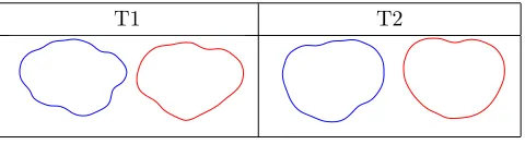
T1 T2
Figure 6: Comparison of elastic (blue) and nonelastic (red) shape averages of T1 and T2 tumors.
T1 elastic T1 nonelastic
[image:18.612.114.499.175.280.2]T2 elastic T2 nonelastic
Figure 7: Comparison of elastic and nonelastic principal directions of variation for T1 and T2 tumor shapes. In each example, we display the path within two standard deviations of the mean (red).
3.2.2 Shape-based principal component analysis
We explore dominant directions of variation in a sample of tumor shapes with an efficient basis for T[¯q](S) using traditional PCA (also referred to as tangent PCA). While one could
also use the Principal Geodesic Analysis developed in Fletcher et al. (2003) for the same purpose, we choose the simpler tangent PCA method for data analysis in this work. Let
V ∈R2m×n be the observed tangent data matrix with nobservations and m sample points
inR2 on each tangent, i.e., each column of V isv
i = exp−q¯1(qi∗),i= 1, . . . , n, stacked into a
long vector. Let K ∈R2m×2m be the resulting covariance matrix and let K =UΣUT be its
SVD. The submatrix formed by the first rcolumns ofU, called ˜U, spans ther-dimensional principal subspace of the observed shapes and provides the observations of the principal coefficients asC= ˜UTV ∈Rr×n. Thus, each original tumor shape can be represented using
a finite set of principal coefficients acting as Euclidean coordinates. These coefficients can then be used in a survival model for prediction as shown later.
an effective and common qualitative assessment (Shen et al., 2009; Epifanio and Ventura-Campos, 2014). For each case, we compare the elastic and nonelastic methods. The elastic principal paths capture more geometric features and are better at representing the overall variability in the tumor shapes. We compute the overall variance for each sPCA model as 7.86 (elastic) and 12.74 (nonelastic) for T1 tumors, and 13.43 (elastic) and 27.68 (nonelastic) for T2 tumors. The elastic models are more compact and provide a more efficient Euclidean representation of the tumor shapes in terms of the principal coefficients. Note that due to a high level of heterogeneity of the tumor shapes, over 30 elastic sPCA components are needed to explain more than 95% of the variance. In Section 2 of the Supplementary Material, we additionally show that the elastic approach provides more natural results in the context of sPCA-based shape modeling and reconstruction.
4
Shape-based clustering, testing and survival analysis in GBM
The elastic framework for analyzing tumor shapes allows one to perform a variety of estima-tion and inferential statistical tasks. In particular, sPCA of tumors provides the possibility of devising methods based on principal coefficients, which can be profitably viewed as Eu-clidean features or summaries of the tumor shape for inclusion in regression models. Using a dataset of MRIs of GBM brain tumors, we applied clustering, two-sample testing, and survival modeling to illustrate the advantages associated with the elastic representation of tumor shapes and the related geometric framework in the context of assessing patient sur-vival and association with genomic/clinical variables. Note that from here on, we perform statistical analysis via the elastic framework only.
4.1 Clustering of GBM tumor shapes
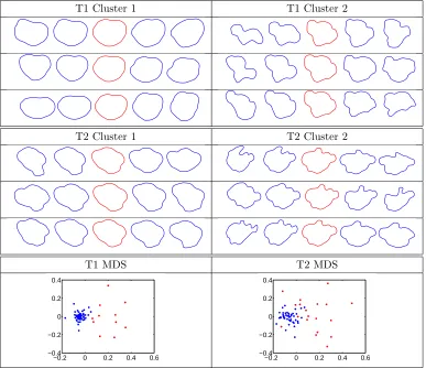
T1 Cluster 1 T1 Cluster 2
T2 Cluster 1 T2 Cluster 2
T1 MDS T2 MDS
−0.2 0 0.2 0.4 0.6 −0.4
−0.2 0 0.2 0.4
−0.2 0 0.2 0.4 0.6 −0.4
[image:20.612.113.500.68.402.2]−0.2 0 0.2 0.4
Figure 8: Cluster-wise principal directions of variation for T1 and T2 tumor shapes. In each example, we display the path within two standard deviations of the mean (red). Bottom: Multidimensional scaling plots of the T1 and T2 tumor shape data (cluster 1=blue, cluster 2=red).
and then used complete linkage to separate the shapes into two clusters for each modality (motivated by short vs. long survival and supported by cluster visualization; see bottom panel of Figure 8). To better visualize the variability in each cluster, we performed cluster-wise sPCA and plotted the three principal directions of variation in each cluster for the T1 and T2 modalities in Figure 8. We also report the cumulative variance in each cluster in Table 1. For both modalities, the variance in cluster 1 is much smaller than the variance in cluster 2. This can also be seen in the principal directions of variation; the shapes shown along cluster 1 directions (including the mean shape) are smoother and more circular.
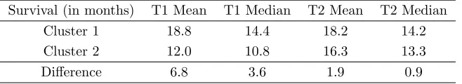
Cumulative Variance T1 T2 Cluster 1 5.51 10.23 Cluster 2 14.74 17.95
Table 1: Cumulative variance of the cluster-wise sPCA models for the T1 and T2 tumor data. Survival (in months) T1 Mean T1 Median T2 Mean T2 Median
Cluster 1 18.8 14.4 18.2 14.2
Cluster 2 12.0 10.8 16.3 13.3
Difference 6.8 3.6 1.9 0.9
Table 2: Summaries of cluster-wise survival for the T1 and T2 tumor data.
the separability of the clusters is very good for both modalities suggesting that the choice of two clusters is appropriate in this setting. In Table 2, we provide the mean and median survival times associated with the clusters, computed using tumor shape data in each modality. First, the T1 modality provides better discrimination between survival times than the T2 modality. Furthermore, for both modalities, we see that the mean and median survival times are higher in cluster 1, which contains much lower cumulative variance. This suggests that cluster 1 is more homogeneous, which is associated with longer survival times; cluster 2 is more heterogeneous and is associated with shorter survival times. This can also be attributed to the general morphological structure of tumors in the two clusters. The tumors in cluster 1 are often smoother and more circular than those in cluster 2, which are more irregular. It is this irregularity that is indicative of a more severe and infiltrative tumor with blurred margins, and as a result, shorter survival times. Note that the mean difference in survival times between cluster 1 and cluster 2 computed using T1 tumor shapes is 6.8 months, which is large compared to the 12 month median survival time in GBM.
4.1.1 Cluster validation via enrichment
[image:21.612.143.472.157.217.2]T1 T2
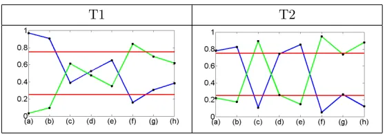
Figure 9: Enrichment plots for the T1 and T2 modalities: (a) classical; (b) mesenchymal; (c) proneural; (d) EGFR; (e) MDM4; (f) PDGFRA; (g) PIK3CA; (h) PTEN. The red lines indicate the 0.75 and 0.25 cutoffs for ‘high’ enrichment in cluster 1 (blue) and cluster 2 (green), respectively.
want to compare the relative occurrence of a specific dichotomous covariate (with label 0 for no occurrence and 1 for occurrence) across the two clusters. To develop a Bayesian model for this purpose, letθ1 ∈[0,1] (θ2 ∈[0,1]) denote the true proportion of 1s (0s) in cluster 1; let
y1(y2) denote the observed number of 1s (0s) in cluster 1. Then,y1 ∼Binomial(n1, θ1) and
y2 ∼Binomial(n2, θ2), wheren1 is the total number of 1s andn2 is the total number of 0s.
Consider aBeta(1,1) prior on the true proportionsθ1 andθ2. Since the Beta distribution is
conjugate for the Binomial, the posterior distribution is of the same family as the prior; the resulting posterior distributions forθ1 andθ2 are given byπθ1(θ1|y1, n1)∼Beta(y1+ 1, n1−
y1+1) andπθ2(θ2|y2, n2)∼Beta(y2+1, n2−y2+1). We generate a large number of samples from the two posteriorsπθ1 andπθ2, and approximate the true probabilityP(θ1 > θ2) using Monte Carlo. We refer to this approximate quantity as the enrichment probability. The intuition behind this approach is as follows. If the computed clusters are not associated with the dichotomous covariate of interest, the resulting posteriors for θ1 and θ2 should be
very similar. This in turn results in a Monte Carlo estimate of P(θ1 > θ2) close to 0.5,
or no enrichment. On the other hand, when the two posteriors are drastically different, the Monte Carlo estimate of P(θ1 > θ2) would be either very close to 1 (if y1 is much
larger than y2) or 0 (if y1 is much smaller than y2). These two scenarios constitute high
enrichment of the covariate in one of the two computed clusters (a given covariate can be enriched in only one cluster at a time).
as a line plot with high and low cutoffs in the form of horizontal lines at 0.75 and 0.25. We note the following trends from the enrichment plots. The classical and mesenchymal tumor subtypes are enriched in cluster 1 for both modalities. The proneural tumor subtype is enriched in cluster 2 for the T2 modality. Interestingly, the mesenchymal subtype, a very aggressive form of GBM, was enriched in the cluster with higher survival. However, upon closer examination, there was an equal number of mesenchymal and nonmesenchymal subtypes in cluster 1 for both modalities (the enrichment probability was mostly driven by the arrangement in cluster 2). Furthermore, the patients in cluster 1 with the mesenchymal subtype had lower survival than their nonmesenchymal counterparts (by ∼1.5 months).
The enrichment plots for both imaging modalities display results consistent with some of the well-characterized genomic signatures in GBM. We note the following strong asso-ciations between tumor subtypes and driver gene mutations that have also been found in other studies (McNamara et al., 2013; Verhaak et al., 2010): (1) proneural subtype and PDGFRA mutation (in T2), and (2) classical and mesenchymal subtypes and EGFR mu-tation (in T2). EGFR mumu-tation is a common molecular signature of GBM. It promotes proliferation of the tumor, which is associated with classical and mesenchymal subtypes (Fischer and Aldape, 2010). PDGFRA also plays an important role in cell proliferation and migration, and angiogenesis. Unlike EGFR, this gene was found to be mutated in high amounts in the proneural subtype of GBM tumors only (Verhaak et al., 2010).
4.2 Permutation test for difference in tumor shape means
The distance dS between two tumor shapes opens up the possibility of a distance-based
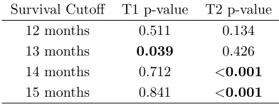
Survival Cutoff T1 p-value T2 p-value 12 months 0.511 0.134 13 months 0.039 0.426 14 months 0.712 <0.001
[image:24.612.206.402.69.142.2]15 months 0.841 <0.001
Table 3: Permutation test results for T1 and T2 tumor shapes.
the case of landmark-based shape analysis (Dryden and Mardia, 1998) can be constructed under no assumptions on the distributions of the two groups. For each cutoff, we calculate the test statistic, which is the shape distance dS between the Karcher mean estimates for
the two groups based on the given data. The distribution of this test statistic under the null hypothesis is not easily determined. Thus, we employ a permutation test by combining shapes from both samples (survival labels are exchangeable under the null hypothesis). We use 1000 random permutations of the labels to generate the distribution of the test statistic. The resulting p-values for the T1 and T2 modalities, and all of the cutoffs, are presented in Table 3. Based on our test statistic, there is a significant difference between T1 mean tumor shapes at the 0.05 level only at the 13-month cutoff. For the T2 tumor shapes, there is a highly significant shape mean difference for the 14- and 15-month cutoffs. The results clearly depend on the choice of the cutoff; nevertheless, this result provides support for our hypothesis that tumor shape features can be useful in survival analysis in GBM studies. We only use the mean shape information in this hypothesis test, although we expect that the covariance information is also useful. We demonstrate how that can be achieved using a principal coefficient representation of tumor shapes in subsequent survival modeling.
4.3 Survival model adjusted for tumor shape
in the presence of genetic and clinical covariates, using the geometry-based elastic shape method. Upon performing sPCA in the shape spaceS, each tumor shape is represented in the principal directions of variation basis via its principal coefficients, which can be used as predictors in a survival model. Geodesic paths constructed using principal shooting vectors allow for the possibility of traversing the principal directions of shape variation and monitoring changes in the shape of a tumor. It is customary to choose a handful of principal directions that explain most of the shape variability; however, since S is infinite-dimensional, and it is unclear how one can interpret the directions in the context of tumor shapes, we propose to use all available directions to capture maximal information from the data. Indeed, it may very well be that a direction corresponding to a small (in magnitude) eigenvalue represents a physiologically important tumor shape deformation. In order to incorporate all information from the images, we perform separate sPCA on tumors ob-tained fromboth T1 and T2 MRIs, and collate the principal coefficients from each imaging modality. Employing all available shape principal coefficients translates to a large number of imaging-based shape predictors in a potential survival model necessitating dimension reduction through variable selection.
To assess whether incorporating imaging covariates, through principal tumor shape coefficients, improves discriminatory power of the survival model, we compare three nested models: (1) M1, a model with a set of clinical covariates C; (2)M2, a model with clinical and a set of genetic covariates G; and (3) M3, a model with clinical, genetic and a set of imaging covariatesI in the form of shape principal coefficients; note thatM1⊂M2⊂M3 where A⊂B denotes that model A is nested within model B.
and M3 := Cox model with C ∪G ∪ I. Importantly, model M3, with a large number of tumor shape principal coefficients as predictors (62 each for T1 and T2), is fitted to the data by penalizing the negative log-likelihood using a lasso penalty. Furthermore, we use leave-one-out cross-validation to determine the value of the penalty parameter. Specifically, if η is the vector of coefficients, then M3 is fit by solving the optimization problem minη
h
- log-partial likelihood of M3i+λ|η|1, where |η|1 is the L1 norm of η. We
use the R packageglmnet by Friedman et al. (2011) for our implementation of modelM3 with leave-one-out cross-validation. The setI is then redefined to contain only the principal coefficients with non-zero regression coefficients obtained from this lasso regression.
4.3.1 Significant directions of shape variation and other results
Results from fitting the three Cox models are given in Table 4. Gutman et al. (2013) found significant association between the clinical covariateKPSand survival time, adjusting for the presence of other numerical radiological summaries; this agrees with our results for all three models. Although the KPSscore is measured on a scale of 0-100, the only distinct values in our dataset were 60, 80 and 100 along with missing values for 12 patients. As a measure of the ability to perform activities of daily living, theKPSscores only influence the survival time indirectly, and in this dataset, they complement the influence of the tumor shape principal coefficients. Since tumor volume was recorded for each patient from T1 and T2 images, we considered the shapes of tumor outlines rather than shapes and sizes. The size of the tumor was included in the model as a separate covariate through the tumor volume. It is known that tumors with EGFR mutations are larger than tumors with other mutations (Hatanpaa et al., 2010). In our analyses,EGFRand tumor volumes from both T1 and T2 images were not found to significantly correlate with survival time in the presence of tumor shape information. This finding is at odds with that of Gutman et al. (2013) where lesion size was used. It is known that older patients with GBM show high EGFR
amplification. However, the variable EGFR informs us only if a mutation has occurred, not amplification. The age of a patient diagnosed with GBM is known to influence the survival time (Weller and Wick, 2011). Older age is typically used as a surrogate marker for change in the biology of GBM. The mean age in our dataset was 56.33 years; the variable Age
appeared to have significant correlation with survival time in all three models, and the inclusion of tumor shape information did not alter that.
Model Predictors C-index 1 C-index 2
Significant at 0.05 (Harrell et al., 1982) (G¨omen and Heller, 2005)
M1 Age, KPS 0.641 0.652
Clinical
M2 Age, KPS 0.722 0.728
Clinical+Genetic DDIT3, PIKC3A
[image:28.612.81.531.68.185.2]M3 Age, KPS, DDIT3 0.859 0.841 Clinical+Genetic+Imaging 11 PC shape coefs
Table 4: Results from fitting Cox models M1,M2 and M3. Predictors significant at the 5% level are tabulated, and the two concordance indices are reported.
the C-indices for M2 andM1. This indicates a clear benefit in incorporating tumor shape predictors in the form of principal coefficients into a survival model in order to obtain good discriminatory power. The Kaplan–Meier estimates of the survival functions for the three models, along with a description, are provided in Section 3 of the Supplementary Material. In summary, amongst the driver genes known to be significant in GBM studies, only
DDIT3 appears to have a significant correlation with the survival time of a patient when
adjusted for the effect of tumor shape. Mutation of the driver gene DDIT3 appears to be associated with low survival probability (see Figure 6 in the Supplementary Material); it is known to indirectly regulate the glioma pathway through unregulated genes. Our analyses indicate that the shape of the tumor captures sufficient information about the individual relationships between each of the driver genes and survival time. A deeper study of the relationships between the shape of the tumor and driver genes is well worth exploring.
5
Discussion and future work
using Procrustes averaging were used to study schizophrenia by DeQuardo et al. (1996). However, landmark and descriptor-based methods are not directly applicable to oncology due to multiple issues mentioned in this paper. In this work, we provide a comprehensive, Riemannian geometric solution to this problem that provides tools for various statistical analyses of tumor shapes. The benefits of this framework are clear: (1) it provides an elastic metric to measure interpretable shape deformations, (2) it defines a formal mathematical and statistical framework, and (3) it provides tools for shape alignment, comparison, sum-marization, clustering, classification, hypothesis testing and other tasks. We demonstrate these benefits through a detailed study of tumor shapes in the context of GBM. The pro-posed method can be readily extended to any cancer and/or other imaging modalities with similar data characteristics and scientific questions.
The focus of this article is on 2D tumor shapes obtained from the segmented tumor of a single axial slice of the brain with largest tumor area. The influence of the location and anisotropic nature of the white matter tracts on the shape of the tumor can be better assessed with 3D shape analysis, which is currently in progress. The geometric framework presented in this paper allows for the extension to 3D shapes (square-root normal fields (Jermyn et al., 2012)), which would allow one to capture the full elastic shape of the tumor. However, studying parameterized surfaces in this context is difficult due to the large shape heterogeneity of the tumors. Except for the work of Goldberg-Zimring et al. (2005) who used spherical harmonic functions to model the 3D shape of a tumor (akin to nonelastic analysis of tumor shapes), there is a lack of progress in this direction.
One way to view the proposed survival model is within the context offered by regres-sion with functional predictors. The parametric closed curve representing a tumor shape predictor can be viewed as an element of the pre-shape space C, which is a submanifold of L2(
S1) and not a vector space. Current approaches with functional predictors using
The geometric framework used in this article enables us to perform PCA on the space of tumor shapes under a Riemannian metric. The physiological interpretation of the prin-cipal directions, however, is unclear and much work remains to be done in this direction. Construction of a set of basis functions for the tangent space of a tumor shape that cap-tures the biologically relevant deformations of the shape would be particularly useful; this requires significant input from clinicians in the form of prior shape information. The defor-mations observed in the tumor shape as we move away from the mean along the direction of decreased survival are striking; the shape appears to become more spiculated, which is consistent with the heuristic understanding of the seriousness of an irregularly shaped tumor. The visualization afforded within our framework, in our opinion, can profitably be used by neuroradiologists for initial non-invasive diagnoses. An alternative approach would be to use sparse PCA methods to model the variability in tumor shapes, which has recently proven useful in generating results that are clinically interpretable (Sj¨ostrand et al., 2007). Applying the survival model M3 to the GBM dataset, we uncover several potentially interesting relationships between the shape of the tumor (expressed through the principal coefficients) and driver genes. This merits further consideration, and the implementation of our methods on other GBM datasets would offer more insight. Biological validation of the correlations between the two can significantly impact targeted personalized treatment strategies for GBM patients. Importantly, prognostic biomarkers of the transition time from a low-grade glioma to a malignant one can be determined.
supported by NIH grants R01-CA194391 and R01160736, NSF grant 1463233, and CCSG from NIH/NCI (P30-CA016672).
References
Affronti, M. L., C. R. Heery, J. E. Herndon, J. N. Rich, D. A. Reardon, A. Desjardins, et al. (2009). Overall survival of newly diagnosed glioblastoma patients receiving carmustine wafers followed by radiation and concurrent temozolomide plus rotational multiagent chemotherapy. Cancer 115(1), 3501–3511.
Bauer, M., M. Bruveris, and P. W. Michor (2014). Overview of the geometries of shape spaces and diffeomorphism groups.Journal of Mathematical Imaging and Vision 50(1-2), 60–97.
Cox, D. R. (1972). Regression models and life-tables. Journal of Royal Statistical Society, Series B 34(1), 187–220.
Crooks, V., S. Waller, T. Smith, and T. J. Hahn (1991). The use of Karnofsky Performance Scale in determining outcomes and risk in geriatric outpatients. Journal of Gerontol-ogy 46(4), 139–144.
De Sousa, F. E. M., L. Vermeulen, E. Fessler, and J. P. Medema (2013). Cancer hetero-geneity - a multifaceted view. EMBO reports 14(8), 686–695.
DeQuardo, J. R., F. L. Bookstein, W. D. K. Green, J. A. Grunberg, and R. Tandon (1996). Spatial relationships of neuroanatomic landmarks in schizophrenia. Psychiatry research: Neuroimaging 67(1), 311–318.
Dryden, I. L. and K. V. Mardia (1998). Statistical Shape Analysis. John Wiley & Son.
Fischer, I. and K. Aldape (2010). Molecular tools: Biology, prognosis, and therapeutic triage. Neuroimaging Clinics of North America 20(3), 273 – 282.
Fletcher, P. T., C. Lu, and S. C. Joshi (2003). Statistics of shape via principal geodesic analysis on Lie groups. InIEEE CVPR, pp. 95–101.
Fletcher, P. T., S. Venkatasubramanian, and S. C. Joshi (2009). The geometric median on Riemannian manifolds with application to robust atlas estimation. NeuroImage 45(1), S143–S152.
Frattini, V., V. Trifonov, J. M. Chan, A. Castano, M. Lia, F. Abate, et al. (2013). The inte-grated landscape of driver genomic alterations in glioblastoma. Nature Genetics 45(10), 1141–1149.
Friedman, J., T. Hastie, and R. Tibshirani (2011). Regularization paths for Cox’s pro-portional hazards model via coordinate descent. Journal of Statistical Software 39(5), 1–13.
Goldberg-Zimring, D., A. Achiron, S. Miron, M. Faibel, and H. Azhari (1998). Automated detection and characterization of multiple sclerosis lesions in brain MR images. Magnetic Resonance Imaging 16(1), 311–318.
Goldberg-Zimring, D., I.-F. Talos, J. G. Bhagwat, S. J. Haker, P. M. Black, and K. H. Zou (2005). Statistical validation of brain tumor shape approximation via spherical harmonics for image-guided neurosurgery. Academic Radiology 12(1), 459–466.
Goldsmith, J., L. Huang, and C. M. Crainiceanu (2013). Smooth scalar-on-image regres-sion via spatial Bayesian variable selection. Journal of Computational and Graphical Statistics 23(1), 46–64.
Gutman, D. A., L. A. D. Cooper, S. N. Hwang, C. A. Holder, J. Gao, T. D. Aurora, et al. (2013). MR imaging predictors of molecular profile and survival. Radiology 267(2), 560–569.
Harrell, F. E., R. Califf, D. Pryor, K. Lee, and R. Rosati (1982). Evaluating the yield of medical tests. Journal of the American Statistical Association 247(1), 2543–2546.
Harrell, F. E., R. Califf, D. Pryor, and R. Rosati (1984). Regression modelling strategies for improved prognostic prediction. Statistics in Medicine 3(1), 143–152.
Hatanpaa, K. J., S. Burma, D. Zhao, and A. A. Habib (2010). Epidermal growth factor receptor in glioma: Signal transduction, neuropathology, imaging, and radioresistance.
Neoplasia 12, 675–684.
Jermyn, I. H., S. Kurtek, E. Klassen, and A. Srivastava (2012). Elastic shape matching of parameterized surfaces using square root normal fields. In ECCV, pp. 804–817.
Joshi, S. H., E. Klassen, A. Srivastava, and I. H. Jermyn (2007). A novel representation for Riemannian analysis of elastic curves inRn. InIEEE CVPR, pp. 1–7.
Karnofsky, D. A. and J. H. Burchenal (1949). The clinical evaluation of chemotherapeutic agents in cancer. Evaluation of chemotherapeutic agents. Columbia University Press, New York.
Klassen, E. and A. Srivastava (2006). Geodesics between 3D closed curves using path-straightening. In ECCV, pp. 95–106.
Krabbe, K., P. Gideon, P. Wagn, U. Hansen, C. Thomsen, and F. Madsen. (1997). MR diffusion imaging of human intracranial tumors. Neuroradiology 39(1), 483–489.
Kurtek, S., J. Su, C. Grimm, M. Vaughan, R. Sowell, and A. Srivastava (2013). Statistical analysis of manual segmentations of structures in medical images. Computer Vision and Image Understanding 117(9), 1036–1050.
Le, H. (2001). Locating Frechet means with application to shape spaces. Advances in Applied Probability 33(2), 324–338.
Li, F., T. Zhang, Q. Wang, M. Gonzalez, E. L. Maresh, and J. A. Coan (2015). Spatial Bayesian variable selection and grouping for high-dimensional scalar-on-image regression.
Annals of Applied Statistics 9(1), 687–713.
Liu, Y.-H., M. Muftah, T. Das, L. Bai, K. Robson, and D. Auer (2011). Classification of MR images based on Gabor wavelet analysis. Journal of Medical and Biological Engi-neering 32(1), 22–28.
Lockhart, R., J. Taylor, R. J. Tibshirani, and R. Tibshirani (2014). A significance test for the lasso. Annals of Statistics 42(1), 413–468.
Marusyk, A., V. Almendro, and K. Polyak (2012). Intra-tumour heterogeneity: A looking glass for cancer? Nature Reviews Cancer 12(5), 323–334.
Mazurowski, M. A., A. Desjardins, and J. M. Malof (2013). Imaging descriptors improve the predictive power of survival models for glioblastoma patients. Neuro-oncology 15(1), 1389–1394.
McLendon, R., A. Friedman, D. Bigner, E. G. Van Meir, D. J. Brat, G. M. Mastrogianakis, et al. (2008). Comprehensive genomic characterization defines human glioblastoma genes and core pathways. Nature 455(7216), 1061–1068.
Mio, W., A. Srivastava, and S. H. Joshi (2007). On shape of plane elastic curves. Interna-tional Journal of Computer Vision 73(1), 307–324.
Morris, J. S. (2015). Functional regression. Annual Review of Statistics and its Applica-tions 2, 321–359.
Nebert, D. W. (2000). Extreme discordant phenotype methodology: An intuitive approach to clinical pharmacogenetics. European Journal of Pharmacology 410(1), 107–120.
Provenzale, J. M., S. Mukundan, and D. P. Baroriak (2006). Diffusion-weighted and per-fusion MR imaging for brain tumor characterization and assessment of treatment. Radi-ology 239(1), 632–649.
Reiss, P. T. and R. T. Ogden (2010). Functional generalized linear models with images as predictors. Biometrics 66(1), 61–69.
Shen, L., H. Farid, and M. A. McPeek (2009). Modeling three-dimensional morphological structures using spherical harmonics. Evolution 63(4), 1003–1016.
Sj¨ostrand, K., E. Rostrup, C. Ryberg, R. Larsen, C. Studholme, H. Baezner, et al. (2007). Sparse decomposition and modeling of anatomical shape variation. IEEE Transactions on Medical Imaging 26(12), 1625–1635.
Srivastava, A., E. Klassen, S. H. Joshi, and I. H. Jermyn (2011). Shape analysis of elas-tic curves in Euclidean spaces. IEEE Transactions on Pattern Analysis and Machine Intelligence 33, 1415–1428.
Tofts, P. (2003). Quantitative MRI of the brain. John Wiley and Sons, West Sussex, U.K.
Verhaak, G. W. R., K. A. Hoadley, E. Purdom, V. Wang, Y. Qi, M. D. Wilkerson, et al. (2010). Integrated genomic analysis identifies clinically relevant subtypes of glioblastoma characterized by abnormalities in PDGFRA, IDH1, EGFR, and NF1.Cancer Cell 17(1), 98–110.