Bootstrap Approximation to Prediction MSE for State Space Models with Estimated Parameters

Bootstrap Approximation to Prediction MSE for State-Space Models

with Estimated Parameters

Danny Pfeffermann, Richard Tiller

Abstract

We propose a simple but general bootstrap method for estimating the Prediction Mean Square Error (PMSE) of the state vector predictors when the unknown model parameters are estimated from the observed series. As is well known, substituting the model parameters by the sample estimates in the theoretical PMSE expression that assumes known parameter values results in under-estimation of the true PMSE. Methods proposed in the literature to deal with this problem in state-space modelling are inadequate and may not even be operational when fitting complex models, or when some of the parameters are close to their boundary values. The proposed method consists of generating a large number of series from the model fitted to the original observations, re-estimating the model parameters using the same method as used for the observed series and then estimating separately the component of PMSE resulting from filter uncertainty and the component resulting from parameter uncertainty. Application of the method to a model fitted to sample estimates of employment ratios in the U.S.A. that contains eighteen unknown parameters estimated by a three-step procedure yields accurate results. The procedure is applicable to mixed linear models that can be cast into state-space form. (Revised on 6th Oct 2004)

Bootstrap Approximation to Prediction MSE for

State-Space Models with Estimated Parameters

Danny Pfeffermann,

Hebrew University and University of Southampton

and

Richard Tiller

, Bureau of Labor Statistics, Washington, DC.

Mailing address:

Danny Pfeffermann,

Department of Statistics

Hebrew University

Jerusalem, 91905

Israel

Bootstrap Approximation to Prediction MSE for

State-Space Models with Estimated Parameters

Abstract

We propose simple parametric and nonparametric bootstrap methods for estimating the prediction mean square error (PMSE) of state vector predictors that use estimated model parameters. As is well known, substituting the model parameters by their estimates in the theoretical PMSE expression that assumes known parameter values results in under-estimation of the true PMSE. The parametric method consists of generating parametrically a large number of bootstrap series from the model fitted to the original series, re-estimating the model parameters for each series using the same method as used for the original series and then estimating the separate components of the PMSE. The nonparametric method generates the series by bootstrapping the standardized innovations estimated for the original series. The bootstrap methods are compared to other methods considered in the literature in a simulation study that also examines the robustness of the various methods to non-normality of the model error terms. Application of the bootstrap method to a model fitted to employment ratios in the U.S.A. that contains eighteen unknown parameters, estimated by a three-step procedure yields unbiased PMSE estimators.

1. INTRODUCTION

The state-space model considered in this article consists of two sets of equations;

_{The observation (measurement) equation:}

y

_t

Z u

_{t t}

H

_t

;

H

_t

~ (0, ), (

N

6

_t

E

H H

_{t t k}

c

) 0,

k

!

0

(1.1)

_{The state (transition) equation:}

u

_t

G u

_{t t 1}

_K

_t

;

_K

_t

~ (0, ), (

N

Q E

_t

_KK

_{t t k}

c

) 0,

k

!

0

(1.2)

It is assumed also that E _{H Kt s}c 0 for all t and s. Note that both

y

_i and

u

_t can be vectors. Although not written in the most general form, the state-space model defined by (1.1) and (1.2) is known to include as special cases many of the time series models in common use, see Harvey (1989) for illustrations. Auxiliary variables can be added to both equations. It is natural to think of state-space models as time series models but it is important to note that familiar mixed linear models can also be cast into state-space form so that the bootstrap method proposed in this article for the estimation of the PMSE applies to these models as well. See, e.g., Sallas and Harville (1981) for the presentation of mixed linear models in state-space form.

also elements of the matrices

Z

_t or

G

_t. (The Kalman filter equations are shown in Appendix A, see Harvey, 1989 and de Jong, 1989 for smoothing algorithms.)

In actual applications the model hyper-parameters are seldom known. A common practice is to estimate them and substitute the sample estimates in the theoretical expressions of the state predictors and the PMSE. The use of this practice may result, however, in severe underestimation of the true PMSE, particularly with short series, as the resulting MSE estimators ignore the variability implied by the parameter estimation. A similar problem arising in Small Area Estimation evoked extensive research in the last two decades on plausible bias corrections; see Pfeffermann (2002) for a recent review.

The purpose of this article is to develop simple parametric and nonparametric bootstrap procedures for the computation of valid PMSE estimators in the practical situations where the state vector predictors use estimated hyper-parameter values. We follow the frequentist approach by which the true hyper-parameters are considered fixed and the PMSE is evaluated over the joint distribution of the state vectors and the measured values. The parametric procedure consists of generating parametrically a large number of bootstrap series from the model fitted to the original series, re-estimating the model hyper-parameters for each series using the same method as used for the observed series and then estimating the separate components of the PMSE. The nonparametric procedure generates the series by bootstrapping the standardized innovations estimated for the original series. Bootstrapping of state-space models has been considered before by Stoffer and Wall (1991, 2002), but these studies address different problems (see section 3). The need of developing valid PMSE estimators for state-space models is often raised by researchers working in this field, see, e.g., Durbin and Koopman (2000) and the discussion of A. Harvey to that article.

4 by means of a simulation study that also examines the robustness of the various methods to non-normality of the model error terms. The performance of the bootstrap method is further examined by applying it to a model fitted to employment ratios in the U.S.A. that contains eighteen unknown hyper-parameters. This model is similar to the models used by the Bureau of Labor Statistics in the U.S.A. for the production of employment and unemployment State estimates. Section 5 contains a brief summary with possible applications of the method to different state-space models.

2. STATEMENT OF PROBLEM

In what follows we consider the model defined by (1.1) and (1.2) and focus on the prediction of functions

_D

_t

l u

_{t t}

c

of the state vector. In Section 4 we consider other

distributions for the model error terms

H

_t and

K

_t. Let

y

_(n)

y

₁

...

y

_n represent the observed series and denote by O _{the vector of model hyper-parameters contained in}

t

6

,

Q

t, and possibly also in

Z

t and

G

t. For knownO, the optimal state predictor and the corresponding PMSE are defined as,

_Dt(_O) E[_Dt |y_(n);_O] ; 2 ( )

( ) {[ ( )] | ; }

t t t n

P _O E _{D D O} y _O (2.1)

The predictor

_{D O}

_t

( )

_{is the posterior mean of}

_D

_t under the Bayesian approach, and is the best predictor (minimum MSE) under the Frequentist approach. It is the best linear unbiased predictor (BLUP) of

D

_t when relaxing the normality assumption for the error

terms, with

P

t

(

O

)

defining the PMSE in all the three cases. Notice again that t may be

smaller, equal or larger than n and that the predictor and PMSE in (2.1) can be obtained by application of the Kalman filter or an appropriate smoothing algorithm, utilizing the relationship

Our interest in this article is in the practical case where O is replaced by sample estimates in the expression for the state predictor and the problem considered is how to evaluate the corresponding PMSE. A Bayesian solution to the problem consists of specifying a prior distribution for O and computing the expectation of P_t( )_O in (2.1) over the posterior distribution ofO. See Section 3.4 In the rest of this paper we follow the frequentist approach by which O is considered fixed and the PMSE is evaluated with respect to the joint distribution of the state vectors and the

y

-values.

Denote by Oˆ the vector of hyper-parameter estimates and by D Ot( )ˆ the predictor

obtained from

_{D O}

_t

( )

defined in (2.1) by substituting Oˆ _forO. The prediction error is in this case, [ ( )_{D O Dt} ˆ _t] [ ( )_{D O D Ot} ˆ _t( )] [ ( ) _{D O Dt t}] and the PMSE is,

MSE

t

E

[ ( )

D O D

t

ˆ

t

]

2

E

[ ( )

D O D

t

t

]

2

E

[ ( )

D O D O

t

ˆ

t

( )]

2 (2.3)

The expectations in (2.3) are over the joint distribution of

D

_t and

y

_{( )n} , as defined by

(1.1) and (1.2). Notice that,

( ) |( ) ( )

ˆ ˆ

{[ ( )t t( )][ ( )t t]} y_n{ _ty_n[ ( )t t( )][ ( )t t] | n} 0

E D O D O D O D E E D O D O D O D y (2.4)

since [D_t(Oˆ)D_t(O)] is fixed when conditioning on

y

_(n) and under normality of the

error terms,

_D

_t

(

_O

)

E

[

_D

_t

|

y

_(n)

]

.

The PMSE in (2.3) is factorized into two components. The first component, 2

( ) [ ( ) ]

t t t

P _O E_{D O D} is the contribution to the PMSE resulting from ‘filter uncertainty’. This is the true PMSE if O were known (compare with 2.1, for known O the PMSE does

not depend on the observed series). The second component, E[Dt(Oˆ)Dt(O)]2 is the

contribution to the PMSE resulting from ‘parameter uncertainty’. For _Oˆ such that

ˆ ˆ

[( )( ) ] (1/ )

from Ansley and Kohn (1986). Conditions guaranteeing this order for the general state-space model defined by (1.1) and (1.2) are stated in Appendix B.

Next consider the ‘na?ve’ PMSE estimator

P

_t

( )

_O

ˆ

, obtained by substituting Oˆ _{for O in}

(2.1). The use of this estimator ignores the second component on the right hand side of (2.3). Furthermore, for _Oˆ such that E(O Oˆ ) O(1/ )n and E[(O O O Oˆ )(ˆ ) ]c O(1/ )n ,

)] ( ) ˆ (

[P_{t O} P_{t O}

E O(1/n)_{, the same order as the order of the neglected component}

2

)] ( ) ˆ (

[Dt O Dt O

E . This follows by expanding P_t(Oˆ) around P_t(O)and assuming that the derivatives of P_t(O) with respect to O are bounded. For models that are time invariant such that the matrices _6t, , ,Q Z G_{t t t} are fixed over time, and under some regularity conditions,

_lim

f o

t Pt(O) P f, see Harvey (1989) for details.

The method proposed in the next section for estimating the PMSE accounts for both

components of (2.3), with bias of order

O

1

n

2 .

3. BOOTSTRAP METHODS FOR ESTIMATION OF PMSE

3.1 Parametric bootstrap

The method consists of three steps:

1- Generate (parametrically) a large number B of state vector series { }b t

u _and

observations

{ } (

b

1... )

t

y

t

n

from the model (1.1)-(1.2), with hyper parameters

O

O ˆ estimated for the original series.

2- Re-estimate the vector of hyper-parameters for each of the generated series using

the same method as used for estimating Oˆ, yielding estimates

{ } (

_O

ˆ

b

_b

1... )

_B

_.

3- Estimate MSE_t E[D_t(Oˆ)D_t]2 as,

2

, _{1 1}

1 B _{[ ( )ˆ ( )] ;ˆ} 1 B _{( )ˆ}

bs b b b bs b

t p _b t t t _b t

MSE P P

B

¦

D O D O B

¦

O . (3.2) In (3.2), b( )ˆ b( )ˆ

t l ut t

D O c O and b( )ˆb b( )ˆb t l ut t

D O c O _{, with} b_{( )}ˆ

t

u _O and u_tb(_Oˆb) defining the state predictors that use hyper-parameter estimates _Oˆ _{and O}ˆb _{respectively. The symbol}

)

ˆ

(

b

t

P

_O

defines the (naive) PMSE estimator that uses _Oˆb.

The following theorem is proved in Appendix C where the expectation E is with respect

to the joint distribution of the state vectors and the y-values.

Theorem: Let _Oˆ be such that E(OˆO) O(1/n) andE[(O O O Oˆ )(ˆ ) ]c O(1/ )n . If,

,

- E[P_t(_Oˆ)P_t(_O)] O(1/n)

,,

- E[D_t(Oˆ)D_t(O)]2 O(1/n)

Then, as

B

o

f

,

_[

ˆ

_]

_{(1/ )}

2

t t

E MSE

MSE

O

n

.

As mentioned before, the rate in

,

holds under very mild conditions. Conditions guaranteeing the rate in

,,

are given in Appendix B.

The estimator ˆ

t

MSE _{is the sum of two estimators:}

1- Estimator of ‘filter uncertainty’; Pˆ( )t O Eˆ[ ( )D O Dt t]2 2 ( )Pt OˆPtbs o resembles the familiar bootstrap bias correction,

2- Estimator of ‘parameter uncertainty’; ˆ[ ( )ˆ _{( )]}2

t t

ED O D O 2

1

1 B _{[ ( )b ˆb b( )]ˆ}

t t

b

B

¦

D O D O o the bootstrap analogue of _{[ ( )}ˆ _{( )]}2

t t

An alternative estimator of MSEt (same order, see the proof of the theorem) is,

2

1

1

ˆ _{( )}ˆ bs B _{[ ( )}b ˆb b_]

t t t _b t t

MSE P P

B

O

¦

D O D

(3.3)

where b b t l ut t

D c . Note that 2 1

1

ˆ_bs B _{[ ( )b} ˆ_{b b]}

t b t t

MSE

B

¦

D O D is the bootstrap PMSE but as implied by the proof of the theorem, the use of this term alone is not sufficient for estimating the PMSE with bias of correct order.

Generating series from the Gaussian model (1.1)-(1.2) with given (estimated) hyper-parameters is straightforward. Basically, what is required is to generate independent error vectors _Ht and _Kt from the corresponding normal distributions (or other

distributions underlying the model), generate the state vectors u_tb using (1.2) with an

appropriate initialization, and then generate the series y_tb using (1.1).

3.2 Nonparametric bootstrap

This method differs from the parametric bootstrap method in the way that the bootstrap series are generated. This is done by repeating the following 2 steps B times.

Step 1: Express the model for the states

u

t and the measurements

y

t as a function of

the model innovations (one step ahead prediction errors),

v = y - y = y - Z u

t t

ˆ

t|t-1 t t t|t-1

(

, where

u

_t|t-1

(

= G u

_{t t-1} is the predictor at time t-1 of the state vector at time t

(Equation A2 in Appendix A). Compute the empirical innovations and the corresponding variances by application of the Kalman filter, with the hyper-parameters

_O

set at their

estimated values,

_O

ˆ

. Compute the empirical standardized innovations (Equation A3 in

Appendix A with

O

replaced by

O

ˆ

).

The MSE estimators are obtained under the nonparametric method in the same way as under the parametric method, using Equations (3.1) and (3.2).

It should be noted that the nonparametric bootstrap method is not completely ‘model free’. This is so for two reasons. First, the common use of maximum likelihood estimation (MLE) for the hyper-parameters requires distributional assumptions. Second, the use of the estimator defined by (3.1)-(3.2) assumes the decomposition (2.3) of the MSE, or the zeroing of the cross-product expectation in (2.4), which is not necessarily true under non-normal distributions of the error terms. Notice also in this regard that the bootstrap estimator defined by (3.3) is not operational under the nonparametric method. Stoffer and Wall (1991) use nonparametric bootstrapping of the empirical standardized innovations for estimating the distribution of the MLE,

O

ˆ

. Stoffer and Wall (2002) use a similar bootstrap method for estimating the conditional distribution of the forecasts of the

y

-series given the last observation. These two problems are different from the problem considered in the present article. In particular, the authors estimate both distributions by the corresponding bootstrap distributions but as emphasized below (3.3), the PMSE of the state predictors cannot be estimated by the bootstrap PMSE alone, with bias of correct order.

An interesting question underlying the use of the bootstrap method is the actual number of bootstrap samples that need to be generated. In the simulation study described in Section 4 with a complex model that contains 18 unknown parameters and series of length 84, the use of 500 series was found to yield unbiased PMSE estimators, but this outcome doesn’t necessarily generalize to other models and series lengths. The determination of the number of bootstrap samples is not a trivial problem. See Shao and Tu (1995) for discussion and guidelines with references to other studies.

3.3 Other Methods Proposed in the Literature

The problem considered in this article had been studied previously. Ansley and Kohn (1986) propose to approximateP_t(_O), (the first term in (2.3)) by P_t(_Oˆ)and expand _Dt(_Oˆ)

1

ˆ ˆ

ˆ AK _{( ) {[}ˆ t _{] } [ ( )]{[}ˆ t _{] }}

t t

MSE P

D O D O

O _O O _O

w _c w

_w , _w (3.4)

where Oˆ _{is the MLE of O and ,(O}ˆ_{) is the corresponding information matrix evaluated at}

O

ˆ

. The estimator (3.4) is derived from a frequentist standpoint but as noted by the authors, it also has a Bayesian interpretation. Under the (‘empirical’) Bayesian approach, the true PMSE when estimating the hyper-parameters is computed as,

_{( ) ( ) ( )} 2 | n [ | n][ ( )] [ | n][ ( ) ( )]ˆ

t y y t y t t

MSE E P O E D O D O (3.5)

where _{S O}[ |y_{( )n} ] is the posterior distribution of O. Thus, the estimator (3.4) can be interpreted as an approximation to (3.5) under the assumption that _S[_O| y_(n)] can be approximated by the normal distribution [_O,ˆ 1(_Oˆ)].

I N

Hamilton (1986), following the Bayesian perspective above, proposes to generate a large number M of realizations _O1..._OM from the posterior S[O|y_(n)] and estimate the PMSE in (3.5) as,

¦ _¦

M

i t i t

M

i t i

H t M P M E S

Mˆ 1 ₁ (_O ) 1 ₁[_D (_O ) _D (_Oˆ)]2 (3.6)

The posterior _S[_O|y_(n)] is again approximated by the normal distribution, [_O,ˆ 1(_Oˆ)].

I

N

In a recent article, Quenneville and Singh (2000) show that estimating E_{[ |y( )n]}[ ( )]P_t O

(the first term of 3.5) by _¦ M i Pt i

M 1 ( )

1 _{O as in Hamilton (1986), or by (Oˆ)}

t

P as in Ansley

and Kohn (1986) yields in both cases a bias of order O(1/n). The authors propose therefore enhancements to reduce the order of the bias, which consist of replacing the MLE _Oˆ by an estimator O satisfying ( | ) ( 2)

O n

The use of the above procedures for bias correction has four disadvantages.

1- The original PMSE estimators of Ansley and Kohn (1986) and Hamilton (1986) have bias of order O(1/n), which is the order of the PMSE (see below Equation 2.4). As explained by Quenneville and Singh (2000), the estimator of the PMSE needs to be unbiased up to terms of order smaller than O(1/n).

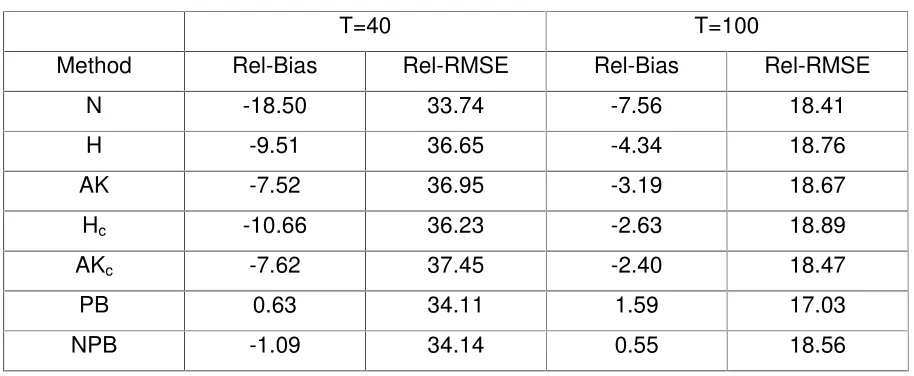
2- All the methods approximate the posterior S[O|y_(n)] of the hyper-parameters by the normal distribution, which is not always justified. This approximation stems from the asymptotic normality property of the MLE, but the distribution of the MLE can be skewed, particularly for short series, or when some of the hyper-parameters are close to their boundary values. Transformation of the hyper-parameters often improves the approximation, but only to a certain extent. Figure 1 shows the empirical distribution of the MLE of the logs of the state variance estimator,

x=0.5log q

ˆ

( )

ˆ

, for series of length 40 generated from the simple Gaussian ‘random walk plus noise model’. (See Section 4.1 for more details. The use of this transformation for model variances is very common, see e.g., Koopman et. al. 1995, Page 210). Testing the normality of this distribution yields p-values < 0.01 with all the common normality tests. The mean is -1.20, the median is -0.80 and the skewness is -5.04. The distribution of

x

ˆ

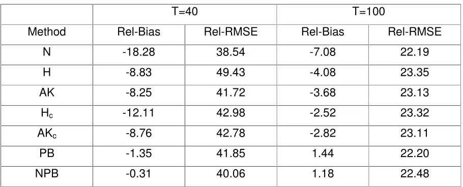
is much closer to normality when increasing the length of the series to 100, but even in this case the normality hypothesis is rejected by all the tests, with p-values < 0.01.

Figure 2 shows the empirical distribution of the logs of the MLE of the slope variance

2

R

V

under the BSM model defined by (4.4) for series of length 84, with true variance

2 _0.0024

R

V . As readily seen, the distribution is very skewed with mean, median and skewness equal to -9.68, -6.41 and -2.19 respectively, which in this case is explained by the proximity of the true variance to its boundary value. A similar picture is obtained even when increasing the length of the series to 240.

3- The computation of the Information matrix required for these methods may become unstable as the model becomes more complex and the number of unknown parameters increases. See Quenneville and Singh (200) for further discussion.

4- As already implied by the preceding discussion, all these methods basically assume that the model hyper-parameters are estimated by MLE or REML. This is not necessarily the case in practice and at least some of the parameters could be estimated by different methods, possibly using different data sources.

The use of the bootstrap methods overcomes the four disadvantages mentioned above. In particular, it produces estimators with bias of order O(1/n2), it does not rely on normality of the hyper-parameter estimators and is not restricted to MLE or REML estimators of the hyper-parameters (see Section 4.2). The empirical results in Section 4.1 further support the use of these methods.

3.4The Full Bayesian Approach

In the (empirical) Bayesian method mentioned in Section 3.3 the unknown hyper-parameters are first estimated by MLE or REML and then the PMSE is evaluated by computing the expectation of

{ ( )

P

_t

_O

_{[ ( )] }}ˆ2

t t

D D O over the posterior distribution

] | [_O y_(n)

S , see Equation (3.5). An alternative method of predicting the state vector and evaluating the PMSE is the use of the full Bayesian paradigm. The Bayesian solution consists of specifying a prior distribution S(O) for O and integrating the PMSE in (2.1) with respect to the posterior distribution _S[_O|y_(n)] yielding,

D

t

*

E

S[O|y(n)]

{

E

(

D

t

|

y

(n)

,

O

)}

E

[

D

t

|

y

(n)

]

(3.7) * { [( *) | , ]} [( *) | ( )]

2 )

( 2 ]

|

[ y_{( )} t t n t t n

t E E y E y

MSE _{S O n D D O D D}

for example, the article by Datta et al. (1999) for a recent implementation of the Markov Chain Monte Carlo (MCMC) approach with a model fitted to unemployment rates in the 50 States of the U.S.A.

4. EMPIRICAL RESULTS

4.1 Comparison of methods

This section compares the bootstrap methods with the methods discussed in Section 3 by repeating the simulation study performed by Quenneville and Singh (2000). The experiment consists of generating S=1000 series from the ‘random walk plus noise’ (RWN) model and estimating the PMSE of the empirical predictor

_D

ˆ

_t for every time point t by each of the methods. The RWN model is defined as,

2 2 1

,

;

~ (0,

) ,

~ (0,

)

t t t t t t t t

y

u

_H

u

u

_K

_H

N

_V

_K

N

_V

q

(4.1)

where

H

_t and

K

_t are mutually and serially independent. For the present experiment,

2 _{1,q 0.25}

V . The state value of interest is

D

_t

u

_t. Notice that the optimal predictor of

D

_t under the model with known variances does not depend in this case on

_V

2_{. The}

empirical predictor

_D

ˆ

_t is obtained by replacing q by its REML estimator

q

ˆ

in the expression of the optimal predictor, where

q

ˆ

is calculated by first calculating the REML

of

x=0.5log q

( )

and then defining

q = exp 2x

ˆ

( )

ˆ

. The restricted log likelihood equations

for state space models are developed in Tsimikas and Ledolter (1994, Equation 2.13). The REML

_V

_ˆ

2 _{required for the computation of the MSE estimators is available}

analytically as a function of

q

ˆ

, (the variance

_V

2 _{is concentrated out of the likelihood).}

We considered series of length 40 and 100 and computed the true PMSE of

_D

ˆ

_t for given t by simulating 50,000 series for each length;

MSE

_t

¦

50,000_i1

(

_D

ˆ

_{t i,}

_D

_{t i,}

) / 50,000

2 ,

1...

t

T

(

T

40,100

). For other computational details underlying this experiment see

Table 1 shows the mean percent relative bias (Rel-Bias) and mean percent relative root mean square error (Rel-RMSE) of the following MSE estimators: Na?ve (N), obtained by substituting

_{( , )}

_{ˆ ˆ}

2

u

q

V

for

_{( , )}

2

u

q

V

in the expression for the PMSE of the optimal predictor

( )

t

q

D

that employs the true variance; Ansley and Kohn (AK), defined by (3.4); Hamilton (H), defined by (3.6); The corrected estimators of Ansley and Kohn (AKc), and Hamilton

(Hc) developed by Quenneville and Singh (2000); parametric bootstrap (PB) developed

in Section 3.1 (Equation 3.1) and nonparametric bootstrap (NPB) described in Section 3.2. The results for the na?ve estimator, AK and AKc are based on 5000 simulated

series. The results for H, Hc and the bootstrap methods are based on 1000 simulated

series, drawing 2000 values

q

_i for H and Hc and generating 2000 bootstrap series for

each simulated series for the bootstrap methods.

Denote by

d

_{s t,}

[

MSE

ˆ

_{s t,}

MSE

_t

]

the error in estimating the true MSE at time t with series s by an estimator

MSE

ˆ

_{s t,} and let

d

_t

¦

1000_{s 1}

d

_{s t,}

/1000

,

1000

(2) 2

,

1

/1000

t _s s t

d

¦

d

. The

mean Rel-Bias and Rel-RMSE are defined as,

Rel-Bias

100

T_{t 1}

[ /

d MSE

_{t t}

]

T

¦

,

(2) 1/ 2 1

100

Rel-RMSE

T_t

[(

d

_t

) /

MSE

_t

]

[image:16.612.78.535.501.689.2]

T

¦

(4.2)

Table 1. Percent Mean Relative Bias and Relative Root MSE of PMSE Estimators for the RWN Model with Normal Errors

T=40 T=100

Method Rel-Bias Rel-RMSE Rel-Bias Rel-RMSE N -18.50 33.74 -7.56 18.41 H -9.51 36.65 -4.34 18.76 AK -7.52 36.95 -3.19 18.67 Hc -10.66 36.23 -2.63 18.89

AKc -7.62 37.45 -2.40 18.47

The first 6 estimators in Table 1 have been considered by Quenneville and Singh (2000) and even though we attempted to emulate their experiment exactly, the biases obtained in our study are always substantially lower than the biases reported in their article, including for the new methods AKc and Hc developed by them. However, the ordering of

the methods with respect to the magnitude of the bias is the same in both studies. (Quenneville and Singh do not report the MSE of the PMSE estimators).

The results in Table 1 show that the bootstrap methods are much superior to the other methods in terms of the bias, notably with the shorter series. The two bootstrap estimators also have lower RMSEs than the other methods proposed for reducing the bias of the na?ve estimator by about 6-8%, except for the long series where the use of NPB yields a similar RMSE to that of the other methods. Notice that the enhanced methods Hc and AKc proposed by Quenneville and Singh (2000) indeed reduce the bias

for the case T 100 (but not for T 40), but the Rel-RMSE are similar to the values obtained without the correction terms. An interesting outcome revealed from the table is that the na?ve estimator, although being extremely biased, has similar RMSE to those of the bootstrap estimators for T 40, and similar RMSE to NPB (and the other methods except PB) for T 100. This result is not surprising since the addition of correction terms to control the bias increases the variance. See also Section 4.2, and Singh et al.

(1998)for similar findings in a small area estimation study.

In order to study the sensitivity of the various methods to the normality assumptions underlying the Gaussian model, we repeated the same simulation study but this time by generating the random errors

H

_t and

K

_t in (4.1) from Gamma distributions. Specifically,

4

,

~

( , ) ;

16 3

5

,

~

(

25 2

, )

3

9 4

8

16 5

t

v

t

v

t

Gamma

t

w

t

w

t

Gamma

H

K

(4.3)

[image:18.612.79.534.133.317.2]

Table 2. Percent Mean Relative Bias and Relative Root MSE of PMSE Estimators for the RWN Model with Gamma Errors

T=40 T=100

Method Rel-Bias Rel-RMSE Rel-Bias Rel-RMSE N -18.28 38.54 -7.08 22.19 H -8.83 49.43 -4.08 23.35 AK -8.25 41.72 -3.68 23.13 Hc -12.11 42.98 -2.52 23.32

AKc -8.76 42.78 -2.82 23.11

PB -1.35 41.85 1.44 22.20 NPB -0.31 40.06 1.18 22.48

The biases displayed in Table 2 are quite similar to the biases in Table 1, indicating that the performance of the various methods is not sensitive to the normality assumptions. The Rel-RMSE, however, are higher in this case by about 17.5% for T 40 and 25% for

100

T . (The increase in Rel-RMSE for Hamilton’s method with T 40 is 35%.) The bootstrap methods again perform better than the other methods, particularly in terms of bias reduction. Notice that like in the Gaussian case, the na?ve PMSE estimator has the lowest Rel-RMSE despite being highly biased.

4.2 Application of the parametric bootstrap method with a model fitted to employment rates in the U.S.A.

In this section we apply the parametric bootstrap (PB) method to the model fitted by the Bureau of Labour Statistics (BLS) in the U.S.A. to the series Employment to Population

Ratio in the District of Columbia, abbreviated hereafter by EP-DC. The EP series consist

generating another set of bootstrap series). The unique feature of this experiment is that the model contains 18 unknown hyper-parameters estimated in 3 stages, with only 3 of the parameters being estimated by maximization of the likelihood.

4.2.1 Model and Parameter estimation

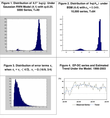
The EP-DC series is plotted in Figure 4 along with the estimated trend under the model defined below. This is a very erratic series: the irregular component (calculated by X12 ARIMA) explains 55% of the month to month changes and 32% of the yearly changes. A large portion of the irregular component is explained by the sampling errors. Let

y

t

define the direct sample estimate at time t and Y_t the corresponding true population ratio such that

e

t

y

t

Y

t is the sampling error. A state-space model is fitted to the series

y

_t that combines a model for Y_t with a model for

e

_t. The model postulated for Y_t

is the Basic Structural Model (BSM, Harvey, 1989),

Y_t L_t S_t I_t, I_t ~N(0,_VI2)

2

1 ; 1 , ~ (0, )

t t t t t Rt Rt R

L L R R R K K N V ¦

6 1 , ;

j jt

t S

S (4.4)

cos

sin

,

~

(

0

,

2

)

, , *

1 , 1

,

,t j jt j jt jt jt S

j

S

S

N

S

_Z

_Z

_K

_K

_V

S*_j,t sinZ_jS_{j,t 1} cosZ_jS*_{j,t 1}K*_j,t , K*_j,t ~N(0,V_S2)

Z_j 2S _j/12, j 1...6

The error terms I_t,K_Rt,K_j,tK*_j,t are mutually independent normal disturbances. In (4.1)

t

L

is the trend level,

R

_t is the slope and

S

_t is the seasonal effect. The model for the trend approximates a local linear trend, whereas the model for the seasonal effects uses the traditional decomposition of the seasonal component into 11 cyclical components corresponding to the 6 seasonal frequencies. The added noise enables the seasonal effects to evolve stochastically over time.

The model fitted to the sampling error is AR(15), which approximates the sum of an

design. By this design, households in the sample are surveyed for 4 successive months, they are left out of the sample for the next 8 months and then they are surveyed again for 4 more months. The AR(2) process accounts for the autocorrelations arising from the fact that households dropped from the survey are replaced by households from the same ‘census tract’. These autocorrelations exist irrespective of the sample overlap. The reduced ARMA representation of the sum of the two models is ARMA(2,17), which is approximated by an AR(15) model.

The separate models holding for the population ratios and the sampling errors are cast into a single state-space model as defined by (1.1) and (1.2). Note that the state vector consists of the trend, the slope, seasonal effects and sampling errors. The monthly variances of the sampling errors are estimated externally based on a large number of replications and considered as known, implying that the combined model depends on 18 unknown hyper-parameters. In order to simplify and stabilize the maximization of the likelihood, the AR(15) model coefficients are estimated externally by first estimating the autocorrelations of the sampling errors and then solving the corresponding Yule Walker equations (Box and Jenkins, 1976). The autocorrelations are estimated from the distinct monthly panel estimates as described in Pfeffermann et al. (1998). (A panel is defined by the group of people joining and leaving the sample in the same months. There are 8 panels in every month. The actual series is the arithmetic mean of the 8 panel series.)

Having estimated theAR(15) model coefficients, the three variances of the population model (4.4) are estimated by maximization of the likelihood, with the AR coefficients held fixed at their estimated values. The PB method for PMSE estimation accounts for the estimation of all the 18 unknown hyper-parameters, even though only 3 of them are estimated by maximization of the likelihood (see below).

4.2.2 Simulation Study

the series based on newly estimated hyper-parameters, and computed the empirical PMSE of these predictors. In the third phase we applied the PB method by generating 500 bootstrap series for each of 500 series selected at random from the 10,000 primary series. All the series are of length n=84, same as the length of the original series.

Phase A- Generation of primary series

As mentioned in Section 4.2.1, the actual series is the mean of 8 separate panel series. Hence, the first step of the simulation study was to generate 10,000 primary sets of 8 streams of sampling errors from the AR(15) model fitted to the original EP-DC series (see Table 3). Let ( )j

₍

_1...8,

_1...84)

tr

e

j

t

define the r-th set of stream sampling errors (r=1…10,000). Next we generated primary series of population values from the model (4.4), using again as hyper-parameters the variances estimated for the original EP-DC series, except for the irregular variance _Vˆ_I2, that was increased by a factor of 20 to make it similar to the sampling error variance. This was done in order to increase the differences between the trend and the seasonally adjusted estimators, and to test the performance of the PB method when applied to an even more variable series. The variances of the primary population model are, 2

_2.01,

2

_0.0024,

2

_0.0016

I R S

V

V

V

.

Denote by

Y

tr

(

r

1...10,000,

t

1...84)

the primary population series. Summing,

( )j ( )j

tr tr tr

y

Y

e

, j=1…8 yields 10,000 sets of 8 panel estimates.

Phase B- Computations for Primary Series

[image:22.612.80.544.133.298.2]

Table 3. AR(15) Model Coefficients of EP-DC Sampling Errors and Mean Estimates and Standard Deviations (SD) over 10,000 Simulated Series.

Lag 1 2 3 4 5 6 7 8

True Coefficients -0.588 -0.086 0.012 0.165 -0.127 -0.005 -0.025 0.048 Mean Estimates -0.587 -0.082 0.010 0.152 -0.118 -0.004 -0.022 0.042 SD of Estimates 0.042 0.047 0.047 0.047 0.047 0.046 0.046 0.046 Lag 9 10 11 12 13 14 15

True Coefficients -0.086 0.022 -0.089 -0.072 0.022 0.029 -0.026 Mean Estimates -0.076 0.019 -0.075 -0.057 0.019 0.024 -0.019 SD of Estimates 0.045 0.045 0.044 0.044 0.043 0.043 0.037

Next we computed for each month t the mean of the panel series ( )j tr

y

, yielding primary ‘observed series’

y

_tr

Y

_tr

e

_tr

(

t

1...84,

r

1...10,000)

. The three variances underlying the population model (4.4) have been estimated for each series by fitting the model to the series

y

_tr

(

t

1...84)

, fixing the AR(15) model coefficients at their estimated values. The variances were estimated by MLE, using the ‘prediction error decomposition’ for forming the likelihood (Harvey, 1989) and a quasi-Newton algorithm for the maximization process (same procedure as used by the BLS for the real series).

The computations in this study focus on the last time point, n=84. Let

D

84r define the

true component value of interest {L_84r or (

L

84r

,

84r)} for time n=84, as generated for primary series r (with hyper-parametersO Oˆ_{). Denote by D84r(O}ˆ_{r) the corresponding}

empirical predictor obtained by application of the Kalman filter with hyper-parameter estimatesOˆ_{r. The true PMSE is approximated as,}

¦ ! 000

, 10

1 84 84 2

84 r [ r(ˆr) r] /10,000

MSE D O D (4.5)

Phase C- Generation of Bootstrap Series and Computations

1- Generate 500 bootstrap series of stream sampling errors and population values using the hyper-parameters estimated in Phase B,

2- Estimate the AR(15) sampling error model coefficients and the population model variances for each of the bootstrap series,

3- Estimate the PMSE using the equations (3.1)-(3.2).

The procedures used for generating the bootstrap series in Step 1 and for estimating the hyper-parameters in Step 2 are the same as used for the primary series as described under Phase B. This process was repeated for each of the selected series, yielding 500 estimates of the true PMSE (4.5) computed in Phase B.

4.2.3 Results of Simulation Study

Table 4 shows the true root PMSE (R-PMSE) of the trend and seasonally adjusted predictors for time t=84 (Equation 4.5), and the bias and root mean square error (RMSE) of the PB PMSE estimators

MSE

ˆ

₈₄ (Equation 3.1). Also shown are the bias and

RMSE of the naive estimatorP₈₄( )_Oˆ, the estimator [2 ( )_{P84 O}ˆ_P84bs_{] of the contribution to} the PMSE resulting from ‘filter uncertainty’ (first component of 2.3, Equation C6 in Appendix C) and the estimator MSEˆ84,bsp of the contribution to the PMSE resulting from ‘parameter uncertainty’ (second component of 2.3, Equation C4 in Appendix C).

Table 4. Bias and Root MSE (

u

1000) of Estimators of PMSE of Trend and Seasonally Adjusted Predictors for time t=84. 500

u

500 replications

Trend Seasonally Adjusted

R-PMSE 1.481 1.581

Estimate

84

( )

ˆ

P

_O

MSEˆ84,bsp 2 ( )P84 OˆP84bs

MSE

ˆ

84

P

84

( )

O

ˆ

MSEˆ84,bsp 2 ( )P84 OˆP84bs

MSE

ˆ

84

The results displayed in Table 4 illustrate again the very good performance of the PB method in eliminating the large negative bias of the naive PMSE estimator. This result is particularly encouraging considering that we used for this study a complex model with 18 unknown hyper-parameters estimated by a three-step procedure. The estimators

84 ˆ 84

2 ( )_{P O P}bs _and

84,

ˆbs p

MSE also reduce the bias but each of these estimators only accounts for one component of the PMSE. Notice again that correcting the bias of the na?ve estimator does not necessarily imply a similar relative reduction in the RMSE. Thus, while the naive estimator has the largest RMSE in both parts of the table, the RMSE of the other three estimators are quite similar. As mentioned before, the addition of bias correction terms often increases the variance.

5. CONCLUDING REMARKS

The bootstrap method proposed in this paper for estimating the PMSE has four important advantages. First and foremost, it yields estimators with bias of correct order. Second, it does not require extra assumptions regarding the distribution of the hyper-parameters or their estimators, beyond the mild assumptions on the moments of the estimators. Third, it is not restricted to MLE or REML hyper-parameter estimators. Fourth, it is very general and can be used for a variety of models and prediction problems. We mention again that the other methods proposed in the literature for estimating the PMSE are restricted to MLE or REML hyper-parameter estimators and they either require the specification of prior distributions for the hyper-parameters, or that they assume that the hyper-parameters estimators have approximately a normal distribution. As illustrated by Figure 1 and 2, this assumption may not hold in practice.

estimates of variance of estimation errors in estimating the hyper-parameters”. In the discussion of this paper, A. Harvey makes a similar comment. Incorporating the proposed method for PMSE estimation into the simulation method underlying this approach seems natural but it requires further theoretical and empirical investigation.

APPENDIX A: TheKalman Filter andthe Innovation Form Representation

The Kalman filter consists of a set of recursive equations that are used for updating the predictors of current and future state vectors and the corresponding prediction error variance-covariance (PE-VC) matrices, every time that new data become available. The filter assumes known hyper-parameters. Below we consider the model defined by (1.1) and (1.2) with known hyper-parametersO.

Let

u

t"1

(

O

)

define the best linear unbiased predictor (BLUP) of

u

t#1 based on observations ($1) 1

...

$1

t

t

y

y

y

and denote by Pt%1 E u{[ t%1( )O ut%1][ut%1( )O ut%1] }c

_the

corresponding PE-VC matrix. The BLUP of

u

_t at time (t1) is ut_|t& ₁(O) Gtut& ₁(O), with

PE-VC Pt t| 1' G P Gt t'1 tcQt. When a new observation

y

t becomes available, the state predictor and the PE-VC are updated as,

1

| 1 | 1 | 1

( )

(

)

( ) ;

(

’

)

t t t t t t t t t t t t t t t

u

O

K y

I K Z u

O

P P

I Z F Z P

(

(

(

( (A1) where 1

| 1 t t t t t

K P Z F) ) c

_{, and} F_t Z P Z_{t t t| 1}* _tc 6_t is the PE-VC of the innovations

| 1 | 1

ˆ ( )

t t t t t t t t

v y y + y Z u + _O . By (A1) and the relationship

u

t t1|

( )

O

G u

t 1 t

( )

O

, , ,

y

_t

Z u

_{t t t| 1}-

( )

O

v

_t ;

u

t t1|

( )

O

G u

t 1 | 1t t

( )

O

G K v

t 1 t t

. . /

. (A2) The two equations in (A2) define the innovation form representation of the state-space model (1.1)-(1.2). The standardized innovations used for the NPB method are,

1/ 2

t t t

v

F

0

v

APPENDIX B: Rate of Convergence of

_{[ ( )}

ˆ

_{( )]}

2

t t

E

D O D O

Below we define conditions under which E[Dt(Oˆ)Dt(O)]2 (the second component of

the PMSE in 2.3) is of orderO(1/n), assuming for convenience that the matrices

Z

_t and

t

G

are known for all t. We first consider the case where the state vector of interest corresponds to the last time point with observations (

t

n

). Suppose that,

1- _{D O D On}( )ˆ _n( ) [ _{wD On}( ) /_{wO O O}] (c ˆ ) O_p(1/ )n and that the O_p(1/ )n term is negligible compared to the first term.

2-

E

[(

O O O O

ˆ

)(

ˆ

)’|

w

D O

_n

( ) /

w

O

]

V

( ) /

O

n o

_p

(1/ )

n

, where V( ) /_O n E[(_{O O O O}ˆ )(ˆ ) ]c

3- lim 1₁ , , n

n j n j j

n M M

1

2

354

¦

c < f, whereMn j, Rn Rn1 ... Rn j 1 (j 1... )n 6 687

u u u ; Rt (I K Z Gt t) t 4- The matrices [_wK_t/_wO] [F K_{t w t}/_wO]c are bounded for all

t

.

Conditions 1 and 2 are the same as in Ansley and Kohn (1986). Condition 1 is mild while Condition 2 will be true if (_Oˆ_O) is approximately independent ofD_n(O). Ansley and Kohn establish asymptotic independence between the two terms for ARMA models by showing that _Oˆ depends approximately equally on all the observations whereas

) (_O

Dn depends mostly on the observations around n, with the weights assigned to the

other observations decreasing exponentially as the distance from n increases. As shown next, this argument applies to more general state-space models satisfying Condition 3, which itself is not binding (see below).

To see this, rewrite the left-hand side equation in (A1) as ut(_O) Ktyt Rtut9₁(_O).

Repeated substitutions of this equation yields the relationship,

u_n(O) K_ny_n M_n,1K_n: ₁y_n: ₁M_n,2K_n: ₂y_n: ₂ ...M_n,n: ₁K₁y₁ M_n,nuˆ₀ (B1)

where uˆ₀ defines the initial state predictor. By Condition 3, 0 , ,

n j n j n

M ;

<

time series model. Note that if the model is time invariant in the sense that the matrices

t t t

t G Q

Z , ,₆ , are fixed over time, the Kalman filter converges to a steady state with V-C matrices P_tt= P, F_t F

~ ~

1

| (Harvey, 1989). In the steady state,Kt K, Rt R, illustrating

that in this case the weights in (B1) decay exponentially.

Comment: We computed the empirical correlations between the MLE of the three variances of the population model (4.4) and the trend and the seasonally adjusted estimators for time

n

84

, using the 10,000 primary series generated for the simulation

study. The largest correlation found was Corr(L₈₄,Vˆ_s2) 0.018, illustrating the approximate independence between the state vector and the MLE of the hyper-parameters under this model.

Proposition 1: Under the conditions 1-4, E[_Dn(_Oˆ)_Dn(_O)]2 O(1/n).

Proof: By Conditions 1 and 2 it is sufficient to show that E{[wD O_n( ) /w wO D O][ _n( ) /wO] }c is bounded, and since _{D On}( ) l u_{n n}c ( )_O , the problem reduces to showing that

{[ _n( ) / _i][ _n( ) / _j] }

E _wu _{O wO w}u _{O wO} c is bounded for all

1

d

i

,

j

d

m

where

m

dim( ).

O

Write the left hand side equation of (A1) for t=n as, un( )O G un n>1( )O K vn n where

v

n is defined below (A1). Differentiating both sides with respect to O_i yields,

wu_n( ) /_O w w_Oi R u_{n n}?₁( ) /_O w w_Oi [ K_n/w_Oi]v_n (B2)

The two terms in the right-hand side of (B2) are uncorrelated. To see this, write

1( ) [ 1 1( )]

n n n n n n n n n n n n

v y Z G u @ _O Z_{K H} Z G u@ u @ _O and note that unA1( )O E u( nA1|y( 1)nA ), implying that E v y( |n ( 1)nB ) 0 and

1 ( 1)

{[ _n ( ) / _i] |_{n n} } 0

E wu B _O w_{O Q} y B . It follows therefore that,

{[ ( ) / ][ ( ) / ] } {[ 1( ) / ][ 1( ) / ] }

( / ) ( / )

n i n j n n i n j n

n i n n j

E u u R E u u R

K F K

O O O O O O O O

O O

C C c

c c

w w w w w w w w

c

w w w w (B3)

1

, ,

1

{[ ( ) / ][ ( ) / ] } ( / ) ( / )

( / ) ( / )

n i n j n i n n j

n

n j n j i n j n j j n j j

E u u K F K

M K F K M

O O O O O O

O O

D

D D D

E

c c

w w w w w w w w

c c

¦

w w w w (B4)

The matrices (_wK_t/_wO) (F K_{t w t}/_wO)c are symmetric and positive semi-definite and by Condition 4 they are bounded, so that the proof is completed by means of Condition 3.

Comment: By assuming time invariant matrices Z_t Z G, _t G, ‘strong consistency’ of

ˆ

O (OˆoO a.s. as no f) and some other regularity conditions, Watanabe(1985) shows that

lim[ ( )

_n

ˆ

_n

( )] 0

n

p

_{D O D O}

FG

, employing a similar representation to (B1).

The analysis so far is restricted to the case where the state vector of interest corresponds to the last time point with observations,

t

n

. When

t

n

, the optimal state predictor and the corresponding PE-VC are obtained by application of an appropriate smoothing algorithm, and it is easy to verify that Proposition 1 holds in this case as well. One way to see this is by noticing that the smoothed state predictor for time t can be computed by augmenting the state vectors at times

(

t

1

)...

n

by the vector u_t and applying the Kalman filter to the augmented model. The smoothed predictor of u_t is then the (Kalman filter) predictor obtained for

u

t at the last time point,

n

, for which the proposition was shown to hold.

Finally, consider the case

t n

_!

and let

t n r r

,

_!

0

. In this case,

)

(

)

(

...

)

(

_{1 1 ,}

|n

O

n r n r n n

O

nr n

O

t

G

G

G

u

B

u

u

H

I

H

H ,

|

( )

ˆ

,

( )

ˆ

t n n r n

u

_O

B u

_O

, such that _{D O D Ot n|} ( )ˆ _{t n|} ( )

, [ ( )ˆ ( )] t n r n n

l B uc _O u _O . For Proposition 1 to hold in this case it is sufficient that the matrix

r n

B

_, is bounded, which would be the case if

r

is fixed. If, however,

r

is allowed to increase with

n

, it is necessary to require that _f

J

K

J

K Bnr B r

APPENDIX C: Proof of Theorem

By (2.3) the true PMSE is,

2 2 2

2

ˆ ˆ

[ ( ) ] [ ( ) ] [ ( ) ( )] ˆ

( ) [ ( ) ( )]

t t t t t t t

t t t

MSE E E E

P E

D O D D O D D O D O O D O D O

(C1)

Denote by E_* the expectation with respect to the bootstrap distribution (the distribution

over all possible bootstrap series generated with hyper-parameterOˆ_{). Then, analogously}

to (C1),

2 2 2

* * *

2 *

ˆ ˆ ˆ ˆ

[ ( ) ] [ ( ) ] [ ( ) ( )]

ˆ ˆ ˆ

( ) [ ( ) ( )]

b b b b b b b b

t t t t t t

b b b

t t t

E E E

P E

D O D D O D D O D O

O D O D O

(C2)

where b b t l ut t D c _; b

t

u _{is the true state vector of bootstrap series} b at time t and Db(Oˆ)

t

and D_tb(Oˆb) are the predictors of b t

D

using the ‘true’ parameter Oˆ and the estimator Oˆb respectively.

Under Condition

,,

of the theorem, E[_Dt(_Oˆ)_Dt(_O)]2 O(1/n)(see also Appendix B). Hence, using results from Hall and Martin (1988),

E{[_Dt(_Oˆ)_Dt(_O)]2 E_*[_Dtb(_Oˆb)_Dtb(_Oˆ)]2} O(1/n2) (C3) so that we can estimate,

2 2

, 1

1

ˆ ˆ ˆ

ˆ[ ( ) ( )] ˆ B [ ( )b b b( )] bs

t t _b t t t p

E MSE

B

D O D O

¦

L D O D O (C4)

Similarly, by Condition ,, E[Pt(Oˆ)Pt(O)] O(1/n). Hence,

E{[P_t(Oˆ)P_t(O)]E_*[P_t(Oˆb)P_t(Oˆ)]} O(1/n2) (C5) implying,

ˆ( )ˆ ( )ˆ 1 B₁[ ( )ˆb ( )] 2 ( )ˆ ˆ bs

t t b t t t t

P P P P P P

B