The relative importance of rainfall, temperature and yield data for a reginal-scale crop model

promoting access to White Rose research papers

White Rose Research Online [email protected]

Universities of Leeds, Sheffield and York

http://eprints.whiterose.ac.uk/

This is an author produced version of a paper published in Agricultural and Forest Meteorology

White Rose Research Online URL for this paper:

http://eprints.whiterose.ac.uk/id/eprint/78445

Paper:

Watson, J and Challinor, AJ (2013)The relative importance of rainfall,

temperature and yield data for a reginal-scale crop model.Agricultural and Forest Meteorology, 170. 47 - 57. ISSN 0168-1923

The relative importance of rainfall,

temperature and yield data for a

regional-scale crop model

Authors

4

James Watson1 and Andrew Challinor 5

Affiliation and Postal Address

6

Institute for Climate and Atmospheric Science 7

School of Earth and Environment 8

University of Leeds, United Kingdom 9

LS2 9JT 10

Keywords

11

Crop models; Climate models; Climate variability; Uncertainty; Crop yield; Data quality. 12

Abbreviations

13

a. GLAM – General Large-Area Model for Annual Crops 14

b. RMSE – root mean square error 15

c. RMSD – root mean square difference 16

d. YGP – yield gap parameter 17

e. TE – transpiration efficiency 18

f. p – bias rate 19

g. r – correlation coefficient of projected yield and observed yield 20

1

Abstract

When projecting future crop production, the skill of regional scale (> 100km resolution) crop models 22

is limited by the spatial and temporal accuracy of the calibration and weather data used. The skill of 23

climate models in reproducing surface properties such as mean temperature and rainfall patterns is 24

of critical importance for the simulation of crop yield. However, the impact of input data errors on 25

the skill of regional scale crop models has not been systematically quantified. We evaluate the 26

impact of specific data error scenarios on the skill of regional-scale hindcasts of groundnut yield in 27

the Gujarat region of India, using observed input data with the GLAM crop model. Two methods 28

were employed to introduce error into rainfall, temperature and crop yield inputs at seasonal and 29

climatological timescales: (1) random temporal resequencing, and (2) biasing values. 30

31

We find that, because the study region is rainfall limited, errors in rainfall data have the most 32

significant impact on model skill overall. More generally, we find that errors in inter-annual 33

variability of seasonal temperature and precipitation cause the greatest crop model error. Errors in 34

the crop yield data used for calibration increased Root Mean Square Error by up to 143%. Given that 35

cropping systems are subject both to a changing climate and to ongoing efforts to reduce the yield 36

gap, both potential and actual crop productivity at the regional scale need to be measured. 37

38

We identify three key endeavours that can improve the ability to assess future crop productivity at 39

the regional-scale: (i) increasingly accurate representation of inter-annual climate variability in 40

climate models; (ii) similar studies with other crop models to identify their relative strengths in 41

dealing with different types of climate model error; (iii) the development of techniques to assess 42

potential and actual yields, with associated confidence ranges, at the regional scale. 43

1. Introduction

All projections of the impacts of climate change on crop yield rely on models. Since such models are 45

incomplete representations of complex biological processes, their accuracy is limited by their 46

structure. Model accuracy is also limited by error (i.e. inaccuracy) and uncertainty (known 47

imprecision) in model inputs. Projections of crop yield using crop and climate models have identified 48

uncertainty in climate as a significant, if not dominant, contribution to total projected uncertainty 49

(e.g. Baron et al. 2005; Challinor et al., 2010, 2009a, 2005a; Cruz et al. 2007; Mearns et al. 2003; 50

Trnka et al., 2004). Lobell [this issue] finds that ignoring measurement errors when using an 51

empirical crop model can underestimate sensitivity to rainfall by a factor of two or more. These 52

sensitivities have clear implications for assessments of the impact of climate change on food 53

production and food security, and for the way in which adaptation options are formulated (e.g. 54

Challinor, 2009). 55

Calibration and weather inputs can have random or systematic errors at a variety of spatial and 56

temporal scales. For example, climate models can overestimate the number of rainy days whilst 57

underestimating rainfall intensity (Randall et al., 2007) and may also fail to represent the sub-58

seasonal variation in rainfall. Observational data such as crop production or daily weather may 59

contain uncorrelated, random errors introduced in measurement or recording, and systematic bias 60

from aggregation to the regional scale. These biases each have different implications for crop 61

While current efforts are underway to both quantify and reduce uncertainty in climate models (e.g., 63

the Coupled Model Intercomparison Project Phase 5), the specific impact of such errors on crop 64

models at the regional scale are still unknown. Crop models are often calibrated using historical 65

crop yield data, which is made available at the regional scale by organizations such as the Food and 66

Agriculture Organization of the United Nations (FAO) and the International Crops Research Institute 67

for the Semi-Arid Tropics (ICRISAT). Unlike climate model output, the quality and availability of this 68

data varies region by region. 69

The sensitivity of field-scale crop models to weather inputs has been assessed in a number of studies 70

(e.g. van Bussel et al., 2011; Dubrovsky et al., 2000), and the importance of calibration data in field 71

scale models has previously been analyzed (Batchelor et al., 2002). Sensitivity studies with regional 72

scale crop models, such as those reviewed by Challinor et al. (2009b), are less common. These 73

models integrate inputs at different scales, and are effectively test beds of theory about what 74

processes dominate variability in crop yield at these scales. Regional-scale models tend to be less 75

complex than field-scale models, therefore the impact of errors in input data on these two types of 76

model can be expected to differ. Berg et al. (2010) investigated the sensitivity of a large-scale crop 77

model to errors in rainfall inputs, but to date errors in rainfall, temperature and yield observations 78

have not been systematically studied at this scale. 79

Our objective in this study is to quantify the contribution made by specific data error scenarios to 80

error in regional scale yield projections. We take a published set of crop yield simulations (Challinor 81

et al., 2004), and introduce error into the input data in order to assess its impact on model error. 82

We use a set of simulations where regional-scale yields were reproduced skillfully using observed 83

weather data. The errors introduced to that data can be understood to represent uncertainty in the 84

simulation of weather by a climate model, and errors in the collection and collation of crop yield 85

information. The errors are introduced (i.e. simulated) at a range of temporal scales and using two 86

methods. The first samples and resequences values from the baseline climate to break temporal 87

structure (described in Section 2.2.1). The second alters the observed values such that they include 88

and then exceed observed values from the baseline climate (Section 2.2.2). Results from applying 89

these methods to rainfall, temperature and yield inputs are presented in Section 3.1, and a 90

comparison of these two schemes is given in Section 3.2. Three model configurations are used in the 91

study. These are described in Section 2.1 and the difference in results between these model 92

configurations is described in Section 3.3. The implications of the results for regional scale crop 93

modelling are discussed in Section 4 and conclusions are drawn in Section 5. 94

2. Material and Methods

2.1 Crop model

96

Crop yields were simulated using the General Large Area Model for annual crops (GLAM). This 97

model, which is freely available for non-commercial use via a licence agreement, has been used to 98

simulate the mean and variability of yields in current and future climates across the tropics (see 99

GLAM uses soil properties, a planting window, rainfall, solar radiation and minimum and maximum 101

temperature to simulate crop growth and development on a daily time step. It is calibrated by 102

adjusting the Yield Gap Parameter (YGP) to minimise discrepancies (as measured by Root Mean 103

Square Error, RMSE) between simulated and observed yields. Altering YGP alters the rate of change 104

of leaf area index with respect to time. We replicated the simulations of Challinor et al. (2004), 105

hereafter referred to as C2004. C2004 simulated groundnut yield across India on a 2.5 by 2.5 degree 106

grid for the period 1966 to 1989, using observed annual yield data for calibration and gridded 107

weather data derived from observations. Rainfall data were daily; the monthly temperature data 108

were linearly interpolated to produce the daily values required by GLAM. Solar radiation data were 109

monthly climatological solar radiation, which were linearly interpolated to daily values. Using these 110

data, C2004 were able to demonstrate the importance of both inter-annual and intra-seasonal 111

variability in rainfall in determining crop yield. The parameter set of C2004 is based on literature 112

searches to identify plausible ranges of parameters and subsequent minimisation of RMSE. All model 113

parameters lie near the centre of the ranges, with the exception of transpiration efficiency (TE). The 114

parameter set has subsequently been used and tested extensively (Challinor et al., 2009a, 2007, 115

2005a,b,c; Challinor and Wheeler 2008a,b). 116

The analysis presented here focuses on a grid cell in Gujarat (GJ) in which both the observed inter-117

annual variability in yield and the skill of the crop model in reproducing that variability was high 118

(correlation coefficient, r=0.74). The RMSE of the GJ grid cell is higher than that of the other two grid 119

cells examined in detail by C2004 (281 kg ha-1 as compared to 105 and 176 kg ha-1). However, both of 120

these grid cells, and many of the others simulated in C2004 had lower inter-annual variability in yield 121

than GJ, and also a lower correlation coefficient between observed and simulated yield. Thus the 122

choice was made to focus on a grid cell where GLAM has demonstrable skill in reproducing inter-123

annual variability, despite the absolute RMSE not being the lowest. 124

The replicated C2004 simulations for GJ were used as a control experiment. In all cases, unless 125

otherwise reported, the model was calibrated by varying YGP in steps of 0.05, from a minimum of 126

0.05 to a maximum of 1. The calibrated value of YGP is that which produces the lowest RMSE over 127

the whole time period. Note that variation in model skill when calibration and evaluation time 128

periods were separated was assessed by C2004, and found to be small. Replication of the original 129

results was not perfect, due to minor modifications made to the model code since 2004. C2004 130

reported a model yield RMSE in GJ of 281 kg ha-1, while the control simulation in the current study 131

gave a yield RMSE of 274 kg ha-1. Model skill was measured by two metrics: RMSE, and the 132

correlation coefficient of projected yield and observed yield (r). 133

Three crop model configurations were used in the study. Configuration A is taken directly from 134

C2004 and reproduces the yields from that study (subject to the minor differences noted above). 135

Configuration B is identical to A, but with the GLAM high temperature stress parameterisation of 136

Challinor et al. (2005c) activated. This configuration was used because the temperatures resulting 137

from some of the biases described in Section 2.2.2 below fall outside the range observed in the 138

baseline climate. In particular, they exceed the critical value beyond which anthesis and pod set are 139

affected. Configuration C is identical to B, but with the transpiration efficiency (TE) set to 2.5 Pa. This 140

new value is at the centre of the range of values identified from the literature by C2004. Since TE is 141

the only model parameter not found by C2004 to be near the centre of the range suggested by the 142

model was carried out. In these simulations, the primary impact of the use of yield data is through 144

the calibration parameter, YGP. Therefore, through comparing configurations A and C, conclusions 145

may be drawn on the importance of historical crop yield data in the development of model 146

parameterisations. 147

2.2 Simulating model input errors

148

Rainfall, temperature and yield model inputs were each perturbed using two methods. Random 149

temporal resequencing (referred to concisely as shuffling) of the primary data (daily rainfall, monthly 150

temperature and annual crop yield) was used to simulate errors where certain temporal information 151

is destroyed, but values remain consistent with the current climate. The second method biased the 152

primary input data across a range that includes, and also exceeds, values found in the baseline 153

climate. These two methods are described in detail in Sections 2.2.1 and 2.2.2. Both of these 154

methods were used to assess the impact of data errors on GLAM at three timescales: subseasonal, 155

seasonal and climatological. Minimum and maximum temperature values were perturbed 156

simultaneously in order to maintain consistency in the diurnal temperature range. Since we are 157

interested in the effect of errors in the input data available to the model, only the relevant 158

observations were perturbed – not the interpolated values. 159

2.2.1 Random shuffling of input data

160

In order to assess the importance of temporal information in GLAM’s input given the current 161

climate, values from the full June to September, 1966 to 1989, dataset were randomly shuffled at 162

three timescales, according to the following three operations: 163

1. Shuffle-Subseason: daily rainfall and monthly temperature values shuffled within a season, 164

which preserves inter-annual variability and climatology. 165

2. Shuffle-Season: rainfall, temperature and yield seasons shuffled as individual units (i.e., 166

keeping within-season values intact), which retains subseasonal information. 167

3. Shuffle-All: subseasonal and inter-annual variability in rainfall and temperature are both 168

altered by shuffling values across the entire dataset. 169

Yield calibration data were only included in Shuffle-Season, as only seasonal values exist. Each 170

shuffling operation was repeated using 1000 unique random number seeds, so that their aggregate 171

behaviour could be determined. GLAM was then run on each shuffled dataset in turn, where all 172

inputs were the same as in C2004 except for a single shuffled input type (i.e., the effect of rainfall, 173

temperature and yield shuffling were each tested separately). This procedure was repeated for 174

parameter configurations A, B and C. 175

2.2.2 Biasing input data

176

Biasing temperature, rainfall and yield allows the simulated errors to go beyond the range of values 177

of these variables that are observed in the current climate. Two options were considered for 178

assessing the impact of input data biases: using known climate model error to alter observed 179

weather, and systematically perturbing weather by introducing standardised noise. The first option 180

has the advantage of clear links to the current skill of climate models and the second has the 181

permits qualitative comparison of simulated error with existing climate model error, this method 183

was chosen. As with the shuffling, each input data variable was perturbed in isolation, to assess its 184

individual impact on crop model skill. Since the variables perturbed are in different units, we chose 185

to base the bias rate p on standard deviation, to permit comparison across variables. Standard 186

deviation is a commonly used aggregate variable characteristic which is in the same units as the 187

variable being considered. Biased values were randomly chosen from the normal distribution 188

defined by a reference value v and a standard deviation equal to p% of the standard deviation of the 189

input values being perturbed. For example, when p = 0%, the perturbed value will equal v, and as p

190

is increased, the likelihood of perturbed values being chosen further from v increase. 191

Datasets were perturbed at three timescales, using the following operations: 192

i. Bias-Day. Each daily rainfall value was perturbed independently of all other values. That is, 193

each input value v was replaced with a perturbed value v’ chosen from the normal 194

distribution with a mean of v and a standard deviation p% of the climatic rainfall standard 195

deviation. Note that the use of the term ‘bias’ here has been chosen to simplify the naming 196

scheme – this operation does not uniformly alter multiple values simultaneously. 197

ii. Bias-Season: A single adjustment of value d was applied to all input values across the entire 198

growing season in any one year. For rainfall and temperature inputs, d was chosen by 199

subtracting the seasonal mean from the value v’ selected from a normal distribution with 200

mean equal to the seasonal mean, and standard deviation equal to p% of the seasonal 201

standard deviation. Since only single yield values were available per season, biased yield 202

values were calculated according to their climatological standard deviation. 203

iii. Bias-Climate: All input values were uniformly altered by the single value d, chosen by 204

subtracting the climatological mean from a value chosen from the normal distribution with 205

mean equal to the climatological mean, and standard deviation equal to p% of the 206

climatological standard deviation. For temperature and precipitation, this climatological bias 207

represents an error in the simulation of the mean climate, with no error in inter-annual 208

variability. For yield data, it represents a systematic bias in the measurement of regional-209

scale crop yield data. 210

Each of these operations were performed for values of p ranging from 0 to 299, so that the impact of 211

biases chosen from distributions with up to three times the input standard deviation were tested. 212

As in Section 2.2.1, each perturbed variable was tested in isolation, with all other inputs the same as 213

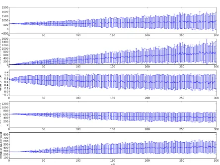
in C2004. GLAM was run on each biased dataset with 100 random number seeds. Figure 1 provides 214

an example illustration of the effect of climatological biases on these GLAM runs, while Table 1 215

summarizes the shuffling and bias experiments performed in this study. 216

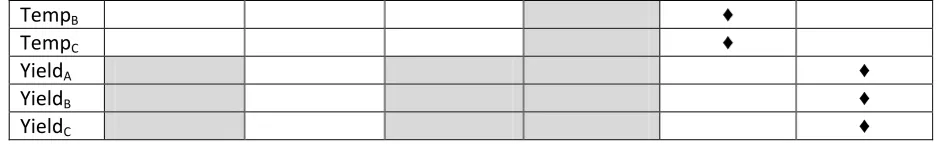
Table 1 Experiments performed for each input type and dataset operation. Shaded cells indicate studies that were not

217

performed. Operations that resulted in an average RMSE that differed from the result of the baseline simulation by

218

more than 50% are marked with a ♦.

219 Shuffle Subseason Shuffle Season Shuffle All Bias Day Bias Season Bias Climate

RainA ♦ ♦ ♦ ♦

RainB ♦ ♦ ♦ ♦

RainC

TempB ♦

TempC ♦

YieldA ♦

YieldB ♦

YieldC ♦

220

3.

Results

An overview of the input data operations that, on average, resulted in more than 50% difference in 222

RMSE is shown in Table 1. While this average effect on RMSE is a crude indicator of the impact of 223

each data operator on GLAM’s performance, characteristics such as GLAM’s resilience to varying 224

degrees of perturbation types, and the relative spread of behaviours across random seeds, are key 225

to understanding the true impact of these errors at the regional scale. This section describes these 226

results, and compares the relative impact of data operations across input variables. 227

3.1 Impact of temperature, rainfall and yield error on model skill

228

Figure 2 shows the results of shuffling, in turn, temperature, precipitation and yield in model 229

configuration A. In the vast majority of cases, introducing error into these variables increases the 230

RMSE of the simulated yield. The largest impact on RMSE comes from shuffling rainfall seasons. 231

Shuffling of temperature seasons also results in RMSE that, in the vast majority of cases, is greater 232

than that of the control simulation. Shuffling of temperature and rainfall on subseasonal timescales 233

both result in similar changes to RMSE. 234

The correlation between simulated and observed yield is also plotted in Figure 2. Altering seasonal 235

total rainfall has by far the greatest effect on r, with yield and temperature perturbations having the 236

smallest effect. For both rainfall and temperature, increases in RMSE are associated with decreases 237

in correlation. Thus the increase in RMSE is due primarily to increased error in simulating the inter-238

annual variability of yield, as opposed to being associated with increased error in the simulation of 239

mean yield. In the case of perturbed yield input, there is far less evidence of any inverse relationship 240

between RMSE and correlation coefficient. This is because the calibration parameter, YGP, affects 241

mean yield more than it affects inter-annual variability. 242

The box and whiskers diagrams in Figure 2 have a smaller number of component time series for yield 243

than for either temperature or precipitation: there are 17 unique time series of yield, compared to 244

1000 for Shuffle-Season of both temperature and precipitation. This is a direct result of the 245

calibration procedure, whereby YGP is incremented in steps of 0.05; a smaller increment would 246

result in more time series. The difference in sample size between yield and the other two variables 247

does not affect the character of the results (see Section 3.3). 248

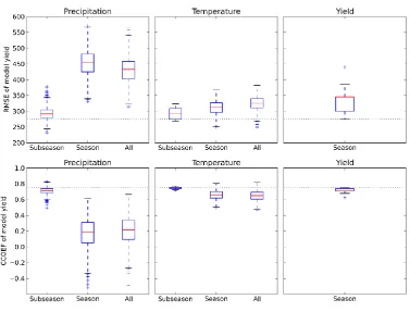
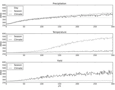
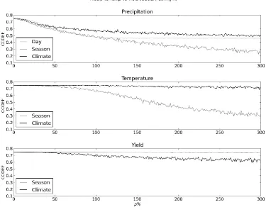
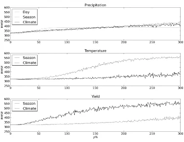
The impact of input data bias on model skill is presented in Figures 3 (RMSE) and 4 (correlation 249

coefficient). Each figure shows the impact averaged over all 100 random seeds. For p < 100, rainfall 250

biases had a greater effect on model skill, as measured by both of these metrics, than either 251

temperature or yield biases. At these low values of p, daily, seasonal and climatological rainfall 252

yield and temperature than it does for rainfall. For p < 50, this compensation is almost complete: 254

temperature and yield errors have no significant impact on model skill. 255

256

For p > 100, seasonal biases to temperature begin to significantly affect model skill, as measured by 257

both correlation coefficient and RMSE. This loss of skill is caused by greater inter-annual variability in 258

crop duration, which results in inter-annual variability in yield no longer being dominated by 259

precipitation. In contrast, climatological biases to temperature do not on average significantly affect 260

model skill, because the calibration procedure compensates for the mean bias in temperature. 261

Similar behaviour is seen for rainfall: climatological biases to rainfall are more easily compensated 262

for by calibration than seasonal biases. This is particularly evident in the correlation coefficient 263

(Figure 4); though it can also be seen in RMSE (Figure 3). The behaviour of yield biases for p > 100 264

contrasted with that of temperature: seasonal biases to yield do not affect model skill and 265

climatological biases do. This is a direct result of the calibration procedure, which is based on yields 266

averaged over the whole time period. 267

3.2 Comparison of bias and shuffle schemes

268

The two schemes used to introduce error in this study are not directly comparable. In order to 269

provide some indication of the relationship between the schemes, an analysis was conducted. 270

Climatological mean monthly temperature was computed for each perturbation scheme in turn, and 271

for the observed data. The percentage of random number seeds that produced at least one value 272

outside the observed range (OR) was calculated. This was repeated for cumulative monthly

273

precipitation. The results varied by month, variable and scheme. Shuffle-Season, by definition, 274

produced no values outside of current climatology. Shuffle-Subseason produced relatively high 275

values for temperature (52 to 75%, across the four months) and September rainfall (93%) and 276

relatively low values for June, July and August precipitation (24.2, 0 and 1.3%, respectively). A similar 277

pattern was seen for Shuffle-All. 278

The results for the bias scheme are too numerous to report. In general, OR increased with increasing

279

p. A comparison between the shuffle and bias schemes was made by incrementing p from zero 280

upwards and noting the first value at which OR (biased) > OR (shuffled). For precipitation, this

281

occurred mostly at low values of p: 0 or 1 for June to August; 35 for September Bias-Season; and the 282

condition was not met for September Bias-Climate. For temperature, p was higher: 9-19 for Bias-283

Season and 180 for Bias-Climate. Whilst in many cases OR (biased) becomes comparable to OR

284

(shuffled) at relatively low values of p, the variation in the values of OR across months and variables

285

suggests that it is impossible to determine even a guideline range of values of p which may be 286

equivalent to the shuffled data. 287

A clearer distinction between the shuffle and bias schemes can be found by assessing the results 288

qualitatively. For example, for p < 150, any type of rainfall bias has a greater impact on RMSE than 289

either temperature or yield. This is consistent with the shuffle simulations at all timescales except 290

one: Shuffle-Subseason produces a significantly lower reduction in model skill than Bias-Day. By 291

altering seasonal totals, Bias-Day degrades model performance in a manner not seen in the 292

equivalent shuffle simulations. The fact that shuffle simulations either maintain or destroy the 293

temporal structure of variables is perhaps the clearest difference between this scheme and the bias 294

3.3 Comparison of model configurations

296

Model configurations A and B, which differ only in the activation of the high temperature stress 297

module, produced equivalent model behaviours for both the shuffled and biased operations. The 298

temperature data used in this study are monthly, with no attempt to reproduce observed daily 299

extremes. Thus this equivalence is not surprising. Model configurations A and C produce different 300

results in both the shuffled and biased cases. With no biasing or shuffling of input data, the RMSE of 301

these two configurations is 274 and 322 kg ha-1, respectively. Thus RMSE increases by 17.5% when a 302

value of transpiration efficiency from the centre of the observed range is used instead of the 303

calibrated value. The increase in RMSE would be larger if the value of YGP were not calibrated using 304

yield data. At p=0 the yield gap parameter was 0.8 for the control simulation (i.e. configuration A 305

with no bias or shuffling), and 0.2 for the corresponding simulation of configuration C. This 306

difference is the result of calibration compensating for the higher value of TE. 307

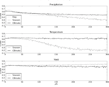
The performance of the shuffled configuration C simulations is shown in Figure 5. The broad 308

response of rainfall and temperature across the timescales is similar to that of configuration A. 309

However, unlike configuration A, RMSE was reduced and correlation coefficient increased by 310

subseasonal shuffling. Also, shuffling temperature both subseasonally and seasonally (i.e. Shuffle-All) 311

produces a lower RMSE than Shuffle-Season alone. Subseasonal shuffling, on average, makes the 312

seasonal distribution of values more uniform than observations, and therefore less realistic. These 313

results are therefore further manifestations of incorrect model calibration. 314

Since yield is a calibration input, the Shuffle-Season perturbation produced a limited number of 315

unique model results. Configuration A produced 17 unique yield projections, with RMSE of 317, 346 316

and 387 together accounting for 72% of the 1000 different seeds. Configuration C resulted in 2 317

unique yield projections – one with a RMSE of 370 (863 occurrences) and the other with RMSE of 318

323 (137 occurrences). This is a direct result of the calibration procedure, whereby the yield gap 319

calibration parameter is incremented in steps of 0.05. YGP decreases between configurations A and 320

C, in order to compensate for the higher value of transpiration efficiency. A step of 0.05 at lower 321

values of YGP will result in greater changes in simulated yield than the same step at higher values of 322

YGP, thus producing less unique yield time series with the higher transpiration efficiency of 323

configuration C. In order to test whether or not the difference between the baseline RMSE of 324

configurations A and C is an artefact of the chosen YGP increment of 0.05, these simulations were 325

repeated with a YGP increment of 0.01 (ie 99 simulations with YGP varied between 0.01 and 1). 326

Similar results were found: RMSE of 274 for configuration A and 318 for C, as compared to 274 and 327

322 respectively for a step of 0.05. 328

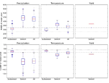
Figure 6 presents the results from the bias simulations for configuration C. As was the case for 329

shuffle operations, the character of the response of RMSE to rainfall, temperature and yield bias 330

errors was similar for configurations A and C. The seasonal and climatic yield biases resulted in 331

significantly higher RMSE in configuration C compared to A at all values of p. For temperature and 332

precipitation, this difference was less marked. For precipitation, the rate of increase in RMSE in 333

4. Discussion

4.1 The importance of calibration data

336

The interaction between model configuration and errors in rainfall, temperature and yield 337

calibration data (Section 3.3) demonstrates the importance of both crop yield data and observed 338

weather data. Without both of these data sources, it would have been impossible to determine 339

where the optimal value of transpiration efficiency lay. Errors resulting from this omission would 340

then be compounded by errors in observed yield, which is also used in the calibration procedure. 341

The yield calibration data in this study contributed to the skill of the model in two ways: (1) selection 342

of crop model parameters at a country scale (configuration A vs configuration C), and (2) as the basis 343

of regional calibration. Configuration C provides an estimate of the impact on RMSE of having 344

insufficient data to determine a value of transpiration efficiency that is appropriate for a regional-345

scale groundnut model in India. The increase in RMSE of 17.5% when switching to the non-calibrated 346

value of TE demonstrates the importance of regional-scale yield data in the development of 347

parameterisations within regional-scale crop models. This is in addition to the important role of yield 348

data in regional calibration and evaluation of models. In the current study, the largest increase to 349

RMSE that was induced by introducing errors to the crop yield calibration data was 143% (Bias-350

Climate, p=113). For comparison, the largest increase to RMSE induced by the shuffle scheme was 351

60%. The role of yield data for calibration is made more important by climate change, which will 352

affect both observed yields and transpiration efficiency, as well as other regional-scale crop 353

parameters that have not been assessed here. 354

If differences in RMSE across model configurations are comparable to the uncertainty in the 355

measurement of yield, then it is impossible to conclude which configuration is the most skilful. Since 356

the yield data do not have error bars, this comparison is difficult to make. Some indication of 357

uncertainty in yield measurement may come from comparing datasets. The Root Mean Square 358

Difference (RMSD) between the all-India groundnut yield data of the Food and Agriculture 359

Organization and that of the ICRISAT data (both used in C2004) is 33 kg ha-1, 4% of the mean yield of 360

either time series. The RMSD between configurations A and C is 96 kg ha-1, which is 15% of the mean 361

yield. Comparison of these two results suggests that the difference between configurations A and C 362

is significant. However, disagreement across datasets of observed yields is often greater than 4%. 363

Nicklin (in preparation) has shown that the RMSD between available groundnut yield datasets in 364

Mali vary by region and are between 83 kg ha-1 _{and 342 kg ha}-1_. 365

The importance of yield data for model calibration and evaluation will likely increase as climate 366

continues to change and as efforts to increase yields continue. These independent, but connected, 367

drivers of crop productivity continually alter the baseline situation that crop-climate models seek to 368

reproduce. The role of closing yield gaps in promoting food security has been noted by many authors 369

(e.g. Lobell et al., 2009). Bhatia et al. (2006) estimate that the yield gap for groundnut varies 370

significantly across Gujarat: 1180 to 2010 kg ha-1, which is 103-175% of the mean yield across the 371

region. Without monitoring of the yield gap, the contribution of climate variability and change to 372

crop productivity will be impossible to determine. Without assessments of the accuracy of yield 373

data, it is impossible to determine how much error is introduced to regional-scale crop models 374

4.2 Relative importance of rainfall, temperature and yield data

376

The importance of weather data to crop modelling is well established. Depending on the crop and 377

region under consideration, the relative impact of data quality of these input variables varies. Lobell 378

and Burke (2008) found that uncertainties in temperature generally had more of an effect than 379

uncertainties in precipitation across 94 crop-region combinations. Mearns et al. (1996) found that 380

simulated wheat yields were sensitive to changes in both temperature and precipitation, which 381

depended on soil characteristics. Nonhebel (1994a) found that temperature and solar radiation data 382

errors generated up to 35% overestimation of yield. In water-limited conditions, the model was 383

sensitive to inaccuracies in precipitation and solar radiation data, but when there was sufficient 384

water, it was sensitive to errors in temperature and solar radiation data (1994b). Heinemann et al. 385

(2002) found variations in simulated yield for soybean (up to 24%), groundnut (up to 13.5%), maize 386

(up to 7.6%) and wheat (up to 2.7%) resulting from errors in rainfall observations. Berg et al. (2010) 387

found that the frequency and intensity of rainfall, as well as cumulative annual rainfall variability, are 388

key data features for crop models to have skill in water-limited regions. In the current study rainfall 389

is found to be more important than temperature in simulating crop yield (Section 3.1). This is 390

consistent with the rainfed monsoon environment in Gujarat. 391

A more detailed analysis of the relative importance of rainfall, temperature and yield data in this 392

study requires some understanding of how the shuffle and bias schemes can be compared. Whilst 393

interpretation of the shuffle experiments in bias space is not trivial (Section 3.2), some comparisons 394

can be made. Figure 8 shows the performance of configuration A for both shuffle and bias 395

operations at the seasonal timescale. The bias results are those with the closest mean RMSE to the 396

corresponding shuffle simulation. Following Taylor (2001), Figure 8 illustrates the relationship 397

between the correlation coefficient, standard deviation and RMSE of observed and simulated yields. 398

Errors in precipitation, whether induced through random temporal resequencing (i.e. shuffling) or 399

through biasing, produced the largest systematic difference from observed yield. 400

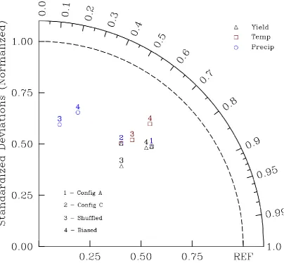
Two other differences are clear from Figure 8: for all variables (i.e. temperature, yield and rainfall) 401

shuffling results in a lower standard deviation in yield than biasing (points 3 vs points 4 in the figure); 402

and the use of non-calibrated TE (point 1 vs point 2 on the figure) significantly alters simulated 403

yields. The second of these results is discussed in Section 4.1. The first result indicates an important 404

difference between the two methods of error introduction. In all simulations, the standard deviation 405

in yield is lower than observations; but this is particularly true of the shuffled simulations. Associated 406

with this lower standard deviation is a lower correlation between observed and simulated yields. 407

Thus, by directly altering the temporal structure of the rainfall, temperature or yield data, the 408

seasonal shuffle operation has a greater impact on the skill of the model in simulating inter-annual 409

yield variability when compared to bias operations that result in a similar RMSE. 410

In order to assess the implications of the results presented above for operational crop forecasting, it 411

is necessary to compare the errors simulated here to those found in climate models. Section 4.1 412

briefly discusses such an analysis for yield data. In order to assess temperature and precipitation, the 413

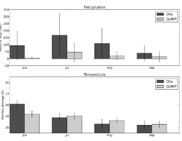
HadCM3 historical climate simulation of Collins et al. (2010) was analysed. Figure 9 compares the 414

observations used in this study to the HadCM3 simulation. The seasonal cycle of monthly 415

precipitation is captured by the climate model, but there is a significant dry bias. This is consistent 416

with the findings of Ines and Hansen (2006). The HadCM3 temperature data are closer to 417

It is not possible to associate a single value of p with the HadCM3 simulation. However, using 419

observations as a reference point, some values of p that are associated with the HadCM3 run can be 420

calculated. This was carried out as follows. Climatological mean monthly temperature was computed 421

for the observed data, for HadCM3, and the synthetic biased data. The RMSD of the observed 422

monthly values and those of each of the synthetic time series was calculated. The value of p that 423

produced the RMSD closest to the RMSD of HadCM3 and observations (p3) was recorded. The

424

procedure was repeated for monthly cumulative rainfall. For climatological means, the resulting 425

values of p3 for temperature were 271 for Bias-Season and 238 for Bias-Climate. For rainfall, p3 was

426

77 and 66, respectively. The low values of p3 for precipitation are the result of the high standard

427

deviation in the observed values (see Figure 9) that are used to scale p. When inter-annual variability 428

in rainfall was assessed in the error metric, by repeating the entire procedure using monthly 429

standard deviation in lieu of mean values, p3 values were 168 and 293 for Season and

Bias-430

Climate respectively. Taken together, these results suggest that the range of values of p used in this 431

study is consistent with the errors observed in climate models. 432

4.3 Generality of results

433

A number of factors that are specific to the current study affect the extent of applicability of the 434

results found. These fall into three categories: the crop model chosen, the location chosen, and the 435

perturbation operators used. GLAM does not account for non-climatic drivers of yield. Where biotic 436

stresses dominate, these results are likely not relevant. Also, since Gujarat is a water-limited 437

environment, the numerical analyses presented here are only relevant for rainfed environments, 438

where water availability is the main determinant of yield. Furthermore, the experiments of this 439

study were designed to allow comparison of the perturbations across different input variables, but in 440

some cases the perturbations differed across variables. For example, the distribution of values in the 441

rainfall dataset differ from the temperature values, so the equivalent Bias operations can have 442

differing effects. Ideally, we would have the same perturbation scheme applied to all variables 443

(comparable methods) which would have the same effect wherever applied (comparable effects). 444

With current methods, we can only choose one of these. For this study we have chosen comparable 445

methods, since if we had employed different methods, the differences resulting from perturbations 446

would have been due to methodological as well as numeric-specific issues like the example 447

described above. 448

Despite these limitations to the generality of results, some broader conclusions are possible. In 449

particular, the relationship between climate model bias and crop model calibration is worthy of 450

some discussion. 451

Yield data are required in order to calibrate any crop model. In the current study, YGP was used as a 452

process-based and time-independent calibration parameter to minimise RMSE between observed 453

and simulated yields. This process can correct a significant amount of climatological bias in 454

temperature, but is less effective for the systematic errors in yield or precipitation data in this study 455

(Figure 3). However, for precipitation, all three Bias perturbations in this study produce more wet 456

than dry biases; and the ability of YGP to compensate for systematic dry bias has been shown to be 457

greater than that for wet bias (Challinor et al., 2005d). Note also that the analysis presented in this 458

paper likely underestimates the importance of temperature, since the simulations are based on 459

of daily minimum and maximum temperature may have resulted in heat stress, which would have 461

had an influence on the RMSE of the configuration B and C simulations. 462

Whilst every crop model has its own equations, parameters and calibration procedure, common 463

characteristics may be expected across models. Any aspect of climate or weather that has been 464

proved to be an important determinant of crop yield will be an important quantity for a climate 465

model to simulate, regardless of the crop model used. Thus the importance of seasonal rainfall for 466

crop simulation is not specific to GLAM. Similarly, yield data are a crucial part of the calibration and 467

evaluation of any crop model. However, differences in model formulation mean that the relative 468

importance of temperature, precipitation and calibration data will vary between models. Many 469

models are more complex than GLAM and therefore have a higher number of crop-specific 470

parameters that can interact with each other. A complete treatment of these interactions is beyond 471

the scope of this study. Here, we investigated only two parameters (YGP and TE) at the regional 472

scale, and have therefore most likely produced a minimum estimate of the importance of 473

interactions between calibration parameters in other crop models. 474

5. Conclusions: improving the skill of crop-climate simulations

The results from this study suggest that errors in the inter-annual variability of seasonal temperature 476

and precipitation are likely to cause greater crop model error at the regional scale than systematic 477

bias in the simulation of climate. This study is based on one crop model alone. Similar studies with 478

other crop models would not only assess the robustness of the results, but may also identify the 479

relative strengths of crop models in dealing with different types of climate model error. 480

Regional-scale yield data for crop model calibration are central to the future of crop productivity 481

assessments. We found increases in crop model RMSE of up to 143% when the observed yield data 482

used for calibration were perturbed. Without assessments of the accuracy of yield data, it is 483

impossible to determine how much error is introduced to regional-scale crop models through the 484

calibration procedure. Where possible, confidence ranges should therefore be provided with 485

observed yield data. Ongoing efforts to close the yield gap, coupled with changes in climate and 486

other environmental drivers, mean that the monitoring of potential yields is also crucial. Without 487

estimates of the yield gap, the contribution of climate variability and change to crop productivity will 488

be impossible to determine. The spatial heterogeneity in the yields of many cropping systems is 489

significant. Thus improved measurement of actual and potential yields at the regional scale involves 490

not only improved monitoring, but also carefully developed geo-spatial techniques. 491

The results of this study suggest three key endeavours for improved assessment of future crop 492

productivity at the regional-scale: (i) increasingly accurate representation of inter-annual climate 493

variability in climate models; (ii) similar studies with other crop models to identify their relative 494

strengths in dealing with different types of climate model error; (iii) the development of techniques 495

Acknowledgments

Thanks to Ed Hawkins (University of Reading), Chris Ferro (University of Exeter), Tom Osborne 498

(University of Reading) and Kathryn Nicklin (University of Leeds) for insightful discussion. This work 499

was supported by the Natural Environment Research Council (NERC). 500

References

Baron, C., B. Sultan, M. Balme, B. Sarr, S. Teaore, T. Lebel, S. Janicot, and M. Dingkuh, 2005: From 502

GCM grid cell to agricultural plot: scale issues affecting modeling of climate impacts. Phil. Trans. Roy. 503

Soc. B, 1463 (360), 2095-2108. 504

Batchelor, W.D., Basso, B., and Paz, J.O. (2002). Examples of strategies to analyze spatial and 505

temporal yield variability using crop models. Eur. J. of Agron., Vol. 18, Issues 1-2, pp 141-158. 506

Berg, A., Sultan, B. and de Noblet-Ducoudré, N. (2010). What are the dominant features of rainfall 507

leading to realistic large-scale crop yield simulations in West Africa? Geophys. Res. Lett., 37, L05405. 508

Bhatia V.S., Singh Piara, Wani S.P., Kesava Rao A.V.R. and Srinivas K. (2006). Yield gap analysis of 509

soybean, groundnut, pigeonpea and chickpea in India using simulation modeling. Global Theme on 510

Agroecosystems Report No. 31. Patancheru 502 324, Andhra Pradesh, India: International Crops 511

Research Institute for the Semi-Arid Tropics (ICRISAT). 156 pp. 512

Challinor, A. J., T. R. Wheeler, J. M. Slingo, P. Q. Craufurd and D. I. F. Grimes (2004). Design and 513

optimisation of a large-area process-based model for annual crops. Agr. For. Met., 124, (1-2) 99-120. 514

Challinor, A. J., T. R. Wheeler, J. M. Slingo and D. Hemming (2005a). Quantification of physical and 515

biological uncertainty in the simulation of the yield of a tropical crop using present day and doubled 516

CO2 climates. Phil. Trans. Roy. Soc. B. 360 (1463) 1981-2194 517

Challinor, A. J., T. R. Wheeler, J. M. Slingo, P. Q. Craufurd and D. I. F. Grimes, (2005b). Simulation of 518

crop yields using the ERA40 re-analysis: limits to skill and non-stationarity in weather-yield 519

relationships. J. App. Met. 44 (4) 516-531. 520

Challinor, A. J., T. R. Wheeler, P. Q. Craufurd, and J. M. Slingo (2005c). Simulation of the impact of 521

high temperature stress on annual crop yields. Agr. For. Met, 135 (1-4) 180-189 522

Challinor, A.J., Slingo, J.M., Wheeler, T.R. and Doblas-Reyes, F.J. (2005d). Probabilistic simulations of 523

crop yield over western India using the DEMETER seasonal hindcast ensembles. TELLUS A, 57, 498-524

512. 525

Challinor, A. J., T. R. Wheeler, P. Q. Craufurd, C. A. T. Ferro and D. B. Stephenson (2007). Adaptation 526

of crops to climate change through genotypic responses to mean and extreme temperatures. Agr. 527

Eco. Env., 119 (1-2) 190-204 528

Challinor, A. J. and T. R. Wheeler (2008a). Use of a crop model ensemble to quantify CO2 stimulation 529

Challinor, A. J. and T. R. Wheeler (2008b). Crop yield reduction in the tropics under climate change: 531

processes and uncertainties. Agr. For. Met., 148 343-356 532

Challinor, A. J. (2009). Developing adaptation options using climate and crop yield forecasting at 533

seasonal to multi-decadal timescales. Env. Sci. Pol. 12 (4), 453-465 534

Challinor, A. J., T. R. Wheeler, D. Hemming and H. D. Upadhyaya (2009a). Ensemble yield simulations: 535

crop and climate uncertainties, sensitivity to temperature and genotypic adaptation to climate 536

change. Clim. Res., 38 117-127 537

Challinor, A. J., F. Ewert, S. Arnold, E. Simelton and E. Fraser (2009b). Crops and climate change: 538

progress, trends, and challenges in simulating impacts and informing adaptation. J. Exp. Bot. 60 (10), 539

2775-2789. doi: 10.1093/jxb/erp062 540

Challinor, A. J., E. S. Simelton, E. D. G. Fraser, D. Hemming and M. Collins (2010). Increased crop 541

failure due to climate change: assessing adaptation options using models and socio-economic data 542

for wheat in China. Env. Res. Lett. 5 (2010) 034012 543

Collins M, Booth B.B.B., Bhaskaran B., Harris G., Murphy J. M., Sexton D.M.H. and Webb M.J. (2010). 544

Climate model errors, feedbacks and forcings: a comparison of perturbed physics and multi-model 545

ensembles. Clim. Dyn. 546

Cruz, R.V., H. Harasawa, M. Lal, S. Wu, Y. Anokhin, B. Punsalmaa, Y. Honda, M. Jafari, C. Li and N. Huu 547

Ninh (2007): Asia. Climate Change 2007: Impacts, Adaptation and Vulnerability. Contribution of 548

Working Group II to the Fourth Assessment Report of the Intergovernmental Panel on Climate 549

Change, M.L. Parry, O.F. Canziani, J.P. Palutikof, P.J. van der Linden and C.E. Hanson, Eds., Cambridge 550

University Press, Cambridge, UK, 469-506. 551

Dubrovsky, M., Zalud, Z. and Stastna, M. (2000). Sensitivity of ceres-maize yields to statistical 552

structure of daily weather series. Clim. Chan., Vol. 46, Issue 4, 447-472. 553

Heinemann, A. B., Hoogenboom, G. and Chojnicki, B. (2002). The impact of potential errors in rainfall 554

observation on the simulation of crop growth, development and yield. Eco. Model., Vol. 157, No. 1, 555

1-21. 556

Ines, A.V.M. and Hansen, J.W. (2006). Bias correction of daily GCM rainfall for crop simulation 557

studies. Agr. For. Met., Vol. 138, No. 1-4, 44-53. 558

Lobell, D.B. and Burke, M.B. (2008). Why are agricultural impacts of climate change so uncertain? 559

The importance of temperature relative to precipitation. Env. Res. Lett., Vol. 3, No. 3. 560

Lobell, D.B., Cassman, K. G. and Field, C.B. (2009). Crop yield gaps: their importance, magnitudes, 561

and causes. Ann. Rev. Env. Res., Vol. 34, 179-204. 562

Mearns, L. O., Rosenzweig, C. and Goldberg, R. (1996). The effect of changes in daily and interannual 563

climatic variability on CERES-Wheat: A sensitivity study. Clim. Chan. Vol. 32, No. 3, 257-292. 564

Mearns, L. O. (Ed.) (2003). Issues in the impacts of climate variability and change on Agriculture. 565

Nonhebel, S. (1994a). Inaccuracies in weather data and their effects on crop growth simulation 567

results. I: Potential production. Clim. Res., Vol. 4, 47-60. 568

Nonhebel, S. (1994b). Inaccuracies in weather data and their effects on crop growth simulation 569

results. II: Water-limited production. Clim. Res., Vol. 4, 61-74. 570

Randall, D.A., Wood R.A., Bony S., Colman R., Fichefet T., Fyfe J., Kattsov V., Pitman A., Shukla J., 571

Srinivasan J., Stouffer R.J., Sumi A. and Taylor K.E. (2007). Climate Models and Their Evaluation. In: 572

Climate Change 2007: The Physical Science Basis. Contribution of Working Group I to the Fourth 573

Assessment Report of the Intergovernmental Panel on Climate Change [Solomon, S., Qin, D., 574

Manning, M., Chen, Z., Marquis, M., Averyt, K.B., Tignor, M. and Miller, H.L. (eds.)]. Cambridge 575

University Press, Cambridge, United Kingdom and New York, NY, USA. 576

Taylor, K.E. (2001). Summarizing multiple aspects of model performance in a single diagram. J. 577

Geophys. Res., Vol. 106 (D7), 7183–7192. 578

Trnka, M., M. Dubrovsky, D. Semeradova, and Z. Zalud (2004). Projections of uncertainties in climate 579

change scenarios into expected winter wheat yields. Theor. Appl. Climatol. 77, 229-249. 580

van Bussel, L.G.J., Müller, C., van Keulen, H., Ewert, F. and Leffelaar, P.A. (2011). The effect of 581

temporal aggregation of weather input data on crop growth models’ results. Agr. and For. Met., Vol. 582

Figures

585

586

587

588

589

590

591

592 _{Figure 5 Comparison of the mean correlation coefficient and mean standard deviation (normalized to}

593