A general model for the CO-H2
conversion factor in galaxies with
applications to the star formation law
The Harvard community has made this
article openly available.
Please share
how
this access benefits you. Your story matters
Citation
Narayanan, Desika, Mark R. Krumholz, Eve C. Ostriker, and Lars
Hernquist. 2012. “A General Model for the CO-H2 Conversion Factor
in Galaxies with Applications to the Star Formation Law.” Monthly
Notices of the Royal Astronomical Society 421 (4): 3127–46. https://
doi.org/10.1111/j.1365-2966.2012.20536.x.
Citable link
http://nrs.harvard.edu/urn-3:HUL.InstRepos:41381683
Terms of Use
This article was downloaded from Harvard University’s DASH
repository, and is made available under the terms and conditions
applicable to Other Posted Material, as set forth at
http://
A general model for the CO–H
2
conversion factor in galaxies with
applications to the star formation law
Desika Narayanan,
1†
Mark R. Krumholz,
2Eve C. Ostriker
3and Lars Hernquist
41Steward Observatory, University of Arizona, 933 N Cherry Ave, Tucson, AZ 85721, USA 2Department of Astronomy and Astrophysics, University of California, Santa Cruz, CA 95064, USA 3Department of Astronomy, University of Maryland, College Park, MD 20742, USA
4Harvard–Smithsonian Center for Astrophysics, 60 Garden Street, Cambridge, MA 02138, USA
Accepted 2012 January 11. Received 2012 January 10; in original form 2011 October 17
A B S T R A C T
The most common means of converting an observed CO line intensity into a molecular gas mass requires the use of a conversion factor (XCO). While in the Milky Way this quantity
does not appear to vary significantly, there is good reason to believe thatXCOwill depend
on the larger-scale galactic environment. With sensitive instruments pushing detections to increasingly high redshift, characterizingXCOas a function of physical conditions is crucial to
our understanding of galaxy evolution. Utilizing numerical models, we investigate how varying metallicities, gas temperatures and velocity dispersions in galaxies impacts the way CO line emission traces the underlying H2gas mass, and under what circumstancesXCOmay differ from
the Galactic mean value. We find that, due to the combined effects of increased gas temperature and velocity dispersion,XCOis depressed below the Galactic mean in high surface density
environments such as ultraluminous infrared galaxies (ULIRGs). In contrast, in low-metallicity environments,XCOtends to be higher than in the Milky Way, due to photodissociation of CO
in metal-poor clouds. At higher redshifts, gas-rich discs may have gravitationally unstable clumps that are warm (due to increased star formation) and have elevated velocity dispersions. These discs tend to have XCOvalues ranging between present-epoch gas-rich mergers and
quiescent discs at lowz. This model shows thaton averagemergers do have lowerXCOvalues
than disc galaxies, though there is significant overlap.XCO varies smoothly with the local
conditions within a galaxy, and is not a function of global galaxy morphology. We combine our results to provide a general fitting formula forXCO as a function of CO line intensity
and metallicity. We show that replacing the traditional approach of using one constantXCO
for starbursts and another for discs with our best-fitting function produces star formation laws that are continuous rather than bimodal, and that have significantly reduced scatter.
Key words: ISM: clouds – ISM: molecules – galaxies: interactions – galaxies: ISM – galaxies: starburst – galaxies: star formation.
1 I N T R O D U C T I O N
As the building block of stars, H2is arguably the most important
molecule in astrophysics. Ironically, however, it is also one of the more observationally elusive. With no permanent dipole moment, H2is best directly detected via its first quadrupole line. This line lies
at∼500 K above ground, significantly above the∼10 K typical of the cold molecular interstellar medium (ISM), and in a spectral re-gion with relatively low atmospheric transmission. As a result, giant molecular clouds (GMCs) are often studied via tracer molecules.
E-mail: [email protected]
†Bart J. Bok Fellow.
The ground-state rotational transition of carbon monoxide [12CO
(J= 1–0), hereafter CO] is one of the most common tracers of H2in GMCs owing to its relatively high abundance (∼10−4/H2in
the Galaxy; Lee, Bettens & Herbst 1996), the high atmospheric transmission at∼3 mm where theJ=1–0 line lies, and the low temperatures and densities required for CO excitation (∼5 K,∼102–
103cm−3). However, using CO to trace H
2does not come without
uncertainty. At the basis of the interpretation of CO observations is the conversion between CO spectral line intensity and H2gas mass,
the so-called CO–H2conversion factor.
The CO–H2conversion factor is defined as
XCO=
NH2
WCO
(1)
2012 The Authors
whereNH2 is the molecular gas column density, andWCO is the
velocity-integrated CO line intensity (measured in K-km s−1).
Al-ternatively, the conversion factor can be defined as the ratio of the molecular gas mass and CO line luminosity:
αCO=
Mgas
LCO
. (2)
XCOandαCOare easily related via
XCO(cm−2(K−kms−1)−1)
=6.3×10¹⁹×αCO(Mpc−2(K−kms−1)−1). (3)
Hereafter, we refer to the CO–H2 conversion factor in terms of
XCO,1though plot in terms of bothXCOandαCO.
Despite potential variations in CO abundances, radiative transfer effects and varying H2gas fractions, a variety of independent
mea-surements of H2gas mass in GMCs have shown that the CO–H2
con-version factor in Galactic clouds is reasonably constant, with XCO≈
2–4×1020cm−2/K-km s−1[α
CO≈3-6 Mpc−2(K−kms−1)−1].
Methods for obtaining independent measurements of H2gas mass
include (i) assuming the GMCs are in virial equilibrium, and utiliz-ing the CO line width to derive the H2mass within the CO emitting
region (e.g. Larson 1981; Solomon et al. 1987); (ii) inferred dust masses and an assumed dust-to-gas mass ratio (Dickman 1975; de Vries, Thaddeus & Heithausen 1987; Guelin et al. 1993; Dame, Hartmann & Thaddeus 2001; Lombardi, Alves & Lada 2006; Draine & Li 2007; Pineda, Caselli & Goodman 2008; Leroy et al. 2011; Magdis et al. 2011) and (iii)γ-ray emission arising from the in-teraction of cosmic rays with H2 (Bloemen et al. 1986; Bertsch
et al. 1993; Strong & Mattox 1996; Hunter et al. 1997; Abdo et al. 2010b; Delahaye et al. 2011). Beyond this, observations of GMCs in the Local Group suggest that a similar CO–H2conversion factor
may apply for some clouds outside of our own Galaxy (Rosolowsky et al. 2003; Blitz et al. 2007; Donovan Meyer et al. 2012). Numerical models of molecular clouds on both resolved and galaxy-wide scales have indicated that a relatively constant CO–H2conversion factor
in the Galaxy and nearby galaxies may naturally arise from GMCs that have a limited range in surface densities, metallicities and ve-locity dispersions (Glover & Mac Low 2011; Feldmann, Gnedin & Kravtsov 2011; Narayanan et al. 2011b; Shetty et al. 2011a).
In recent years, a number of observational studies have provided evidence for at least two physical regimes where the CO–H2
conver-sion factor departs from the ‘standard’ Milky Way value. The first is in high-surface density environments. Interferometric observations of present-epoch galaxy mergers by Scoville et al. (1991), Downes, Solomon & Radford (1993), Solomon et al. (1997), Downes & Solomon (2003), Hinz & Rieke (2006), Meier et al. (2010) and Downes & Solomon (1998) showed that using a Milky WayXCO
would cause the inferred H2gas mass to exceed the dynamical mass
of the CO-emitting region for some galaxies. This implies that the CO–H2conversion factor should be lower than the Galactic mean in
high-surface density environments. More recent observations ofz∼ 2 submillimetre galaxies (SMGs) by Tacconi et al. (2008) suggested a similar result for high-redshift starbursts. Similarly, observations of GMCs towards the Galactic Centre indicate that XCO may be
lower in this high-surface density environment (Oka et al. 1998). Secondly, in low-metallicity environments at both low and high z, the CO–H2conversion factor may be larger than the Milky Way
mean value (Wilson 1995; Arimoto, Sofue & Tsujimoto 1996; Israel
1In the literature,X
COis sometimes referred to as theX-factor, and we shall use the two interchangeably.
1997; Boselli, Lequeux & Gavazzi 2002; Leroy et al. 2006; Bolatto et al. 2008; Leroy et al. 2011; Genzel et al. 2012), though there is some debate over this (see summaries in Blitz et al. 2007, and the Appendix of Tacconi et al. 2008). Observations have suggested that theX-factor may scale asX∝(O/H)−bwhereb=1–2.7 (Arimoto et al. 1996; Israel 1997).
The fact that these two effects driveXCOin opposite directions
complicates the interpretation of CO detections from high-redshift systems where galaxies display a large range in metallicities (e.g. Shapley et al. 2004; Shapley 2011; Genzel et al. 2012) and gas surface densities (e.g. Bothwell et al. 2010; Daddi et al. 2010a; Genzel et al. 2010; Narayanan et al. 2011a). Further muddying the interpretation of high-zmolecular line emission is the fact that there are not always clear analogues of high-redshift galaxies in the present-day Universe. For example, relatively unperturbed discs atz ∼ 2 oftentimes have surface densities, star formation rates (SFR) and velocity dispersions comparable to local galaxy mergers (Daddi et al. 2005, 2010a; Krumholz & Dekel 2010; Genzel et al. 2011), though (sometimes) lower metallicities (Cresci et al. 2010). Similarly, even the most heavily star-forming galaxies atz ∼2, SMGs, at times show dynamically cold molecular discs even when they are potentially the result of mergers (Narayanan et al. 2009, 2010a; Carilli et al. 2010; Engel et al. 2010). Converting CO line intensity to H2gas masses is a multi-faceted problem that involves
understanding how galactic environment sets theX-factor. Over the last two decades, models of GMC evolution have made substantive headway in elucidating the variation ofXCOwith
phys-ical properties of molecular clouds. The earliest GMC models uti-lized 1D radiative transfer with spherical cloud models (e.g. Kutner & Leung 1985; Wall 2007). Photodissociation region (PDR) models furthered these studies by including the formation and destruction pathways of CO (Bell et al. 2006; Bell, Viti & Williams 2007; Meijerink, Spaans & Israel 2007). More recently, magnetohydro-dynamic models of GMC evolution with time-dependent chemistry by Glover et al. (2010) and Glover & Mac Low (2011) coupled with radiative transfer calculations (Shetty et al. 2011a,b) have investi-gatedXCOon the scales of individual GMCs, and its dependence on
the physical environment.
Compared to models of isolated GMCs, there are relatively few simulations exploring the effect of the larger galactic environment on theX-factor. Maloney & Black (1988) presented some of the earliest models which explored the effects of changing individual physical parameters in isolation on the CO–H2conversion factor.
Very recently, Feldmann et al. (2011) have tied the GMC models of Glover & Mac Low (2011) to cosmological simulations of galaxy evolution to investigateXCO on galaxy-wide scales in relatively
quiescent disc galaxies. Building on these models, as well as what has been learned in the studies of Glover & Mac Low (2011), Shetty et al. (2011a) and Wolfire, Hollenbach & McKee (2010), in Narayanan et al. (2011b), we combined dust and molecular line radiative transfer calculations with hydrodynamic simulations of galaxies in evolution in order to develop a model that aims to capture the CO line emission from GMCs on galaxy-wide scales.
In this paper, utilizing the methodology we developed in Narayanan et al. (2011b), we investigate the effect of galactic en-vironment in setting the CO–H2conversion factor in galaxies at
low and high redshifts. Our paper is organized as follows. In Sec-tion 2, we summarize the methodology developed in Narayanan et al. (2011b) and employed here. We note that while Section 2 is a shorter summary, a more complete description is presented in Appendix A. In Section 3, we investigate the role of galactic envi-ronment onXCO, focusing on isolated disc galaxies (Section 3.1),
2012 The Authors, MNRAS421,3127–3146
galaxies at low metallicity (Section 3.2), high-surface density (Sec-tion 3.3) and high redshift (Sec(Sec-tion 3.4). Building on these re-sults, in Section 4, we develop a functional form for calculating XCO from observations of galaxies and, as an application, utilize
these to interpret Kennicutt–Schmidt (KS) SFR relations at low and high redshift. In Section 5, we discuss our results in the context of other theoretical models, and in Section 6, we summarize our main results.
2 S U M M A RY O F S I M U L AT I O N M E T H O D O L O G Y
Our main goal is to simulate the impact of galactic environment on the H2content and CO emission from galaxies. This involves
simulating the evolution of galaxies, the physical state of the molec-ular ISM, and the radiative transfer of CO lines through GMCs and through galaxies. Because much of the methodology has been de-scribed in a previous paper by us (Narayanan et al. 2011b), we briefly summarize our approach here, and defer the quantitative details to the Appendix.
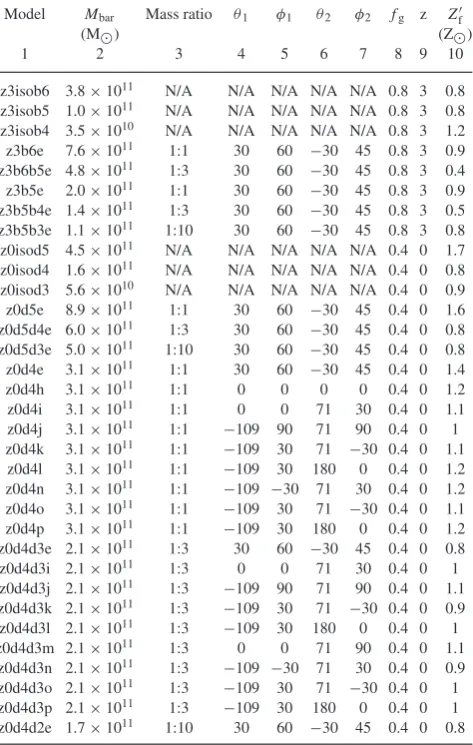
We first require model galaxies to analyse. We simulate the hydro-dynamic evolution of disc galaxies in isolation and galaxy mergers over a range of galaxy masses, merger mass ratios and redshifts utilizing a modified version of the publicly available code,GADGET -2. These simulations provide information regarding the kinematic structure, mass and metal distribution of the ISM, as well as the stellar populations. Table A1 summarizes the model properties.
The remainder of our calculations occur in post-processing. We smooth the smoothed particle hydrodynamic (SPH) results on to an adaptive mesh. We require knowledge of the physical and chemical state of the molecular clouds in our model galaxies. We assume the cold H2 gas is bound in spherical GMCs with H2 fractions
calculated following the models of Krumholz, McKee & Tumlinson (2008) and Krumholz, McKee & Tumlinson (2009a). Carbon is assumed to have a uniform abundance within these clouds of 1.5× 10⁻⁴×Z, whereZ is the metallicity with respect to solar. The
fraction of carbon locked up in CO is determined following the models of Wolfire et al. (2010), and have an explicit dependence on the metallicity. GMCs that have a surface density greater than 100 Mpc−2are considered resolved. GMCs that are not resolved
(typically low-mass GMCs in large cells in the adaptive mesh) have a floor surface density of the aforementioned value imposed, consistent with observations of Local Group GMCs (e.g. Bolatto et al. 2008; Fukui & Kawamura 2010). Unresolved GMCs have velocity dispersions equal to the virial velocity of the GMC, whereas resolved GMCs have velocity dispersions determined directly from the simulations.
The temperature of the GMCs is determined via a balance of the various heating processes on the gas (here, photoelectric effect, cosmic rays and energy exchange with dust), and line cooling. The dust temperature is calculated via the publicly available dust radiative transfer code,SUNRISE(Jonsson, Groves & Cox 2010). The
cosmic ray heating rate is assumed to take on the mean Galactic value (except as described in Appendix C). Utilizing this model, the temperature ranges typically from∼10 K in quiescent GMCs to >100 K in the centres of starbursts (Narayanan et al. 2011b).
Once the physical and chemical state of the ISM is known, we are prepared to model the CO line emission via radiative transfer calculations. The emergent CO line emission from the GMCs is cal-culated via an escape probability formalism (Krumholz & Thomp-son 2007). This radiation is then followed through the galaxy in order to account for radiative transfer processes on galaxy-wide
scales (Narayanan et al. 2006, 2011b). With these calculations, we know the thermal and chemical state of the molecular ISM in our model galaxies, the synthetic broad-band SEDs and the modelled CO emission line spectra. At this point, we are in a position to understand variations in the CO–H2conversion factor. We remind
the reader that further details regarding the implementation of these models can be found in the Appendix.
We note that in order to alleviate confusion between simulation points and observational data on plots, we will employ a system throughout this work in which filled symbols exclusively refer to observational data, and open symbols refer to simulation results.
3 T H E E F F E C T O F G A L AC T I C E N V I R O N M E N T O N XCO
Our general goal is to understand howXCOdepends on the
physi-cal environment in galaxies, and how it may vary with observable properties of galaxies. In order to do this, we must first develop intuition as to how various physical parameters affectXCO. In this
section, we examine howXCOvaries from the Galactic mean in
low-metallicity environments, high-surface density environments and at high redshift.
Quantitatively, we define the meanXCOfrom a galaxy as:
XCO =
H2dA
WCOdA
(4)
which is equivalent to a luminosity-weightedXCOover all GMCs
in the galaxy.
3.1 Review ofXCOinz=0 quiescent disc galaxies
We begin by considering XCO in disc galaxies at z = 0 with
metallicities around solar (Z ≈ 1). These galaxies have mean X-factors comparable to the Galactic mean and will serve as the ‘control’ sample from which we will discuss variations in physical parameters.
Recalling Section 2, and referring to the Appendix, when clouds are not resolved, we impose a floor surface density of 100 Mpc−2.
In these GMCs, the velocity dispersion is the virial velocity of the cloud. In our modelz=0 disc galaxies, gas compressions within the galaxy are unable to cause significant deviations from these subresolution values ofNH2 ∼1022cm−2andσ ∼1−5 km s−1.
In this regime, the temperatures of the GMCs typically fall to∼8– 10 K. This is the usual temperature where cosmic rays dominate gas heating in our model; the densities are not sufficiently high for any of the heating processes to increase the gas temperatures drastically. At∼solar metallicities, a sufficient column of dust can easily build up to protect the CO from photodissocation, and most of the carbon in molecular clouds is in the form of CO. With these modest conditions in the clouds, and little variation throughout the galaxy (see fig. 2 of Narayanan et al. 2011b), the modelledXCO
tends to be ∼ a few×1020 cm−2/K-km s−1(i.e. similar to the
Milky Way mean), with the only notable exception being GMCs towards the galactic centre (Narayanan et al. 2011b).
As pointed out by Narayanan et al. (2011b), while various sub-resolution techniques are folded into our model disc galaxies, that we see relatively little variation in the GMC properties in our model z = 0 discs is a statement that the galactic environment is not extreme enough to cause significant deviations from the default surface densities and velocity dispersions. The temperatures and velocity dispersions are allowed to vary freely with galactic en-vironment, and the surface densities have a floor value similar to
2012 The Authors, MNRAS421,3127–3146
actual GMCs (Blitz et al. 2007; Bolatto et al. 2008). As shown by Shetty et al. (2011a), GMCs with physical parameters comparable to those observed in Galactic GMCs exhibitXCOvalues close to
the Galactic mean, XCO≈ 2–4×1020cm−2/K-kms−1[αCO≈ 3–
6 Mpc−2(K−kms−1)−1]. As we will show, in mergers in the
present Universe, low-metallicity galaxies and, in some cases, high-redshift discs, the physical properties of GMCs vary sufficiently that this is no longer the case.
3.2 The effects of metallicity onXCO
The metallicity of the gas can have a strong effect on the CO–H2
conversion factor. In metal-poor gas, it is possible to have ‘CO-dark’ molecular clouds (Papadopoulos, Thi & Viti 2002; Wolfire et al. 2010). In these regions, H2 can self-shield to protect itself from
photodissociating UV radiation, whereas CO cannot and requires dust to survive (Sternberg & Dalgarno 1995; Hollenbach & Tielens 1999). In these cases, we expect a larger fraction of CO-dark clouds and a rise in the CO–H2conversion factor (Maloney & Black 1988;
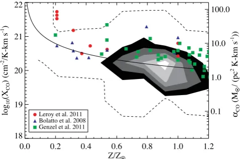
Wolfire et al. 2010; Shetty et al. 2011b; Feldmann et al. 2011). In Fig. 1, we plot the emission-weighted meanXCOfor our model
z=0 isolated disc galaxies as a function of metallicity with filled contours. To control for surface density effects, we plot models with H2≈100 M−2. The contours indicate the number of snapshots in
a givenXCO−Zbin. The outer dashed contour denotes the contour
that encompasses all of our models, at any gas surface density. The lowest metallicity model galaxies all have relatively high meanX-factors compared to the∼solar metallicity galaxies. The lowest metallicity models can have meanX-factors approximately an order of magnitude greater than the Galactic mean. As the galax-ies evolve and the ISM becomes enriched with metals, the carbon is almost exclusively in the form of CO, and theX-factor decreases. The predictedXCO–Zrelation in Fig. 1 matches well with recent
observational data. Overlaid, we plot recent results from resolved regions in nearby galaxies from Bolatto et al. (2008), Leroy et al. (2011) and Genzel et al. (2012). Note thatH2(and thusXCO) in
[image:5.595.44.283.486.644.2]the observations depends on an estimate of the gas mass, which is
Figure 1. XCOversus mass-weighted mean metallicity (in units of solar) for allz=0 model galaxies withH2 ∼100 Mpc−2. The contours represent the number of snapshots in a givenXCO–Zbin, with the numbers increasing with increasing lightness of the contour. The dashed line outer contour encompasses all model galaxies, regardless of their gas surface density. Overlaid are observational data points from Bolatto et al. (2008), Leroy et al. (2011) and Genzel et al. (2012). The solid line shows our best fit to the simulations and is expressed in equation (8) and described in Section 4.
obtained with various methods for these studies.2Both the
obser-vations and models show an upward trend inXCOwith decreasing
metallicity. While we defer a discussion of fittingXCO in terms
ofZto Section 4, we denote our best-fitting model (discussed in equation 8) by the solid line in Fig. 1.
We should note that the contours in Fig. 1 indicate the range of possibleX-factors at a given metallicity as returned by our models. They are not cosmological, and so do not connote any particular probabilities. The simple fact that observed data points lie within the contours with a similarXCO–Ztrend suggests a reasonable match
between our models and observed galaxies. When examining the outer contour that encompasses all of our models (and not just those at a given surface density as in the grey-scale contours), it is clear that there is a significant dispersion inXCOon either side of the
best-fitting line in Fig. 1. Moreover, there is a significant dispersion in the observed data at a given metallicity (especially noticeable near Z≈1). This suggests that there is a second parameter controlling theX-factor in galaxies, aside from metallicity. As we will show in the next section, this is the dynamical and thermal state of the molecular ISM.
3.3 High surface density galaxies
3.3.1 Large temperatures and velocity dispersions
On average, in regions of high surface density, the emission-weighted meanXCOin a galaxy is lower than the Galactic mean
value of∼2–4×1020 cm−2/K-km s−1. This has been shown
ob-servationally by Tacconi et al. (2008), and seen in the models of Narayanan et al. (2011b).
By itself, an increase in surface density does not causeXCOto
decrease. Rather, the opposite is true: per equation (1), at high surface densities,XCOwouldincreaseifWCOwere fixed. However,
in high-H2regions, the velocity-integrated line intensity,WCO, in
fact increases even more rapidly thanH2, causing a net decrease
inXCO. To see why this is the case, consider the physical processes
that are typically associated with increased surface densities. First, regions of high surface density are associated with higher SFRs (Kennicutt 1998a; Krumholz, McKee & Tumlinson 2009b; Ostriker, McKee & Leroy 2010; Ostriker & Shetty 2011). While a variety of theories exist as to why this is the case (see a review of some of these models in Tan 2010), in our simulations this is due to the fact that we explicitly tie our SFRs to the volumetric gas density on small scales. With high SFRs come hotter dust tem-peratures as the UV radiation heats the nearby dust grains. When the gas densities are104cm−3, the dust and gas exchange energy
efficiently, and the gas temperature approaches the dust tempera-ture (Goldsmith 2001; Juvela & Ysard 2011). Hence, in regions of high surface density, the increased dust temperature driven by the higher SFRs causes an increase in the gas kinetic temperature. Because the CO (J=1-0) line is thermalized at relatively low den-sities, the brightness temperature of the line is comparable to the kinetic temperature of the gas, and is thus increased in regions of
2Bolatto et al. (2008) assume clouds are virialized; if instead clouds are marginally bound, thenXCOwould decrease. Leroy et al. (2011) use infrared emission to derive dust masses, and HIobservations to derive a dust-to-gas ratio. If this dust-to-gas ratio does not map to the H2gas, the derivedXCO will change accordingly. Genzel et al. (2010) assume a scaling relation
SFR ∝1gas.1. If a steeper relation were adopted (cf. Section 4.2), then the values ofXCO corresponding to high values ofSFRwould decrease somewhat.
2012 The Authors, MNRAS421,3127–3146
high surface density. For low-redshift galaxies, the easiest way to increase the surface density tends to be through merging activity and the associated tidal torques which drive gaseous inflows into the nuclear region (Barnes & Hernquist 1991, 1996; Mihos & Hern-quist 1994b, 1996), though higher-redshift discs can have relatively large surface densities simply due to gravitational instabilities in extremely gas-rich clumps (Springel, Di Matteo & Hernquist 2005; Bournaud et al. 2010).
Secondly, in the simulations, high surface densities in gas are typically accompanied by high velocity dispersions. This generally means some level of merging activity in low-redshift galaxies, and either merging activity or unstable gas clumps in high-redshift discs. In major mergers, the emission-weighted velocity dispersions can be as high as∼50–100 km s−1.
The increased velocity dispersion and kinetic temperature con-tribute roughly equally to increasing the velocity-integrated line intensity. During a merger, the temperature and velocity dispersion individually increase enough to offset the increase in the gas sur-face density, and in combination tend to drive the emission-weighted meanXCOfor a galaxy below the Milky Way average. In regions
of high surface density, the emission-weighted meanXCOtends to
decrease on average. In Section 3.4, we detail specific numbers for a sample merger that serves as an example for this effect.
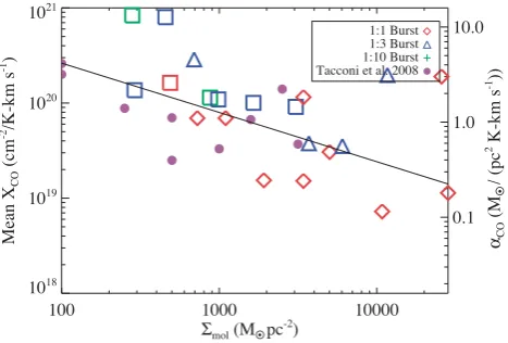
We can see this more explicitly in Fig. 2, where we plot the mean XCOversus mean surface density for the starburst snapshots in our
low-redshift sample of galaxies. The starburst snapshots are defined as the snapshots where the SFR peaks for a given model and are categorized by the merger mass ratio (1:1, 1:3 and 1:10). The mean surface density is defined as the mass-weighted surface density over all GMCs,i, in the galaxy:
H2 =
iH2,i×MH2,i
iMH2,i
(5)
Henceforth, when we refer to the surface density of the galaxy, we refer to the mean surface density defined by equation (5). We note that this is different from the commonly used definitionH2 =
MH2/A, whereAis the area within an observational aperture. We
[image:6.595.310.545.56.219.2]refrain from the latter definition as it is dependent on the choice of
[image:6.595.50.284.499.657.2]Figure 2. MeanXCOversus mass-weighted mean surface density forz=0 model mergers when they are undergoing a starburst (e.g. the snapshots with the peak SFRs). The plotting symbols are shown in the legend, though a given symbol may be replaced by a square if the metallicity is lower than 0.5Z. The purple filled circles represent the compiled data from Tacconi et al. (2008). The black solid line is the best fit for all simulation snapshots from equation (10), and is discussed in Section 4.
Figure 3. XCOversus CO line intensity,WCOforz=0 1:1 galaxy mergers in two distinct metallicity bins. In this case,WCOis a surrogate forH2that is an actual observable (and relatable viaXCO). At a given metallicity,XCO decreases with CO intensity due to the larger number of CO-dark GMCs in these galaxies. The solid line shows the best-fitting model (cf. Section 4) for a metallicity ofZ=1.
scale.H2 can be thought of as the surface density at which most
of the mass resides. Immediately, we see two trends in Fig. 2. First, with increasing surface density, we see decreasing mean XCOdue to the warm and high velocity dispersion gas associated
with merging systems. Secondly, the most violent mergers tend to have the lowest mean XCO values, whereas lower mass ratio
mergers (1:3) have less extreme conditions, and thusX-factors more comparable to the Galactic mean value. The purple circles in Fig. 2 note observational points from Tacconi et al. (2008); the models and data show broad agreement.3
The open squares in Fig. 2 are points from our models with mean metallicities less thanZ<0.5. Careful examination of these points shows that some of them have rather largeX-factors. As we discussed in Section 3.2, lower metallicity galaxies have larger mass fractions of CO-dark clouds, and thus higherX-factors.
In Fig. 3, we demonstrate more explicitly the effect of metallicity on theXCO–surface density relationship. Because we find it useful in
a forthcoming section (Section 4) to parametrizeXCOin terms of the
observable velocity-integrated CO intensity,WCOas an observable,
rather thanH2, we plotXCOagainstWCOin Fig. 3.WCOis defined
as the luminosity-weighted line intensity from all GMCs in the galaxy. We plot theXCO–WCOrelationship for all snapshots of all
1:1 z= 0 major mergers within two distinct metallicity ranges. The selected metallicity ranges are arbitrary, and are chosen simply to highlight the influence of metallicity. As is clear, the lowest metallicity points in Fig. 3 have the highest X-factors, and the reverse is true for the highest metallicity points. For each metallicity bin, the trend is such that increasingWCO(orH2) correlates with
decreasingXCO, though the normalization varies with metallicity.
This informs our fitting formula in Section 4.
Returning to Fig. 2, we make a final point that there is a large dis-persion inXCOfor the merger models. Both the 1:3 models and 1:1
3We caution that our definition of
H2 is a mass-weighted surface den-sity, and is different from the surface density defined by the Tacconi et al. data,MH2/A. In the limit of a large volume filling factor, these values will approach one another. The observed data closer tomol=100 Mpc−2 likely represent galaxies with a clumpy ISM, and the modelled and observed H2gas surface densities may differ in this regime.
2012 The Authors, MNRAS421,3127–3146
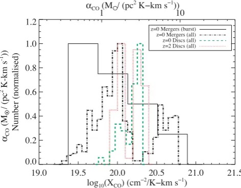
Figure 4. Distribution ofXCOvalues during the peak of the SFR (the ‘burst’ snapshot) for all 1:1 and 1:3 local galaxy mergers (black solid), allz=0 1:1 and 1:3 mergers (i.e. not just the burst snapshots; black dash-dot), all high-z
disc models withZ≈1 (red dotted) and low-zdisc models withZ ≈1 (green dashed). See text for details.
mergers showXCOvalues ranging from above the Milky Way mean
to an order of magnitude below it during their peak starburst. When sampling the entire library of merger orbits for a given merger mass ratio, a wide range in outcomes is apparent. We see a diverse set of velocity dispersions in the gas, as well as SFRs, owing to differ-ing efficiencies at which angular momentum is removed from the gas. Some models undergo rather vigorous starbursts (approach-ing ∼500 Myr−1), whereas others hardly sustain a noticeable
starburst upon final coalescence. Galaxies that undergo their peak starburst only on first passage can have rather different metallicities in their ISM than mergers that go through a vigorous star forma-tion period during first passage and inspiral before experiencing a starburst contemporaneous with final coalescence.
In the solid line of Fig. 4, we plot the distribution of emission-weighted meanXCOvalues for each of our 1:1z=0 merger models
during the peak of their SFR. For comparison, we plot the distribu-tion ofX-factors for ourz=0 discs in the green dashed line (only plotting galaxies with∼solar metallicity), as well as the distribution ofXCOfor ourz=2 discs (which we discuss in more detail in
Sec-tion 3.4). As we see, there is no ‘merger’ value forXCO. It is possible
to haveXCOvalues in starbursting mergers comparable to the Milky
Way’s. The fact that starbursting mergers, on average, have lower X-factors than the Galactic mean is likely due to a selection effect. We return to this point in more (quantitative) detail in Section 4.
3.4 XCOin high-redshift galaxies 3.4.1 Basic results
Now that we have developed intuition regarding the variation of XCO with metallicity and surface density, we are in a position to
understand how galaxies at high redshift may behave with respect to the CO–H2conversion factor.
Mergers at highzare some of the most luminous, rapidly star-forming galaxies in the Universe. As an example, many z ∼ 2 submillimetre-selected galaxies (SMG) form stars at 1000 M yr−1 (Narayanan et al. 2010a). However, despite the ∼order of
magnitude greater SFR in these galaxies compared to local mergers,
mergers at highzare similar to their low-redshift counterparts in terms of their typicalX-factors. While the mean gas surface densities in e.g.z∼2 SMGs are larger than low-redshift mergers (e.g. Tacconi et al. 2008; Narayanan et al. 2010a), both the dust temperatures and gas velocity dispersions also rise commensurately.
As a specific example, we focus on a 1:1 major merger atz∼2 (This is model ‘z3b5e’; please refer to Table A1 in the Appendix for the initial conditions of this model merger.). Model z3b5e undergoes a luminous burst of∼1500 Myr−1, and may be selected as a
SMG when it merges (Narayanan et al. 2009; Hayward et al. 2011). During the burst, this simulation reaches a mass-weighted mean surface density of molecular gas of∼104M
pc−2. At the same
time, the mass weighted kinetic(dust) temperature is∼150(160) K,4
and the mass-weighted velocity dispersion in the GMCs is∼140 km s−1. Doing a simple scaling results in a meanX
COof∼5×10¹⁹
cm−2/K-km s−1. Of course, the real mass-weighted value may vary
from this owing to both radiative transfer as well as the fact that this simple scaling is not a true averaging. Observational estimates of theX-factor in SMGs suggest that they are similar to the lower values in the range of local ULIRGs (Tacconi et al. 2008).
Our simulated disc galaxies at high-redshift show a range ofXCO
values, ranging from comparable to the Galactic mean to values two to five times lower. The reason massive discs at high-redshift may have lowerX-factors than the Galactic mean can be understood in the following way. In contrast to present-epoch galaxies, galaxies at higher-redshifts (z1) at a fixed stellar mass are denser and more gas-rich (e.g. Erb et al. 2006; F¨orster Schreiber et al. 2009; Daddi et al. 2010b; Tacconi et al. 2010). Both simulations and observations suggest that galaxies around redshiftsz∼1–2 may have baryonic gas fractions of order 20–60 per cent (Dav´e et al. 2010; Daddi et al. 2010b; Tacconi et al. 2010). A primary consequence of this is that discs at higher-redshifts may be heavily star forming, with SFRs of the order of∼102M
yr−1, comparable to local galaxy mergers
(Daddi et al. 2007; F¨orster Schreiber et al. 2009; Narayanan et al. 2010b). In fact, simulations suggest that disc galaxies atz∼2 likely dominate the infrared luminosity function (Hopkins et al. 2010).
In the absence of rather extreme stellar feedback, very gas rich discs at high redshift can be unstable to fragmentation, and form massive∼kpc-scale clumps (e.g. Springel et al. 2005; Ceverino, Dekel & Bournaud 2010). These clumps can have relatively high velocity dispersions (∼102 km s−1) and warm gas temperatures
owing to high volumetric densities and high SFRs (Bournaud et al. 2010).
These effects are the strongest in the most massive discs. Our most massivez=2 model disc galaxy has a total baryonic mass of ∼5×10¹¹M
yr−1, and has typical5X-factors ranging anywhere
between a factor of 5 below the Galactic mean to the Galactic mean value. The lower massz= 2 isolated disc models (with baryonic masses ofMbar= 1×10¹¹ and 3.5×10¹⁰ M) typically have
4Note that owing to radiative transfer effects, this dust temperature is not necessarily what would be derived simply by identifying the location of the peak of the SED.
5Because our simulations are not cosmological, there is no accretion of intergalactic gas. As a result, the metallicities in our model galaxies only rise with time. Because theX-factor is dependent on metallicity (Section 3.2), we have to make a choice as to which snapshot/metallicity to consider as a ‘typical’ galaxy. We assume any snapshot aboveZ > 0.5 is ‘typical’ based on the steady-state metallicities found for galaxies of baryonic mass comparable to those in our sample from cosmological modelling (fig. 2 of Dav´e et al. 2010, though see Keres et al. 2011; Vogelsberger et al. 2011 and Sijacki et al. 2011).
2012 The Authors, MNRAS421,3127–3146
X-factors comparable to the Milky Way mean. Returning to Fig. 4, we examine the red dotted line that representsz∼2 disc models. Because the idea of a ‘starburst’ snapshot is less meaningful for the evolution of a disc galaxy, we plot theX-factor for every snapshot for our model discs with metallicities around solar. We see a large spread in meanX-factors.
3.4.2 Do mergers and discs have inherently different X-factors?
In light of the fact that high-z discs have, at times, SFRs com-parable to local galaxy mergers, a pertinent question is whether there is an intrinsic difference in theX-factor between high-zdiscs and galaxy mergers. Another way of saying this is, for a given set of physical conditions, are theX-factors from mergers lower than theX-factors from high-zgas-rich, gravitationally unstable discs? A cursory examination of Fig. 4 indicates that mergers (the black solid line) have systematically lowerX-factors than discs (the blue and red dashed and dotted lines). Indeed, in the local Universe, it is observed that mergers have, on average, lowerX-factors than discs (e.g. Tacconi et al. 2008). However, this is likely due to a selection bias. We remind the reader that the black solid line in Fig. 4 rep-resentsstarburstingmergers. These mergers are caught when their gas is extremely warm and with large velocity dispersion. When comparing mergers and discs with comparable physical conditions, the observedXCOvalues are in fact quite similar. It is the physical
conditions in a galaxy that determine theX-factor, not the global morphology.
To demonstrate this, we perform three tests. First, we compute the distribution ofXCOvalues forall1:1 and 1:3 merger snapshots
(at∼solar metallicity), and indicate this with the black dot–dashed line in Fig. 4. As we see, the distribution ofXCOvalues is broad, but
with substantially less power in the lowX-factor regime than the distribution that denotes only starbursting mergers (black solid line). This highlights that mergers which are selected during a particularly active phase are more likely to have lowX-factors, due to their warm and high-σgas. When controlling for this effect by picking galaxies with similar CO intensity (WCO) and metallicity, mergers and discs
have the sameXCOon average.
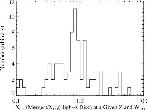
To show this, in Fig. 5, we perform our second test in which we examine the X-factors from all the 1:1 and 1:3 mergers (at lowz) and compare them to theXCOfrom high-zdiscs with the
same6metallicity and CO intensity (W
CO). We could equivalently
perform this analysis in terms ofH2, though as we will show in
Section 4, parametrizing in terms ofWCOis desirable with regard
to observations. There is a strong peak atXCO ratios near unity,
with some spread. The median value in the distribution is∼0.8, and the mean is∼1.1. The implication from Fig. 5 is that galaxies with similar physical conditions (hereZ and WCO) have similar
X-factors, regardless of whether they are discs or mergers. The fact that mergers, on average, have lowerX-factors than discs in the local Universe likely derives from the fact that they are selected as starbursts, which have preferentially higher temperatures and velocity dispersions in the gas.
Thirdly, in Fig. 6, we examine the relationship betweenXCOand
WCOfor the same galaxies plotted7in Figs 4 and 5. These are all
galaxies with metallicities around solar. The principal result from
6‘The same’ here means that the values ofZandWCOare within 10 per
cent of one another.
[image:8.595.310.546.57.233.2]7To reduce clutter in the plot, we randomly draw 10 per cent of the galaxies within each merger ratio bin to plot.
[image:8.595.311.548.339.508.2]Figure 5. Comparison of theX-factor between low-zmergers (1:1 and 1:3) and high-zstar-forming discs. The histogram denotes the ratio ofX-factor from mergers versus high-zdiscs between snapshots with a similar metal-licity and CO intensity. The sharp peak near unity implies that galaxies with similar physical conditions have similarX-factors, independent of large-scale morphology.
Figure 6. Comparison ofXCOversus CO intensity (WCO) for low-zgalaxy mergers and high-zdiscs in an effort to investigate if mergers and discs inherently have differentXCO properties. Included in this plot are all 1:1 and 1:3 mergers simulated atz= 0. Only snapshots with metallicitiesZ>
0.7 are shown. To reduce clutter in the plot, we plot only a randomly drawn subsample (10 per cent) of the snapshots from each mass ratio. The line shows the best fit from equation (8). Evidently, galaxies that have similar physical conditions have similarX-factors, independent of galaxy morphology or evolutionary history. See text for details.
Fig. 6 is that galaxies within a relatively limited metallicity andWCO
(or surface-density) range have similarX-factors, regardless of the type of merger it is. Mergers and discs have similarXCO values
when they have similar physical conditions, and are not inherently different based on their global morphology. In addition, Fig. 6, like Figs 2 and 3, shows a systematic decrease ofXCOwith increasing
WCO(andmol).
2012 The Authors, MNRAS421,3127–3146
4 A P P L I C AT I O N T O O B S E RVAT I O N S 4.1 DerivingXCOfrom observations
As we have seen from the previous sections, it is clear that there is a continuum ofXCOvalues that vary with galactic environment. The
dominant drivers of theX-factor in our simulations are the metallic-ity of the star-forming gas, and the thermal and dynamical state of the GMCs. Informed by this, we are motivated to parametrizeXCO
as a function of observable properties of galaxies.
Metallicity is a crucial ingredient to any parametrization. At sub-solar metallicities, we see the rapid growth of CO-dark GMCs. This has been noted both in observations (e.g. Leroy et al. 2011; Genzel et al. 2012) and in other numerical models (Feldmann, Gnedin & Kravtsov 2011; Krumholz, Leroy & McKee 2011; Shetty et al. 2011b). As we saw in Section 3.2, as well as in Fig. 3, at a given galaxy surface density (or CO intensity),XCOincreases with
decreasing metallicity.
Beyond this, as was shown in Section 3.3, as well as in the models of Narayanan et al. (2011b), galaxy surface density is correlated with the thermal and dynamical state of the gas: at a given metallicity, higher surface density galaxies, on average, correspond to galaxies with a warm and high velocity dispersion molecular ISM, due to their higher SFRs.
Informed by these results, we perform a 2D Levenberg– Marquardt fit (Markwardt 2009) on our model galaxies (consid-ering every snapshot of every model), fittingXCOas a function of
mass-weighted mean metallicity and mass-weighted mean H2
sur-face density. We find that our simulation results are reasonably well fitted by a function of the form:
XCO≈
1.3×10²¹
Z× H2 0.5 (6)
whereH2is in units of Mpc−2andXCOis in units of cm−2
/K-km s−1. Equation (6) provides a good fit to the model results above
metallicities ofZ ≈0.2. Turning again to Figs 1, 2, 3 and 6, we highlight the solid lines which show how equation (6) fits both the simulation results and observational data. We note that Ostriker & Shetty (2011) obtained a similar result,αCO∝mol−0.5, by
interpolat-ing between empiricalαCOvalues (αCO=3.2 formol=100 M
pc−2andα
CO=1 formol=1000 Mpc−2).
BecauseH2is not directly observable (hence the need for anX
-factor), we re-cast equation (6) in terms of the velocity-integrated CO line intensity. In order to parametrize XCO in a manner that
is independent of the effects of varying beam-sizes or observa-tional sensitivity, we define the observable CO line intensity as the luminosity-weighted CO intensity over all GMCs,i:
WCO =
W2
COdA
WCOdA
≡
LCO,i×WCO,i
LCO,i
(7)
whereWCO is in units of K-km s−1, and is the CO surface
bright-ness of the galaxy. We then fit to obtain a relation betweenXCO,Z
andWCO :
XCO=
6.75×10²⁰× W CO −0.32
Z0.65 (8)
where againWCO is CO line intensity measured in K-km s−1,
XCOis in cm−2/K-km s−1andZ is the metallicity divided by the
solar metallicity. By convertingXCOtoαCO, we similarly obtain:
αCO=
10.7× WCO −0.32
Z0.65 (9)
whereαCOis in units of Mpc−2(K-km s−1)−1.
It is important to recognize that the power law in equation (8) cannot describeXCOindefinitely. At very low WCO, GMCs tend
towards fixed properties in galaxies and the galactic environment plays a limited role in settingXCO. Considering this, equation (8)
formally becomes
XCO=
min4,6.75× WCO −0.32
×1020
Z0.65 (10)
or, similarly:
αCO=
min6.3,10.7× WCO−0.32
Z0.65 . (11)
Equations (10) and (11) can be used directly with observations of galaxies to infer an expectedX-factor. One advantage of this formalism is that it captures the continuum of CO–H2conversion
factors, rather than utilizing bimodal ‘disc’ and ‘ULIRG’ values. Because we have chosen the physical quantities in our modelling based on mass or luminosity-weighted averages, they are defined without reference to a particular scale. Consequently, equation (10) can be used on scales ranging from our resolution limit of∼70 pc to unresolved observations of galaxies.
It is conceivable that alternative definitions of the observed mean CO intensity could be appropriate. One can imagine implement-ing an area-weighted intensity, i.e.WCO=LCO/Area. This has the
undesirable attribute of being dependent on a defined scale.
4.2 The Kennicutt–Schmidt star formation relation in galaxies fromz= 0 to 2
A natural application of our model for the CO–H2conversion factor
is the KS SFR surface density–gas surface density relation in galax-ies. Because the inferred H2gas masses from observed galaxies
are inherently dependent on conversions from CO line intensities, our understanding of the KS relation is fundamentally tied to the potential variation ofXCOwith the physical environment in galaxies.
Recent surveys of both local galaxies (e.g. Kennicutt 1998a,b; Bigiel et al. 2008, and references therein) and pioneering efforts at higher redshifts (e.g. Bouch´e et al. 2007; Bothwell et al. 2010; Daddi et al. 2010a; Genzel et al. 2010) have provided a wealth of data contributing to our knowledge of the star formation relation in both quiescent disc galaxies and starbursts. Work by Daddi et al. (2010a) and Genzel et al. (2010) demonstrate the sensitivity of these relations to the CO–H2conversion factor: when applying the
traditional bimodal conversion factor (XCO≈8×1019cm−2/K-km
s−1for ULIRGs andX
CO≈2×1020cm−2/K-km s−1for discs) to
the starburst galaxies and discs, respectively, a bimodal SFR relation becomes apparent when the data are plotted in terms ofSFRand
mol.
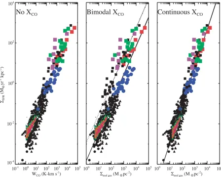
In Figs 7–9, we illustrate the effects of our model fit forXCO
as a function of galaxy physical properties. In the left-hand panel of Fig. 7, we plot the SFR surface density for both local galaxies and high-zgalaxies as compiled by Daddi et al. (2010a) and Genzel et al. (2010) against their CO line intensity,WCO. Although there is
significant scatter, theSFRversusWCOrelation is unimodal. In the
middle panel, we plot the SFR–H2relation utilizing the bimodal
X-factors assumed in the literature [with the above ‘ULIRG’ value for the inferred mergers (local ULIRGs and high-zSMGs), and the above ‘quiescent’ value for low-zdiscs and high-z BzKgalaxies].8
8In practice, for the high-z BzKgalaxies, we utilize anX-factor ofX CO≈ 2.3×1020cm−2/K-km s−1to remain consistent with Daddi et al. (2010a), though the usage of this versus the more standard disc value makes little difference.
2012 The Authors, MNRAS421,3127–3146
Figure 7.KS star formation relation (SFR surface density versus H2gas surface density) in observed galaxies. Circles and triangles are local discs or high-z BzKgalaxies, and squares are inferred mergers (local ULIRGs or high-zSMGs). Colours denoting separate surveys are described below. Left: SFR surface density versus velocity-integrated CO intensity, yielding a unimodal SFR relation. Centre: when applying an effectively bimodalXCO(αCO=4.5 for local discs, 3.6 for high-zdiscs and 0.8 for mergers), the resulting SFR relation is bimodal. The solid and dotted lines overplotted are the best-fitting tracks for each ‘mode’ of star formation as in Daddi et al. (2010a). Right: SFR relation when applying equation (10) to the observational data, resulting in a unimodal SFR relation. The power-law index in the relation is approximately 2 (solid line). Symbol legend: we divide galaxies into ‘disc-like’ with filled circles, and ‘merger-like’ with squares. This assumes that high-z BzKgalaxies are all discs, high-zSMGs and low-zULIRGs are all mergers. The low-zdisc observations (black filled circles and black triangles) come from Kennicutt et al. (2007), Wong & Blitz (2002), Crosthwaite & Turner (2007), Schuster et al. (2007) and comprise both resolved and unresolved points. The resolved points from the survey of Bigiel et al. (2008) are denoted by the coloured contours. The local ULIRGs are compiled by Kennicutt (1998b) and are denoted by black filled squares. The high-zdiscs come from Genzel et al. (2010), Daddi et al. (2010a,b) and are represented by filled blue circles. The high-zSMGs are divided into the samples of Bothwell et al. (2010) (purple), Bouch´e et al. (2007) (green) and Greve et al. (2005), Tacconi et al. (2006; 2008), Engel et al. (2010) as compiled by Genzel et al. (2010) (filled red squares).
The circles are unresolved observations of disc galaxies at low and high z, triangles and contours are resolved observations of local discs, and the squares are local ULIRGs and inferred mergers at high-redshift. When separate high and low values ofXCO are
adopted for discs and mergers, a bimodal relationship betweenSFR
andgasresults, with power-law index ranging between unity and
1.5.
In the right-hand panel of Fig. 7, we apply equation (10) to the observational data (assumingZ=1 for the galaxies). The scatter in the modified relation immediately tightens, and it becomes uni-modal. To numerically quantify the reduction in scatter with the modified relation we examine the ratio of the maximum inferred H2to the minimum for all points within the relatively tight SFR
surface density range of [0.05,0.1] Myr−1kpc−2for the centre and
right-hand panels of Fig. 7. The scatter is reduced by approximately
a factor of 5. Within thisSFRrange, no mergers are in the sample.
Thus, the reduction in scatter is not due to simply using a unimodal XCOversus bimodalXCO. We note that in applying equation (10) to
the observed data, we have to assume that the intensity within the reported area is uniform. If the emission is instead highly concen-trated over very few pixels, then the application of equation (10) may overestimateXCO.
The reason for the transition from a bimodal to unimodal KS relation is clear. In the modified relation, similar to the traditional KS plot that uses a bimodalX-factor, the lower luminosity discs have CO–H2conversion factors comparable to the Galactic mean,
and the most luminous discs haveX-factors up to an order of magni-tude lower. Very massive, gas-rich, unstable discs, as well as lower luminosity mergers, haveX-factors in between the two, however, and fill in the continuum. Utilizing equation (10), a simple linear
2012 The Authors, MNRAS421,3127–3146
Figure 8. Similar to Fig. 7, but with the abscissa showingWCOormoldivided by the orbital time of the observed galaxy. Symbols are the same as in Fig. 7, but we omit galaxies for which orbital times are not available. The best-fitting slope in the right-hand panel is of the order of unity. See text for details.
chi-square fit of the observed data on the right-hand side of Fig. 7 returns:
log10(SFR)=1.95×log10(mol)−4.9 (12)
whereSFRis measured in Myr−1kpc−2andmolis measured in
Mpc−2. Utilizing an empirical method to obtainX
CO∝WCO−0.3,
Ostriker & Shetty (2011) previously showed that the observational data compiled in Genzel et al. (2010) yield a similar fit to equa-tion (12).
We remind the reader of the assumptions that have gone into this fit: we have assumed that every galaxy has solar metallicity, and neglected any potential effects of differential excitation in the CO as a function of infrared luminosity (e.g. Narayanan et al. 2011a). Nevertheless, the application of a variableX-factor on the SFR–gas surface density relation has interesting implications.
First, the index of∼2 of equation (12) is consistent with the analytic models and hydrodynamic simulations of self-regulated star formation by Ostriker & Shetty (2011). This work suggests that in molecular regions where supernova-driven turbulence controls the SFR and gas dominates the vertical gravity, the SFR surface density should be proportional to the gas surface density squared: log(SFR)=2×log(mol)−5.0 [adopting fiducial parameters in
equation (13) of Ostriker & Shetty (2011)]. This is shown as the solid line in the right-hand panel of Fig. 7, and is very comparable to the best-fitting relation. Secondly, comparing equation (12) to
equation (13) of Ostriker & Shetty (2011), the empirical results are consistent with a value of momentum injected/total stellar mass formed offp×p∗/m∗∼3000 kms−1(mol/100 Mpc−2)−0.05; the
fiducial value adopted in Ostriker & Shetty (2011) is 3000 km s−1.
Daddi et al. (2010a) and Genzel et al. (2010) suggest an alternative mechanism for reducing the scatter imposed by the utilization of a bimodalXCO in Fig. 7. Specifically, these authors find that by
dividing the molecular gas surface density by the galaxy’s orbital time, the observed KS relation goes from bimodal to unimodal, suggesting that the galaxy’s global properties are related to the local, small-scale processes of star formation. That is to say, when using a bimodalXCO, the SFR − mol relationship is bimodal,
whereas theSFR−mol/tdynrelationship is unimodal, with some
scatter.
If one abandons the bimodal XCO approximation, and utilizes
our favoured model for XCO, the observed relationship between
SFRandmol/tdynremains unimodal, and in fact the scatter in the
relation is reduced compared to what one obtains using a bimodal XCO. To show this, in Fig. 8, we show the analogue to Fig. 7, but
with the abscissa showing the surface density orWCOdivided by the
dynamical time. The dynamical times used are the same as those in Daddi et al. (2010a) and Genzel et al. (2010), and are defined as the rotational time at either the galaxy’s outer radius, or half-light radius, depending on the sample. In the left-hand panel of Fig. 8, we show the relationship betweenSFR and WCO/tdyn (i.e. pure
2012 The Authors, MNRAS421,3127–3146
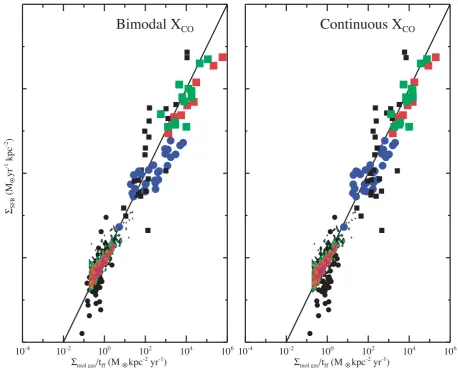
Figure 9. Same as Fig. 7, but instead of plotting/tdynon the abscissa we instead plot/tff, wheretffis the free-fall time in the star-forming clouds of a galaxy – see main text for details. We do not include aSFR−WCO/tffplot as the calculation oftffrequires a gas mass. Symbols are the same as in Figs 7 and 8. The left-hand panel shows the results using a bimodalXCO, while the right-hand panel shows the results using our continuousXCO. The solid black lines show the relationSFR=ffmol/tffwithff=0.01.
observables); in the centre panel, we show the relationship between SFRandmol/tdynwhen assuming a bimodalXCO[as is done in
Daddi et al. (2010a) and Genzel et al. (2010)] and in the right-hand panel we show the same relationship, but withmol determined
using our best-fitting continuousXCO, rather than the bimodalXCO
value used in Daddi et al. (2010a) and Genzel et al. (2010). We find a best-fitting relation (using our model forXCO) of
log10(SFR)=1.03×log10(mol/tdyn)−1.05 (13)
whereSFRandmol/tdynare both in Myr−1kpc−2.
Our best-fittingSFR–mol/tdynrelation has a slope of
approxi-mately unity, comparable to what is found by Genzel et al. (2010), and consistent with the best-fitting slope of Daddi et al. (2010a) of ∼1.15. A principal difference between using our modelXCO
ver-sus the bimodalXCOin calculating theSFR–mol/tdynrelation is a
reduction of scatter. When measuring the scatter near SFR surface density of 1 M yr−1kpc−2, we find that using our modelX
CO
versus the bimodal value reduces the scatter by a factor of∼5. The fact that our model for theSFR–mol/tdynrelation is
con-sistent with the observed one (though with reduced scatter) is not surprising. Daddi et al. (2010a) and Genzel et al. (2010) assume a Milky Way likeXCOfor their disc galaxies, and roughly a
fac-tor of 5 lower for their mergers. In our model, the assumption of a bimodalXCO for discs and mergers is correct on average. The
mean value forXCOfor high-zSMGs and low-zmergers is in fact
lower than the mean value for local discs (cf. Section 4.3). How-ever, many galaxies lie in the overlap region. Some local ULIRGs haveX-factors comparable to the Galactic average, and some high-z discs haveX-factors more similar to the canonical literature ‘merger value’. By modelling the continuous nature ofXCOand more
prop-erly treating these intermediate cases, a reduction in scatter is natural.
Finally, we considerSFRas a function ofmol/tff, wheretffis
the free-fall time within the dense molecular star-forming clouds in the galaxy. Both observations and theory have suggested that the star formation efficiency per free-fall timeffin molecular gas is
approximately constant (Krumholz & McKee 2005; Krumholz & Tan 2007; Evans et al. 2009; Ostriker & Shetty 2011; Krumholz, Dekel & McKee 2012). We infertfffrom the observable properties
of the galaxy (using the approximations of Krumholz et al. 2012), together with either a bimodal XCO or our favoured continuous
XCO. Krumholz et al. show that usingtff rather thantdynmakes it
possible to fit the unresolved extragalactic observations, the resolved observations of Local Group galaxies from Bigiel et al. (2008) and
2012 The Authors, MNRAS421,3127–3146
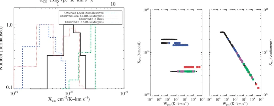
Figure 10. Left: we utilize our model fit forXCO(equation 10) to infer theXCOvalues for observed galaxies compiled by Genzel et al. (2010) and Daddi et al. (2010a). Right: CO line intensity,WCOversusXCOfor the observed galaxies from Fig. 7 (the colour coding of the points is the same as in Fig. 7). TheXCO values are both the original literature values [denoted by ‘XCO(bimodal)’] and our derived values [denoted by ‘XCO(continuous)’].
individual molecular clouds in the Milky Way on a single relation, as illustrated in the left-hand panel of Fig. 9. The right-hand panel of the figure shows that this remains true for our favouredXCO and
that a star formation lawSFR=ffmol/tffwithff≈0.01 remains
a good fit to the observational data. As with theSFR–mol/tdyn
relation, using our continuous XCO actually reduces the scatter,
and for the same reason: our favoured XCOproduces essentially
the same result as the traditional bimodalXCOfor galaxies at the
extremes of the disc and merger sequences, but makes the behaviour ofXCOcontinuous rather than discontinuous for the large number
of galaxies in the overlap region.
The results from Fig. 9 are compatible with the model of Ostriker & Shetty (2011). For a disc in vertical hydrostatic equilibrium with gravity dominated by the gas, and vertical velocity dispersion,vz,
SFR=ffSFR/tff=ff×4Gmol2 /(
√
3vz) (14)
(Ostriker & Shetty 2011, equation 21). Comparing to the fit obtained in equation (12) using our continuous XCO relation, we find that
ff/vz=0.001(kms−1)−1(mol/100 Mpc−2)−0.05. Ifvz≈10 kms−1 on small scales in the dense neutral gas, as suggested by Ostriker & Shetty (2011), this impliesff ≈ 0.01, the value proposed by
Krumholz & McKee (2005) and Krumholz & Tan (2007) and found in Fig. 9. In the self-regulation theory of Ostriker & Shetty (2011), vz/ff∼(1/3)fp×p∗/m∗, so thatvzandffvary together for a given
momentum feedback level.
4.3 Observational constraints on the model andXCOvalues for
observed galaxies
In order to assess the validity of our parametrization ofXCO
(equa-tion 10), it is worth comparing our models to the existing observa-tional constraints in the literature.
As discussed in Section 1, galaxy mergers at low redshift appear to have a range ofXCOvalues, from roughly an order of magnitude
below the Galactic mean to comparable to the Milky Way average (Solomon et al. 1997; Downes & Solomon 1998; Bryant & Scov-ille 1999), though on average theX-factor from local ULIRGs is observed to be below the Galactic mean (Tacconi et al. 2008). At higher redshifts, the constraints onXCOfrom inferred mergers
(typ-ically submillimetre-selected galaxies) come from either dynamical
mass modelling (Tacconi et al. 2008), or dust to gas ratio arguments (Magdis et al. 2011). The inferredX-factors from high-zSMGs also appear to be lower than the Galactic mean by a factor of∼5.
There are relatively fewer constraints onXCOfrom high-zdiscs.
Daddi et al. (2010b) estimated the dynamical masses for resolved CO observations of high-z BzKdisc galaxies. After subtracting off the measured stellar and assumed dark matter masses, they were able to derive anXCOfactor by relating the remaining (presumably
H2) mass to the observed CO luminosity. This method recovered a
meanX-factor∼2×1020cm−2/K-km s−1. This is consistent with
the calculation ofXCOvia dust to gas ratio arguments for a different
BzKgalaxy by Magdis et al. (2011).
In order to investigate how our inferredX-factors for observed galaxies (utilizing our model fit) compare to these determinations, on the left-hand side of Fig. 10, we apply equation (10) to the observed data from Fig. 7, and plot the derivedXCOfor observed
galaxies, binning separately for local ULIRGs, inferredz∼2 discs, and inferredz∼2 mergers. First, as a consistency check, we ex-amine the inferredX-factors employing equation (10) from local disc observations, and denote this by the green dash–dotted line in Fig. 10. As expected, the derivedX-factors from local discs form a relatively tight distribution around the Galactic mean value of 2–4× 1020cm−2/K-kms−1.
From Fig. 10, it is evident that observed SMGs have extremely lowX-factors, with the bulk of them a factor of a few lower than the Galactic mean value. Observed ULIRGs show a large population of galaxies with lowerXCOvalues, with a few approaching the Galactic
mean. This is reasonably consistent with the range of values reported by Solomon et al. (1997), Downes & Solomon (1998) and Bryant & Scoville (1999).
As mentioned, there are far fewer constraints onXCOfrom
high-z discs, with the only constraints placing theX-factors near the Galactic mean value. The values for some of the observed galaxies in Fig. 10 are consistent with these determinations. This said, there is a peak in our inferred X-factors for high-zdiscs at values in-between present-epoch ULIRGX-factors and the Galactic mean value. Our models therefore predict that attempts to deriveXCOfor
a larger sample ofz∼ 2 disc galaxies will indeed identify some that haveX-factors more comparable to local ULIRGs. This means that the true H2gas masses from observations of high-zdiscs and
2012 The Authors, MNRAS421,3127–3146