Accounting for Crises
The Harvard community has made this
article openly available.
Please share
how
this access benefits you. Your story matters
Citation Nagar, Venky, and Gwen Yu. "Accounting for Crises." American Economic Journal: Macroeconomics 6, no. 3 (July 2014): 184–213.
Published Version https://www.aeaweb.org/articles.php?doi=10.1257/mac.6.3.184
Citable link http://nrs.harvard.edu/urn-3:HUL.InstRepos:16388193
Terms of Use This article was downloaded from Harvard University’s DASH
Electronic copy available at: http://ssrn.com/abstract=1160416
Accounting for Crises
BY VENKY NAGAR AND GWEN YU
We provide one of the first empirical evidence consistent with recent
macro global-game crisis models, which show that the precision of
public signals can coordinate crises (e.g., Morris and Shin 2002,
2003; Angeletos and Werning 2006). In these models, self-fulfilling
crises (independent of poor fundamentals) can occur only when
publicly disclosed signals of fundamentals have high precision;
poor fundamentals are the sole driver of crises only in low precision
settings. We find evidence consistent with this proposition for 68
currency and systemic banking crises in 17 countries from
1983-2005. We exploit a key publicly-disclosed signal of fundamentals
that drives financial markets, namely accounting data, and find that
pre-crisis accounting signals of fundamentals are significantly
lower only in low precision countries.
Economy-wide crises are often triggered when agents in an economy withdraw demand from markets for most goods and collectively rush to money or other “safe” securities. An important goal of economic theory is to understand when this collective and coordinated action is driven by fundamentals, and when by agents’ self-fulfilling beliefs (e.g., Kindleberger 1978, Ch. 4). This goal is
especially salient to current macroeconomic thought, which emphasizes the study
Electronic copy available at: http://ssrn.com/abstract=1160416 1
of agents’ behavior in financial markets (Bernanke 2010; Blanchard et al. 2010;
Krugman 2010; Mankiw and Ball 2010, Section VI).1 This emphasis on the financial sector is of course by no means new. In the Diamond and Dybvig (1983) model of the banking sector, self-fulfilling runs are always a possibility, while Gorton (1988), on the other hand, shows that fundamentals were the likely cause of panics during the U.S National Banking Era. More recent “global-games” models of coordinated action in financial markets allow for both fundamentals and self-fulfilling beliefs to cause crises (Atkeson 2000; Rey 2000; Morris and Shin 2002, 2003; Angeletos, Hellwig, and Pavan 2006; Angeletos and Werning 2006; Angeletos, Hellwig, and Pavan 2007). These models suggest that self-fulfilling crises are more likely to occur when public information that agents receive about asset fundamentals has high precision, and poor fundamentals are likely the sole determinant of crises when public signals about asset fundamentals have low precision. We find empirical evidence consistent with this hypothesis.
Global-games models envision a situation in which an asset has an unknown fundamental strength and falls if enough investors attack it. To decide whether to attack, each investor needs both knowledge about the asset’s fundamental strength and a belief about what other investors are likely to do. We illustrate this mechanism by building a simple model extending Angeletos and Werning (2006, Section II). In our model, investors have initial heterogeneous private beliefs about an asset’s strength (which facilitates subsequent trade) and receive an
exogenous public (e.g., accounting) signal about its strength. The investors then trade, and the trading price (noisily) aggregates their heterogeneous beliefs as well as the public signal. Armed with the trading price, public signal, and her private belief, each individual trader then decides whether or not to attack.
1 For example, Mankiw and Ball (2010) Figure 19.2 shows how a drop in financial asset prices can be self-fulfilling by
2
As is standard in global games, our model’s solution indicates that there is a threshold beyond which the problem becomes non-convex and admits multiple solutions. This threshold is more likely to be reached as the exogenous public signal’s precision increases. The presence of such an exogenous signal is a new
feature of our model compared to Angeletos and Werning (2006), where price is based just on the agents' private disagreement (and the supply shock). The introduction of an exogenous public signal alters several findings of Angeletos and Werning (2006). Specifically, the precision of the private disagreement no longer has a clear directional relation to the multiplicity threshold. This non-directional relation extends to the price’s precision as well, because the price
aggregates the private disagreement along with the exogenous public signal (and the supply shock). The clear directional movement towards the multiplicity threshold is thus special to the public signal’s precision.
In an empirical setting, it is difficult to directly establish the presence or absence of multiplicity. However, one can exploit the economic intuition behind multiplicity, which is that precise public signals facilitate multiple self-fulfilling higher-order beliefs about other traders’ attack decisions. Thus, pre-crises signals of fundamentals in the high precision regime take a wider range (i.e., pre-crisis signals could be either high or low), whereas pre-crisis signals in the low precision regime are typically low. This premise on the differing properties of pre-crisis signals across the two regimes is consistent with our model, and could be tested if one could locate a public signal that is an important input into price.
3
economic profits are not the same as cash flows: for example, certain sales may have been made not in cash but on good credit. These sales transactions affect current economic profits, but are not reflected in current cash revenues. The accounting system therefore provides estimates of these transactions in the form of accounting accruals (Sloan 1996; Fama and French 2006). The “marking to economic value” process of accruals brings accounting profits closer to true economic profits, as evidenced by accounting profits’ and accruals’ superiority over cash flows in explaining stock returns as well as future cash flows (Dechow 1994; Barth, Cram, and Nelson. 2001). But the accrual estimation process naturally introduces measurement errors, driven both by uncertainty and managerial incentives. A deep body of accounting research has therefore developed empirical measures of the precision of the accrual estimation process. These precision measures can be usefully applied to test our model.
We next locate a market to test our hypothesis. The global-games models assume a market that is too large for any individual speculator and prone to collective actions such as the coordinated withdrawal of capital. We argue that currency crises and their “twin” banking crises constitute a powerful setting that meets these criteria. In an influential paper, Kaminsky and Reinhart (1999) find that the banking crises typically precede currency crises, and label them as “twin” crises. In line with our model, Kaminisky and Reinhart (1999, p. 473) note that either fundamentals or self-fulfilling expectations could be the cause for currency crises, which is the same argument made by Diamond and Dybvig (1983) in the context of banking crises. We therefore combine the two types of crises, and examine 68 currency and systemic banking crises in 17 countries from 1983 to 2005. We use the updated crises datasets of Kaminsky (2006) and the IMF (Laeven and Valencia 2008).
4
interested in assessing if crises that did occur were more likely preceded by poor signal realizations in the low precision regime than in the high precision regime. Towards this end, we follow the research design of Kaminsky and Reinhart (1999, Section III.A) and examine only countries with realized crises. Analogous to Kaminsky and Reinhart (1999, Section III.A), it is the presence of both tranquil and crises periods in our panel dataset that generates the requisite within-country variation in the accounting signals of interest.2
We construct a composite score of accounting precision for each country, based on the accounting data reported by its publicly-held firms. The accounting literature offers various empirical methods to estimate the precision of these accounting data, especially profits. We use six different precision measures from this literature, and construct a composite precision score for each country. We then use this composite score to split the countries into two groups of high and low precision.
To construct the realized accounting signals, we aggregate all the firms in each country to yield two annual, country-based measures of performance: accounting profits and accounting accruals (i.e., the accounting adjustments to cash flows to yield accounting profits). We recognize the rich empirical “early warnings” literature on currency and banking crises. The existing macro leading indicators used in this literature and its empirical specifications form the obvious baseline for our empirical tests.
We test the in-sample power of past accounting signals and other indicators to explain the occurrence of crises. Our unit of observation is the country-year for all variables. We represent the “twin crises” dynamics in a reduced form by constructing for each country year an indicator for recently suffered crises (within
2 Our specification thus neither accounts for settings that were crisis-susceptible, but did not suffer one (due to luck or the
5
the last 3 years). We also include, among other controls, country fixed effects to control for unobserved factors at the country-level.
We find that the pre-crisis accounting signals in low precision countries are significantly lower, as theoretically predicted. On the other hand, the pre-crises signals in the high precision countries are either insignificant or take higher values, an empirical finding consistent with the theoretical notion of multiplicity (which certainly allows for a pre-crisis boom). Figure 2 provides a comprehensive illustration of these results: both regimes show very similar behavior in tranquil years. But in the pre-crisis years, accruals and to a certain extent profits drop much more clearly in the low precision regime relative to the high precision regime. The drop in accruals indicates that the pre-crisis cash flows in low precision countries overstate economic profits. That is, the pre-crisis levels of cash flows may not be sustainable going forward, a sign of deteriorating asset fundamentals. This evidence is not only consistent with our model, but also demonstrates that the accounting system fulfills its stated purpose.
Section I formulates our hypothesis analytically and locates it in prior research. Section II describes our data and our empirical constructs. Section III presents the main results. Section IV concludes.
I. Model and Prior Research
6
exogenous signal, disagreement, and a supply shock. This extension allows us to study the properties of the public signal in a financial market with a price.
There is a status quo and a unit measure of agents, each of whom has to decide whether or not to attack the status quo. Not attacking pays 0, while attacking pays 1c c, (0,1) if the status quo is abandoned, and 0 – c if not. The status quo is abandoned if the measure of attackers is larger than the asset’s fundamental strength θ. The critical range of θ where the outcome depends on the
size of the attack is therefore (0,1].
The initial belief on θ for all agents is an improper distribution. In the first step, each agent i forms her own private belief on θ. This belief could arise from any number of sources, and is represented byxi x i, i ~N(0,1)being independent error terms across the agents. The dispersion in private beliefs is necessary to get trading started. Then all the agents receive a common exogenous public accounting signal z z z. The error term z follows a normal distribution N(0,1) and is independent of all other error terms. In the third step, the agents, who have a CARA utility function with risk parameter γ, trade in the style of Grossman (1976), i.e., agents are price-takers with rational conjectures about the information content of price, and prices are determined by a Walrasian auctioneer. In the fourth and final step, based both on her private signal and the public signals z and price, each agent decides whether to attack.
We first compute the third step. The Grossman (1976, Equation 11) demand for a trader who observes both z and p is (we drop the index i):
[ | , , ] ( , , )
[ | , , ]
E x z p p
k x z p
Var x z p
7
The aggregate demand over the unit continuum of traders matches the aggregate supply, which is the supply shock of e e, e ~N(0,1)and independent of all other error terms.3 The rational price function is conjectured asp p e.
To solve the model, it helps to reframe the variances in terms of
precisionsx x2, z z2, p p2, e e2. Then we can write the conditional mean and variance as:
[ | , , ]
1 [ | , , ]
x z p
x z p
x z p
x z p
E x z p
Var x z p
. Equating aggregate demand and supply yields:4
( x z)( )
e e
p
Solving for p yields e
e
x z
p
which in turn implies:
2
,
e x z
p p e
x z
The price thus aggregates both the private disagreement and the public signal, as reflected in p.
We next turn our attention to the final fourth step, namely solving for the attack threshold. Each agent attacks if her signal x is less than the threshold
3 The supply shock is necessary, as the price is otherwise fully revealing (Grossman 1976, Equation 32). 4 Aggregating the i.i.d signals
i
xover a unit continuum of agents requires integrating white noise, which is not Lebesgue-integrable, but can be distributionally integrated to a Brownian motion. We follow the implicit assumption of Angeletos
and Werning and assume that the integral is instead θ, the mean of xi. One potential way to justify for this assumption is to compute the per capita demand and supply for a countably dense subset of agents over the unit continuum. The law of
8 ( , )
x z p , and the status quo is abandoned if ( , )z p , where is the threshold level that is equal to the aggregate attack size Pr(xx| ) . But
Pr(xx| ) ( x(x)), where Φ is the standard normal CDF. We therefore get:
1
1
( ) x
x
.
Next, the expected payoff to an agent from attacking is Pr( | , , )x z p c; therefore xmust solve the indifference condition Pr( | , , )x z p c 0. Note
that each agent views ~ ( x z p , 1 )
x z p x z p
x z p
N
. This indifference
condition therefore becomes:
[ ( x z p )] .
x z p
x z p x z p x z p
x z p c
Combining the two equations above and substituting x leads to:
1 1
( ) 1 (1 )
z p z p z p
x
x x
z p
c
.
Note that both ,x are functions of z p, . We can reduce this dependence to
one variable ' z p
z p
z p
z
. The mean of z’ is θ and the inverse of the variance
'
z z p
9
(1) z' ( ') 1( ( ')) 1 z' 1(1 ) z' '
x
x x
z
z z c
At this juncture, we can recast Proposition 1 of Angeletos and Werning (2006) as:
Proposition 1: Uniqueness is guaranteed if ' 2 ' 2 x z z x
and multiplicity is
possible only when ' 2 ' 2 x z z x .
Proof: For everyz', a candidate always exists because the left hand side of (1) has a range of the entire real line. Differentiating the left hand side of (1) with
respect to yields
2
1 ( )
' 2 2
z
x
e
, which is always positive if
' 2 0
z
x
. In that case, the left hand side of equation (1) intersects the
right hand side at a unique .5 See Figure 1 for an illustration.6
5 In addition, note that a low of value of z’ leads to a high value of , making it more likely that the status quo will be
abandoned.
6 Multiplicities of intersection points are an inherent property of smooth surfaces (see Guillemin and Pollack 1974, Ch. 2.4
10
We can write
2
2 '
x z
z e
x
z x
. We see that
2
x z
z e
x
is
increasing in zand e, but the effect of xis ambiguous. If z x, then it is increasing in x, but if z x, then it is decreasing in x. This is in contrast to
standard global games, where the multiplicity threshold is a function of 2x z
and
thus has a monotonic association with the private signal precision (Angeletos and Werning 2006, Section I). More important, note that that the precision of price
2
x z
e
contains x, so we cannot make any claims on the impact of the
precision of price on multiplicity without knowing the component that caused the precision of the price precision to change. This is in contrast to Angeletos and Werning’s (2006) Proposition 3, where all components of the precision of price affect the likelihood of multiplicity in the same direction.7 Taking all these results together, one unambiguous claim we can make is that multiplicity is more likely as the precision of the public signal z increases.8
A. Testing the Model in the Context of Prior Research
We begin by cautioning the reader that the model’s highly stylized nature
demands significant concessions from its empirical tests. We cannot directly test the key comparative static that multiplicity is more likely where the public signal has high precision because we have no way to directly establish the presence of
7 If the precision of the exogenous public signal z is zero, we indeed obtain Proposition 3 of Angeletos and Werning
(2006). We have checked that all aspects of our model match Angeletos and Werning (2006) when the precision of z is zero.
8 Note that multiplicity is obtained for certain as the precision of z tends to infinity, but uniqueness is not guaranteed as the
precision of z tends to zero 2 3 1
( ).
2 2
could be or
e x
11
multiplicity. However, the implication of multiplicity is that crises can occur in high precision settings for a wider range of the public signal realizations. To put it another way, crises in low precision countries are more likely to be preceded by low realizations of the public signal than crises in high precision countries. This is the proposition we test.
If the only public signal in the model were price, its precision would depend on private disagreement and the supply shock. Comparative statics on the supply shock are uninteresting (the shock exists primarily to create an equilibrium (Grossman 1976, Equation 32)); therefore Angeletos and Werning (2006) focus on private disagreement. While theoretically interesting, private disagreement, by its very definition, is difficult to directly test empirically.
This scenario changes with the introduction of the public signal z. Our empirical proxy for z is the accounting signal of economic profits. This accounting signal and its precision, in contrast to private disagreement, are measurable, and therefore allow us to test our main prediction (we build on this point further at the end of this section where we discuss other models).
We de-emphasize price as a signal because the precision of p does not have a clear empirical prediction. Furthermore, since our model is static, the price measures the same fundamental as the signal z. In reality, however, the accounting signal z measures current period economic profits, whereas the stock price is a dynamic summary measure of current and all future period profits. We would have to make significant adjustments to the stock price to bring it in accordance with our static model in a Grossman (1976)-type trading setting. We therefore relegate the stock price to a control variable, and show that the results are robust to its inclusion (see Section III).
12
dependent variable as a regressor. We assume that our time-series is deep enough to render the Hurwicz bias insignificant.
In a multiplicity setting, the number of intersection points is (almost always) an integer that jumps discretely when a critical geometric threshold is reached (e.g., Guillemin and Pollack 1974, Ch 2.4 and Figure 2). We therefore do not employ a continuous interaction term with the precision measure in our regressions, but instead nominate the cross-country sample median of the precision of z as a discrete multiplicity threshold that splits the sample into high and low precision countries.
An important caveat is that the multiplicity threshold depends not only on z, the precision of the public signal, but also on x, e, , i.e., the precision of the private disagreement, the precision of the supply shock, and the risk aversion. We cannot estimate these latter three parameters. So we have to assume that they take values that do not overturn our partitioning scheme. We have been unable to conceive of any direct tests of this assumption. The best we have been able to do is to use an alternative measure of accounting precision based on user perception (see Section III.D).
Finally, the model shows that, irrespective of precision, uniqueness obtains if the signals realizations are extreme (Figure 1).9 We indirectly check this prediction in section III.D by examining the behavior of the signals prior to severe crises.
Our tests also accommodate prior studies on crisis predictions. A brief description of this literature is as follows. The first-generation analytical and empirical crisis research focused on monetary and exchange rate policies as the determinants of crises (Krugman 1979; Blanco and Garber 1986). Subsequent
13
studies shifted to imperfections in financial intermediation as the cause.10 This so-called 2nd generation crisis channel promptly raised issues of coordination and multiple equilibria based on self-fulfilling beliefs. Whereas initial studies of multiplicities focused specifically on banks, it became evident that multiplicities could also occur as a result of coordination and increasing returns issues in production (Blanchard 2000, Section IV.3). Other studies — the so-called 3rd generation crisis models — implicated very specific financing channels, such as debt denominated in foreign currencies. More recent arguments have further broadened the scope of financial markets: Blanchard et al. (2010) note that “little
attention was paid, however, to the rest of the financial system [apart from banks] from a macro standpoint,” and Krugman (2010) notes that crises need not
necessarily arise from specific financial markets, such as the international exchange rate markets or corporate debt financed in foreign currency (i.e., the balance sheet effect); a collapse in the prices of any asset market that prevents firms from securing financing for ongoing operations is sufficient to trigger a crisis.
Because the primary role of financial markets is to finance the production sector, an immediate consequence of broadening the financial markets in a crisis context is that the country’s production sector comes to the forefront. Modern
models of crisis, in contrast to their first-generation counterparts, emphasize the production sector and the economy at large (Tornell and Westermann 2005; Martin and Rey 2006; Ranciere, Tornell, and Westermann 2008), suggesting important roles for financial markets and sources of financial information on firm performance. To the best of our knowledge, there has been no attempt in the early warnings literature to use accounting information to predict currency crises.11
10 Early 20th century accounts of crises had implicated financial intermediation as a key cause of crises (Blanchard 2000,
Section IV.2; Samuelson 2009), but the focus shifted away with the emergence of the IS-LM model and its descendants.
11 Swanson, Rees, and Juarez -Valdes (2003) study the information content of accounting figures following the 1994
14
Finally, on the subject of coordination issues, Jeanne (1997) and Jeanne and Masson (2000) use non-linear empirical tests such as Markov switching to identify self-fulfilling beliefs in the devaluation of the French franc. Multiplicity in these models arises from factors such as central bank preferences that are not directly observable (see Jeanne (1997), Proposition 1). Consequently, these studies must infer the underlying parameters from data patterns, and then conclude based on the parameter estimates whether the crisis was self-fulfilling or not. While these unobservable factors could clearly be operational in our sample (and our model has several such parameters as well), our empirical prediction on where fundamentals work and where they do not is based not on unobservable parameters that must be inferred from the data, but on observable parameters such as the precision of the accounting signals. It is this observable feature of some of our underlying parameters that grants our empirical tests the power to reject the model.
II. Data and Variable Definitions
A. Currency Crises and Financial Data
15
To identify crises, we closely follow prior studies. Given the twin nature of banking and currency crises (Kaminsky and Reinhart (1999)), we use both types of crises. Kaminisky (2006) updates the data of Kaminsky and Reinhart (1999) and provides a detailed catalog of banking and currency crises. As explained in Sections 4.1 and 4.2 of her study, Kaminsky (2006) uses 18 indicators to identify crises, and uses a regression tree methodology to classify the type of each crisis. Her online appendix provides the classifications and the dates of each crisis episode.12 In addition to Kaminsky (2006), the IMF has also produced its database of currency and systemic banking crises. This is publicly available as Laeven and Valencia (2008), which is an update of Caprio et al. (2005). We use both the Kaminsky and IMF data sets. Our Table 1 provides the details the country-years of our crisis sample.13
In a few cases, the two datasets do not coincide, in which case we use Kaminsky (2006). Another interesting observation is that some ERM currency episodes such as the devaluation of the pound in 1992 do not make it into both datasets.14 We do not second-guess these choices. Also note that because our accounting data are annual, we only record the year of the crises. We next turn to accounting data.
We collect firm-level accounting data from Thomson Datastream, which contains accounting information from the annual reports for each fiscal year of publicly traded companies around the world. To be included in our sample, a country must have more than five firm-year observations with non-missing values for a number of accounting variables, such as total assets, current assets, current
12
http://home.gwu.edu/~graciela/HOME-PAGE/RESEARCH-WORK/MAIN-PAGE/working-papers.htm
13 To justify their sample of crises, Kaminsky and Reinhart (1999, p. 474) quote Kindelberger (1978, p.14): “For historians
each event is unique. Economics, however, maintains that forces in society and nature behave in repetitive ways. History is particular; economics is general.” Our sample selection choice therefore also faces the same critique. For an institutional analysis of crises, see Krugman et al. (1999).
14 See Kaminsky (2006, footnote 29) for a discussion of her classification of the ERM crises. Her comments resonate with
16
liability, and net operating income. Datastream defines each firm observation by the unit of equity it issues. Thus, if a firm issues equities on two different exchanges, it will count as two firm observations. Because securities listed on a foreign exchange can also be subject to the accounting rules of the foreign country, we delete securities cross-listed on the U.S. stock exchanges. This deletion ensures that the accounting signals of each country are mostly an outcome of the local accounting standards.
Our procedure yields 75,956 firm-year observations from 17 countries that experienced crises. The limited availability of firm-year observations in earlier years restricts our analysis to crisis episodes after 1983. This truncation removes some early reserves-based crises and makes the sample more relevant to our financial market based hypothesis. We then aggregate the firm-years into country-years (we do not over-weigh country-country-years that have more firm-year observations). Our sample ends in 2005. These country-years include 68 crises.
Table 1 shows our country sample, along with the classifications based on Kaminsky (2006, Table 4). Many of the crises events can be classified as either financial excess or sovereign debt. These types of crises typically arise from financial illiquidity problems following a period of high expansionary credit growth (Tornell and Westermann 2005). Financial markets thus appear to be important drivers of these crises, making them an appropriate setting for our study.
17
rate. The tranquil years in a country may also not be comparable because some years could contain failed attacks and other shocks.15 Finally, Buite, Corsetti, and Pesenti (1998) develop a multi-person game of crisis and argue that the appropriate unit of observation may not be a country, but a cluster of countries. We make no attempt to identify such country clusters. Our unit observation is an individual country-year.
Table A1 (in the online Appendix) reports the crisis years as well as the number of public firms in our sample for each of the country-years. There is considerable variation in the number of firm-year observations across countries, reflecting differences in the level of industrialization, financial market development, and data availability. The shaded areas in Table A1 show considerable variation in the spread of crises across countries and time. Crises have some tendency to be clustered, reflecting the existence of the well-known “contagion effect” (Allen and Gale 2000; Kaminsky, Reinhart, and Vegh 2003;
Yuan 2005).
B. Precision of Accounting Signals
We now describe our composite measure of accounting precision for each country. The accounting literature — see summaries in Dechow and Skinner (2000) and Healy and Wahlen (1999) — has extensively researched the precision or ability of accounting measures to capture true economic profits. The source of accounting (im)precision arises from the following problem: period t cash flows are not period t economic earnings. For example, some sales could have been in the form of credit or accounts receivables, and thus do not appear in cash revenues. Alternatively, some assets may have to be written off, leading to an economic loss, but there may be no immediate cash flow impact. Accounting
15 However, Figure 2 shows that, at least for the accounting signals, the tranquil periods appear tranquil; see Section III for
18
therefore adjusts cash flows to construct a measure of earnings or profits. This adjustment, called accruals, brings the accounting earnings figure closer to economic profit (Dechow 1994; Barth, Cram, and Nelson. 2001).
To users of financial statements, these accrual adjustments are relevant, but their reliability can be imperfect. Specifically, the reliability, or precision, can be impaired because management can misuse its discretion over accruals to conceal economic reality, or it can make estimation errors. The noise in these adjustments is our proxy for the precision of the public signal. Note again that we are not measuring the variance of the overall performance signal; we are measuring the noise in the accounting adjustments. This is precisely the measure that the crisis models require.
But what factors contribute to the quality of the accounting estimates? In addition to proximate factors such as audit quality and capital market discipline, recent accounting research points to deeper institutional factors such as accounting rules, legal enforcement, and the legal regime (e.g., Ball, Kothari, and Robin 2000). These factors vary across countries, yielding the institutionally-driven cross-country variation in our sample’s accounting precision (we discuss this point more at the end of this subsection).
19
Our first measure of accounting precision, accruals quality (=AQ1), captures the estimation errors in the accounting process by measuring how well accrual estimates map into cash flow realizations. Following Dechow and Dichev (2002), we operationalize this measure as the standard deviation of the residual from a country-level regression of current accruals on multi-period operating cash flow. A lower standard deviation implies higher accounting precision.
Our second measure, AQ2, proxies for the level of management discretion, often known as “smoothing” behavior (Fudenberg and Tirole 1995; Trueman and Titman 1988). Smoothing refers to managers misusing their reporting discretion to conceal economic shocks by over-reporting poor performance and under-reporting strong performance. The accounting literature has traditionally used a strong negative correlation between changes in accruals and operating cash flows to proxy for management intervention over and above the natural level of accruals accounting (e.g., Francis et al. 2005). The negative of this correlation is then our AQ2measure.
The remaining four measures of accounting precision (=AQ3, AQ4, AQ5, and AQ6) are various measures of the magnitude of accruals. Sloan (1996) suggests that large accruals involve a higher degree of subjectivity that can often result in both intentional and unintentional reporting errors. Leuz, Nanda, and Wysocki (2003), on the other hand, argue that the larger the absolute magnitude of accruals, the more room the manager has to exercise discretion in reporting earnings. We measure these two concepts both with current accruals (=AQ3, AQ,4) that arise from operating activities, and total accruals (=AQ5, AQ6) that include accruals from both operating and financing activities. We scale the accruals as per the original papers.
20
composite country index of accounting precision. This is our country-based measure of the precision of the public signal.
Table 3 sorts the countries in ascending order based on the composite index, with lower scores reflecting higher accounting precision. All six individual measures exhibit large variation across countries, but similar rankings in terms of relative magnitudes. The magnitudes of the measures conform to prior literature (Bhattacharya, Daouk, and, Welker 2003, Table I and III; Leuz, Nanda, and Wysocki 2003, Table II), with some differences due to different sample periods. Finally, we dichotomize the sample at the median into countries with high and low accounting information precision. Table 3 provides the results.
With some exceptions, emerging markets are likely to be low precision countries, and mature markets the high precision countries. Our precision classification is also in line with prior studies that suggest that institutional characteristics (La Porta et al. 1997) and the enforcement of contracts (Ball,
21
C. Realized Accounting Signals
Having described the precision of the public accounting signal (signal z), we now turn to the measurement of the signal itself. Table 4 provides the definitions for the two accounting signals we use to operationalize the realization of the signal z. The two measures are a) accruals and b) accounting earnings (or profits). These measures are particularly well suited to global games’ notion of
fundamental strength (or θ) because highly profitable entities likely have lower demand for interim external financing (Kaplan and Zingales 1997). Note that our measures pertain to actual firm operations because our primary object of interest is operating asset strength, not investors’ propensity to continue financing.16 We obtain the median of each measure separately for each country-year and nominate it as the countrywide measure for that year.
Realized Accounting Signal: Operating Profitability.— The first accounting signal that we employ, operating profitability, requires little motivation. Dechow (1994) shows that investors perceive operating earnings to be a more important performance measure than operating cash flows. We define operating profitability as the country median of firm-level net operating income scaled by beginning total assets. Table 4, Panel B indicates that operating profits average a reasonable 8.5 percent of assets.
Realized Accounting Signal: Operating Accruals.— The second accounting signal we employ, Accrualsc,t, represents the adjustment to cash flows to yield
accounting earnings, all based on operating activities, to more accurately reflect the economic strength .
16 The terminal asset value in global-games models depends both on the current operating fundamentals and the likelihood
22
Our focus on operating accruals has substantive precedence in the valuation literature (e.g., Jones 1991; Dechow, Sloan, and Sweeney 1995; Sloan 1996; Fama and French 2006). In addition to changes in current operating assets and liabilities, our definition of operating accruals includes the reversal of certain non-current operating asset accruals by subtracting depreciation and amortization. We compute accruals from the balance sheet and income statement information. We do not use the cash flow statement to compute accruals because of the limited availability of cash flow information across countries and time.
Note that accrual quality forms the basis of our measure of the precision of accounting information. However, the aggregation process we use to arrive at the precision measure is very different from the realized accrual signal itself. The cross-country variation in the levels, magnitudes, and other higher moments of accruals serves as a proxy for accounting precision, while the within-country variation serves as a signal of fundamentals.17 Table 4, Panel C shows that the two accounting signals, profits and accruals, are correlated at 0.63 in our sample.
D. Macroeconomic Leading Indicators in Prior Literature
The general conclusion of the crisis prediction literature is that an effective warning system should consider a large variety of indicators (Edison 2003; Kaminsky, Lizondo, and Reinhart 1998). We adopt the leading indicators proposed in Appendix A of Edison (2003), who constructs this list by building upon Kaminsky, Lizondo, and Reinhart (1998). Following Edison (2003), Table 1), we group our list of 18 indicators into five major categories: current account indicators, capital account indicators, real sector indicators, domestic financial indicators, and global indicators.
17 This is akin to the standard statistical estimation of mean and standard deviation, where the same underlying data are
23
Table A2, Panel A provides definitions for all 18 leading indicators, their data sources (primarily the International Financial Statistics), and the predicted direction of changes prior to a currency crisis. All indicators are defined as a percentage change from the previous year, except for the indicators that already measure deviation from a trend.18
III. Results
This section proceeds in four stages: we first show the univariate results graphically. We then show the results in a multivariate setting. We then analyze the multivariate results by providing detailed economic explanations for the coefficients of the accounting signals. Finally, we conduct robustness tests to examine the sensitivity of our results.
A. The Story in Pictures
Figure 2 reports the movement in the accounting signals three years before and after the crises. Accounting signals show clear movement around the crises, with pre-crisis accruals dropping more clearly for low precision countries, indicating, in a sign of deterioration of fundamentals, that the pre-crisis levels cash flows may not be sustainable going forward. This result for low precision countries is consistent with our prediction. The trends are more similar in profits. By contrast, in the tranquil years the data are indeed tranquil across both sets of countries (and similar in magnitude). This feature gives us confidence in the validity of both our crises and tranquil periods, and in our decision to use these periods to generate within-country variation in our accounting signals.
18 Those two indicators are the excess real exchange rate and excess real M1 balances. Also, if a macroeconomic series is
24
The reader may wonder about the negative accruals in the tranquil periods. Table 4, Panel B indicates that the mean of accruals is -0.006. For comparison, Sloan (1996, Table I) reports accruals of -0.03 for US firms. More interestingly, recent studies such as Hirshleifer, Hou, and Teoh (2009) find that, at the aggregate level, accruals are positively associated with growth and future performance. The downward trend in accruals before a crisis in low precision countries is therefore not unexpected. Section III.C provides more insight into the specific nature of the movements we see in Figure 2.
B. Multivariate Analysis
We next conduct an in-sample analysis with our country-year panel data set using multivariate regressions. We specify the following probit model, which we run separately for high- and low-precision subsets of countries (i.e.,X H L,
below). This specification allows for the coefficients for all regressors to vary across the two subsets:
(2) c,t X 2 iX ic,t n X 18 kX kc,t n c,t
i 1 k 1
D _ crisis Acc.Sig. LDV Lead.Indic.
The dependent variable is an indicator variable that turns on when country c has a crisis in year t. LDV is the lagged dependent indicator variable that takes a value 1 if there was a crisis in the same country in the last three years. Our specification is thus a reduced-form dynamic model.
The coefficientsHi (Li) measure the associations between the crisis year t
25
windows of up to two years prior is based on Kaminsky and Reinhart (1999, Section III.A), who argue that early warning signals occur in a 24-month prior period for currency crises and a 12-month prior period for banking crises.
The majority of the early warnings literature takes the signals approach (Kaminsky and Reinhart 1999, Section III.A), where the indicators issue a signal whenever they move beyond a certain threshold (this threshold is calculated from the data itself). However, our ability to estimate the optimal threshold is impaired by the limited frequency of annual accounting data. Our use of multivariate probit models thus mirrors Frankel and Rose (1996), who use similar predictive and contemporary regression specifications in their Table 1.19
We also include country fixed effects to control for any unknown country-level factors that are constant over time but that vary by countries (the intercept in equation (2) must therefore be viewed as a short-hand for the fixed effects). The fixed effects thus shift the baseline probability of a crisis but do not absorb the effect of time-varying crisis predictors on crises (Bertrand, Duflo, and Mullainathan 2004, equation 1). We also allow for a time trend and within-year cross-sectional correlations in the error terms (to account for contagion-type effects).
Before we discuss the results, we wish to emphasize that the word “predict” in
the ensuing discussions should be construed as a shorter way of writing “explanatory power” of prior-year accounting signals. We do not mean for “predict” to have a forecasting connotation, because our sample only contains
countries that had crises, not the world at large.20
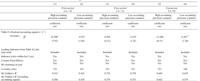
We first present the results without the precision dichotomy. Recall we have no conjectures for the accounting signals over the entire sample. The results, in
19 Berg and Pattillo (1999) assess the pros and cons of the two approaches, and conclude in their Section 3.2 that probits
slightly outperform the signal threshold approach.
20 Gorton (1988), Kaminsky, Lizondo, and Reinhart (1998), Berg and Pattillo (1999), Kaminsky and Reinhart (1999), and
26
Table 5, show that accounting signals overall have no predictive power. Some of the significant one-year ahead early warning indicators are: real exchange rates, industry production, excess real M1 balances, domestic credit, commercial bank deposits, and oil prices, all with the predicted signs. There is certainly much variation in prior studies’ findings on the early warning indicators, but we believe that our findings square well with the last but one column of Edison (2003, Table 5), which shows that these signals have some of the highest probability of predicting a crises when they are emitted. Likewise, Frankel and Rose (1996, p.351) also show that a drop in industry production and a high growth in domestic credit, among other factors, are significant predictors in crashes. These results give us some comfort on the empirical validity of our setting.21 Finally, the lagged dependent variable is not significant in the one-year ahead predictive model, but is in the two-year ahead predictive model. Thus, although crises are not highly autocorrelated events, it is important to control for their dynamics.
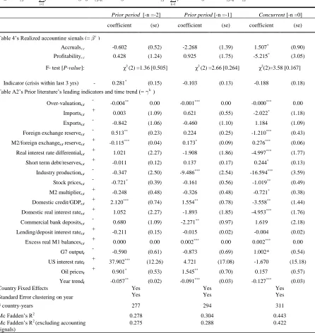
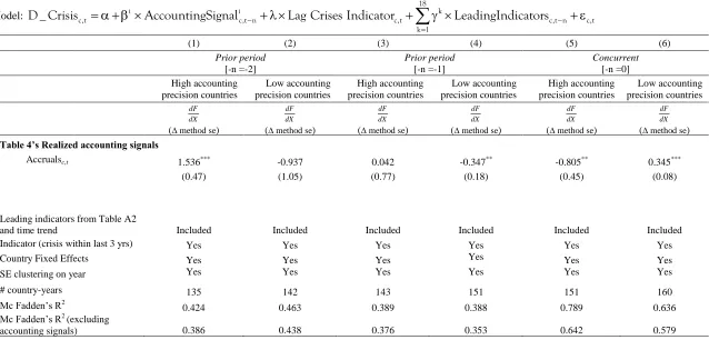
C. Main Results
We now compare the predictive power of the accounting signals across the two groups of accounting precision. Table 6 presents the results. Recall that accruals are adjustments made to the cash flows to compute economic or accounting profits. Holding accounting profits constant, a decrease in accruals implies that a smaller portion of the current economic profit will be realized as future cash flows. In other words, future cash flows are likely to be lower than suggested by current cash flows. A classic example of a negative accrual is a write off. Write-offs immediately recognize the loss of future benefits of some asset. However, this information cannot be gleaned from this period’s cash flows. Another negative accrual is an increase in account payables (e.g., delaying
27
payments to employees and vendors). This accrual recognizes an increase in future cash obligations, an event that has no immediate impact on current cash flows. Thus, decreases in accruals reflect the manager’s recognition of increases
in future obligations (or decreases in future benefits) that are yet to happen, and therefore not evident in current cash flows. A similar argument in the opposite direction can be made for positive accruals (such as an increase in current receivables that will turn into cash later).22
The economic time-series interpretation of accruals above is consistent with the statistical within-firm variation interpretation of the coefficients in the panel regressions in Table 6 with fixed effects. Table 6, Panel A shows that two years prior to the crisis in high precision countries, the accrual coefficient of 20.245 is positive and statistically significant: managers are actually expecting a higher portion of the current economic profits to be realized in the future (i.e., future cash flows are likely to higher than suggested by just the current cash flows). This is consistent with our model which, because of multiplicity considerations, makes no directional predictions on the link between fundamentals and crises for high precision countries: in these countries, the model indicates that self-fulfilling beliefs are more active and crises can hit for a wider range of fundamentals.23
In the year prior to the crisis, accounting signals in high precision countries show no impact, a finding also consistent with the presence of multiplicity in this region. But in the low precision countries, accruals decline significantly at the 5 percent level. This is what our model predicts when it states that low signal realizations are the unique cause of crises in low precision settings.
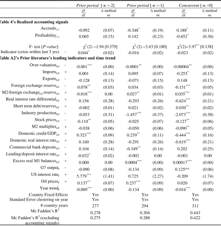
The coefficients of the probit regression cannot be interpreted directly. In Table A3, Panel B, we compute the marginal effect averaged over all the
22 It is for these reasons that Barth, Cram, and Nelson (2001) find accounting earnings and accruals to be superior
predictors of future cash flows than current cash flows themselves.
23 These results are also consistent with Frankel and Rose (1996), Kaminsky and Reinhart (1999), and Rancier, Tornell,
28
observations. In the pre-crisis year for the low precision countries, the coefficient on accruals is -0.346, suggesting that for a .01 decrease in accruals, the probability of a crisis in these countries in the subsequent year increases by 0.346 percent. This is about the same magnitude that Frankel and Rose (1996, p. 362) report for their FDI inflows regressor. A 0.01 decrease in accruals is quite feasible is our sample; Table 4, Panel B indicates that the standard deviation of accruals is 0.268. These magnitudes provide economic plausibility to the important result that pre-crisis accruals are significantly lower only in the low precision countries.24
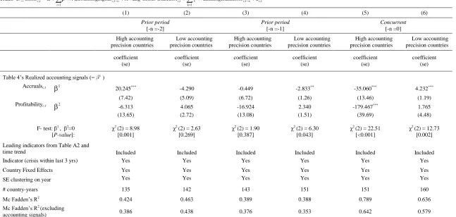
The results on accruals thus far obtain after controlling for profitability. As an additional check, Table 6, Panel B shows that the same results on pre-crisis accruals obtain even after dropping the profitability regressor (the average marginal effects in Table A3, Panel C are also similar). The robustness of the accruals result is particularly valuable because it shows that accounting practices matter: it is the application of accounting rules to the measurement of firm operations that generates critical asset-pricing information. Accounting adjustments thus play the role they are supposed to play (Summers 2000, p.10).25
To investigate our pre-crisis accruals results further, we test if any systematic component of accruals is causing the results. We decompose accruals into
24 Table A3 also reports the standard error of the marginal effects, which are computed using the delta method that
linearizes the average marginal effect using the first order Taylor expansion. The significance of other coefficients in Table A3, Panel B largely line up with Table 6, Panel A. One difference is that the profits in low precision countries in the pre-crisis year are positively significant. Holding accruals constant, an increase in profits suggests an increase in cash flows. One explanation for the positive coefficient on the pre-crisis profits and negative coefficient on the pre-crisis accruals in the low precision countries is that the pre-crisis cash flows are booming, but managers are indicating via accruals that these cash flows are not going to persist in the future.
25 Although the accounting data are impacted by a country’s institutions, the accounting signals could gain power in low
29
changes in current operating asset (ΔCA), changes in current operating liability (ΔCL), and depreciation. At this detailed level of granularity, different firms
could be adjusting different factors of account; so one may not expect any one component of accruals to be the systematic predictor of crises, even when total accruals are. And in fact, we are unable to see any meaningful systematic variation in any particular subset of accruals.26
The crisis year is equally interesting. First, all McFadden R2 are much higher, suggesting that all measures are better at reflecting the occurrence of a crisis than predicting it. The high precision countries consistently show a significant decline in profits and accruals at the end of the crisis year, suggesting that although the causes of the crises were not associated with low signal realizations, the occurrence of crisis is followed by low signal realizations. This aftermath is consistent with the message of Reinhart and Rogoff (2009). However, the same cannot be said of the low precision countries. Although the signals were low in these countries pre-crisis, they show no significant deterioration in the aftermath. The profit effect is neutral and accruals actually pick up significantly after the crisis, suggesting more confidence in the future.
One potential explanation for the above result comes from the cross-sectional variation in the aftermath of crises, as shown in Figures 1-4 of Reinhart and Rogoff (2009). Those figures indicate that many of our low-precision countries show a shorter duration of the aftermath than many of the high-precision countries.27 Reinhart and Rogoff (2009, p.469) themselves make the observation that emerging markets do better than advanced countries in employment recovery, speculating as causes structural macroeconomic factors such as a greater downward flexibility in wages in emerging countries. Such positive economic
26 A similar point is made in a different context by Bertrand, Mehta, and Mullainathan (2002), who argue that because
activities such as expropriation can take many forms, their systematic evidence should be present in overall measures of firm performance measures rather than their specific components.
27 For example, in their Figure 3, the duration of unemployment was about 3 years for the 1997 Malaysian crisis, and about
30
factors could, in the aftermath, increase the coefficient on accruals in the low precision countries. Additionally, the same structural macroeconomic flexibility could have also enabled the companies to cut costs fast enough to the keep the profit effect neutral in the crisis aftermath. Although it is beyond the scope of this study to fully explore the variations in the aftermath (which depend on factors ranging from the impact on imports and exports and the level of foreign currency-denominated debt to post-crisis fiscal and trilemma-related policies), such connections with prior studies, while undoubtedly speculative, serve to further support our model and empirical findings.
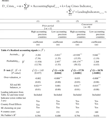
Finally, to complete our model, we include equity prices as an additional regressor. We define stock price movements as the percentage change in the country’s equity index over the year. Table 7 presents the results. The negative predictive significance of the accounting accruals in the year prior to the crisis in low precision countries is robust to the inclusion of the stock price. The stock prices are not a predictor of crises.28 But they fall significantly in the aftermath in both high and low precision countries, suggesting that the low precision countries do suffer a loss of investors, even though their immediate post-crisis profits themselves do not show any significant movement (after controlling for accruals). Our speculative conjecture is that investors appear to be unconvinced about these markets’ future prospects, despite their firms’ efforts to contain the losses.
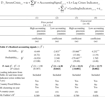
D. Robustness Tests
We next conduct the following additional robustness tests:
(i) Our data do not account for crises that were deterred or did not happen even though they were theoretically likely. To partially account for this omission, we nominate the less severe crises as those falling into these
28 Our estimation technique does not construct the composite signal z’, but instead includes z and p separately. Table 7
31
categories. We repeat our analysis by redefining the crisis year indictor as 1 only if the year after the crisis saw an output loss for that country that was greater than the concurrent sample median (all the other crises thus become non-crises). We obtain similar results in Table A4. Accounting accruals in year -1 are significant negative predictors only in low precision countries. The aftermath results are similar to Table 6, Panel A.
(ii)The descriptive statistics for all the leading indicators are reported in Table A3, Panel B. Some leading indicators have extreme values. The extreme values for the currency overvaluation variable are from Indonesia and Mexico during periods of high inflation. The extreme values for the excess real M1 balances are due to the EU countries that experienced a discontinuity in the M2 measures in 1999. Our main results hold if we winsorize these indicators (Table A5).
(iii) We use an alternative measure of accounting precision based on a user perception of accounting information, as opposed to the properties of reported earnings. We construct an accounting precision measure based on the forecast frequency of financial analysts, who are key users of accounting information. Financial analysts collect, process, and most importantly, disseminate information about a firm to the public. As a result, prior literature argues that the number of analysts following a firm is indicative of the quality of the public information available about the firm (e.g., Lang and Lundholm 1996; Hong, Lim, and Stein 2000). We divide the sample into high and low precision countries using analyst following as the measure, and examine the predictive power of the realized accounting signals.
Table A6 lists the countries’ new partition, which shows a
32
the realized accounting accruals in the year prior to the crisis are a significantly lower only in countries with low analyst following (though the statistical significance is at the 10 percent level). Accruals in year -1 are insignificant in countries with high analyst following. The aftermath looks similar to Table 6, Panel A, though the joint and individual significances are somewhat different. This result suggests that our main findings mostly hold with user perception measures of accounting precision. In addition, this analysis also demonstrates both the importance and the empirical difficulties of identifying the multiplicity threshold correctly.
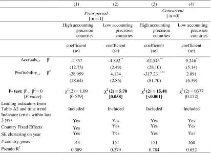
(iv)Finally, Table A7 shows that our main results are robust to switching from a probit to a logit regression model. Accounting accruals in the year prior to the crisis are significant negative predictors only in the low precision countries. The aftermath is similar to Table 6, Panel A as well. Thus, our results are not driven by the functional form of the binary choice model.
IV. Conclusion
Disagreements about basic macroeconomics paradigms (e.g., Solow 2010) suggest that macroeconomics is unlikely to converge on a unifiedtheory of crisis: the underlying phenomena are too complex to be definitively abstracted. Our more modest goal is therefore to empirically show that the global-game coordination models are a viable abstraction of the true complex processes that precipitate crises, after controlling for previously posited determinants.
33
fundamentals are significantly lower only in low precision countries is consistent with our model.
Our findings have two implications. First, as suggested by Summers (2000, p.10) and Rajan and Zingales (1998, p. 569), the application of accounting rules and principles to measure firm operations indeed appears to generate asset-pricing information relevant to macroeconomic phenomena (in our case crises). Second, as financial markets continue to gain prominence in macroeconomic research, global games offer an important insight: improvements in the public signals in such markets do not necessarily offer a monotone improvement in these markets’ ability to allocate resources; investors can also get more unnecessarily “spooked.”
However, such non-convexities do not easily lend themselves to straightforward empirical analyses. It is our position that, in this "age of accounts" (to use Samuelson's (1970, Ch.5) felicitous phrase), innovative use of institutional data such as accounting has the power to overcome these empirical barriers.
REFERENCES
Allen, F., D. Gale. 2000. Financial Contagion. Journal of Political Economy 109:1-33. Andrade, G., S. Kaplan. 1998. How Costly Is Financial (Not Economic) Distress?
Evidence from Highly Leveraged Transactions that Became Distressed. Journal of Finance 53: 1443-1993.
Angeletos, G-M., C. Hellwig, and A. Pavan. 2006. Signaling in a Global Game: Coordination and Policy Traps. Journal of Political Economy 114: 452-484. Angeletos, G-M., C. Hellwig, and A. Pavan. 2007. Dynamic Global Games of Regime
Change: Learning, Multiplicity and Timing of Attacks. Econometrica 75: 711-756.
Angeletos, G-M., I. Werning. 2006. Crises and Prices: Information Aggregation, Multiplicity, and Volatility. American Economic Review 96: 1720-1736.
Atkeson, A. 2000. Discussion of Morris and Shin’s “Rethinking Multiple Equilibria in Macroeconomic Modeling.” NBER Macroeconomics Annual 15. Cambridge, MA, MIT Press.
Ball, R., S. Kothari, and A. Robin. 2000. The Effect of International Institutional Factors on Properties of Accounting Earnings. Journal of Accounting and Economics 29: 1-51.