City, University of London Institutional Repository
Citation:
Neuberger, A. (2012). Realized Skewness. The Review of Financial Studies, 25(11), pp. 3423-3455. doi: 10.1093/rfs/hhs101This is the accepted version of the paper.
This version of the publication may differ from the final published
version.
Permanent repository link:
http://openaccess.city.ac.uk/15210/Link to published version:
http://dx.doi.org/10.1093/rfs/hhs101Copyright and reuse: City Research Online aims to make research
outputs of City, University of London available to a wider audience.
Copyright and Moral Rights remain with the author(s) and/or copyright
holders. URLs from City Research Online may be freely distributed and
linked to.
City Research Online: http://openaccess.city.ac.uk/ [email protected]
REALIZED SKEWNESS
Anthony Neuberger
Warwick Business School Warwick University
Coventry CV4 7AL United Kingdom (44) 24 7652 2995
The third moment of returns is important for asset pricing. But the third moment, particularly of long horizon returns, is hard to measure precisely. This paper proposes a definition of the realized third moment that is computed from high frequency returns and from option returns. It provides an unbiased estimate of the true third moment of long horizon returns. The novel methodology is used to demonstrate that the skewness of equity index returns, far from diminishing with horizon, actually increases with horizons up to a year, and its magnitude is economically important.
While standard approaches to asset pricing concentrate largely on the first and second moment of returns, there is mounting evidence that higher moments are also important. The literature going back to Kraus and Litzenberger (1976), and including more recently Harvey and Siddique (2000), Ang, Hodrick, Xing and Zhang (2006), Ang, Cheng and Xing (2006) and Xing, Zhang and Zhao (2010), suggests that the asymmetry of the returns distribution both for individual stocks and for the market as a whole is important for asset pricing and investment management. Skewness is central to the debate on the role of large rare disasters in explaining the equity risk premium (Rietz (1988), Longstaff and Piazzesi (2004), Barro (2009), and Backus, Chernov and Martin (2011)). Carr and Wu (2007) document the time varying implied skew in foreign exchange markets, and Brunnermeier, Nagel and Pedersen (2008) relate the forward premium puzzle to the skewed distribution of currency returns.
has side-stepped the problem by focusing on skewness and co-skewness at monthly or higher frequencies. But skewness, unlike variance, does not scale nicely with horizon, and it is not clear what the relationship is between skewness at short and long horizons, or why asset prices in an economy with well-capitalized long term investors should be heavily influenced by the characteristics of short horizon returns.
Skewness in long horizon returns comes from two sources: the skewness of short horizon returns and the correlation between returns and volatility innovations (the leverage effect). In this paper, I show how to use high frequency1returns to compute the third moment of long horizon returns. The computation uses option return data as well as returns on the underlying asset. The option returns help capture the leverage effect. The existence of strong negative correlation in the equity market has been much discussed since being documented by Black (1976) and Christie (1982), and turns out to be much more important than the skew in high frequency returns in delivering skew in index returns at long horizons.
Because of the close analogy with the use of high frequency returns to compute realized variance, I call the computed quantity the realized third moment. The realized third moment is an unbiased estimate of the true third moment. The lack of bias is not based on any model; it only requires that prices are martingale. It is robust to price jumps and discrete sampling. I show that this property of freedom from bias is sufficient to define the realized third moment uniquely. The realized third moment can then be normalized by dividing by the variance to the power of 3/2, to give the realized skewness coefficient.
As a by-product of the derivation of the realized third moment, a new definition of realized variance is also proposed; unlike the standard definition, it provides an unbiased estimate of true variance, even in the presence of jumps. The parallel with variance goes further. Just as there is a model-free strategy to replicate a variance swap, a swap where the floating leg is the realized variance, so there is a model-free strategy to replicate a skew swap, one where the floating leg is the normalized realized third moment. Carr and Wu (2009) use variance swaps to explore variance risk premia; Kozhan, Neuberger and Schneider (2011) use skew swaps to explore the existence and behavior of risk premia associated with skew.
I show, using daily data, that the skew in the equity index market, far from declining with horizon as would occur under an iid process, is actually higher at one year than it is at one month. Furthermore the increased precision of measurement makes it possible to document that the skew in index returns is time varying, and that the degree of variation is economically significant.
These findings are relevant to the debate on the role of large disasters in explaining the equity premium. In reviewing the evidence, Backus, Chernov and Martin (2011, p1970, “BCM”) note that “in virtually all of this research [starting with Rietz (1988), followed by Longstaff and Piazzesi (2004), Barro (2009) and others], the distribution [of log returns] is modeled by combining a normal component with a jump component. The jump component, in this context, is simply a mathematical device that produces nonnormal distributions”.
(see BCM, Table 3), in contrast with a figure of around -1 suggested by the analysis presented here. If the horizon of the representative agent is of the order of years rather than days, the calibration of the model to daily returns may understate the role that rare disasters play in asset pricing. High frequency models used to investigate large disasters need to capture the dependency between returns and variance over long horizons that is observed in the data.
Previous work on trading the skew includes Schoutens (2005) and Schoutens, Simons, and Tistaert (2005) who describe swap contracts that pay the sum of cubed daily returns. The swaps capture the third moment of high frequency returns, but do not take account of the leverage effect that heavily affects the third moment of returns over the life of the swap. Bakshi, Kapadia and Madan (“BKM”, 2003) show how the implied moments and skewness coefficient of the risk-neutral probability density can be recovered from option prices. The implied density in general differs substantially from the density under the physical measure (see Carr and Wu, 2009). There is no obvious way of relating the implied BKM skew at any horizon to the actual behavior of high frequency returns up to that horizon.
1.
Skewness of Equity Index Returns
Daily returns on the S&P500 are on average negatively skewed. The skewness coefficient of excess log returns2 over the period July 1963 to June 2011 is -0.83. The result appears to be significant; thep-value against the null that the skew is positive is 4.3%.
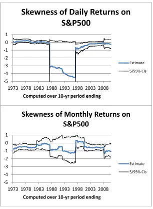
But even with a very long run of data, the precision of the estimate is low, and the point estimate is heavily influenced by outliers. Specifically, the conclusion that daily returns are negatively skewed relies heavily on one observation – 19 October 1987. The top panel of Figure 1 shows the skewness coefficient and the 5/95% confidence intervals computed from rolling ten-year windows. The impact of the 1987 Crash is obvious. For most of the windows (including periods affected by the Crash) the hypothesis that the skew is positive cannot be rejected at conventional significance levels. The weakness of the evidence for negative skewness of daily returns has been noted by other authors including Kim and White (2004).
When the same technology is applied to monthly returns over the same period, the conclusions are somewhat different. The point estimate for the period as a whole is -0.74; the
p-value is 0.1% suggesting strong evidence for negative skewness. The lower panel of Figure 1 shows the rolling ten-year estimates for monthly returns. The 1987 Crash does not stand out. While the point estimates from the rolling estimates are generally negative, the data only rejects the null of zero or positive skewness in the early and later parts of the period; in most of the middle period, the null cannot be rejected.
the skewness coefficient would be proportional to 1 n. There is no evidence of such a decline in skewness with horizon in the data. To explore the relation between skewness coefficients of daily and monthly returns more fully, I bootstrap the daily returns to generate a synthetic time series, and compute the population skewness of both daily and monthly returns. The results are plotted in the top panel of Figure 2. The lower panel does the same thing using monthly and annual rather than daily and monthly returns.
The hypothesis that returns are iid and the skew at the monthly horizon derives from the skew at the daily horizon is firmly rejected by the data (p-value of 0.02%), and the hypothesis that annual skew is generated by monthly skew is also rejected (p-value of 4.76%). This is clear evidence that the distribution of low frequency returns is heavily influenced by serial dependence in high frequency returns. If high frequency returns are to be used to improve the estimate of the skewness of low frequency returns, it must be done in a way that reflects the serial dependencies that are manifest in the data.
2.
Arithmetic Contracts
This section introduces the Aggregation Property – the property that ensures that the quantity measured using high frequency returns is an unbiased estimate of its low frequency counterpart. The goal is to get a good measure of the third moment of returns, and that will be achieved in section 3. This section looks at price changes rather than returns because the mathematics are simpler, and the underlying logic more transparent.
St
t
0,T
is a positive adapted variable defined on a standard filtered probabilityspace
,F, F
t t 0,T ,
. t
. denotes .Ft. The distribution ofSTis assumed such thatexpectations of ST and functions of ST such as ST2, ln(ST) and ST ln(ST) exist.
0 0 1 ...
t t tN T
T is a partition of [0,T]. max
i i1
i t t
T is the mesh of T. For a
process x, xi is shorthand for .
i t
x xidenotes xixi1. For a function g(.),
g
xT
is
shorthand for
1
N
i i
g x
I will sometimes refer to the period [0,T] as a month, and the length of the sub-period as a day, but obviously nothing hangs on this. In the present section, references to variance and skewness relate to the distribution of price changes and not of returns. To avoid irrelevant complications with interest rates and dividends, I work throughout with forward prices, so all trades, whenever entered into, are for settlement at timeT.
2.2 The Aggregation Property
For any martingaleS
2
2
0 0 .
S
ST T
(1)
There are several interpretations of this equation. The left hand side is
2 0 ST S0 .measure, this is the true variance of S.Equation (1) then says that if prices are martingales, the sum of squared daily price changes (therealized variance) is an unbiased estimator of the true variance. If the measure is a pricing measure, it says that the fair price of a one-month variance swap computed daily (a swap that pays the realized daily variance over a month) is the same as the price of a contingent claim that pays
ST S0
2. Indeed, since the relationshipholds under any pricing measure (since the process is martingale under any pricing measure), it also implies that a variance swap can be perfectly replicated if the contingent claim exists (or can be synthesized from other contingent claims), and the underlying asset is traded. It is reasonable to call the time 0 price of the claim theimplied variance.
The relation between the true variance of the monthly price change, the realized variance of daily changes over the month and the implied variance of one-month options at the beginning of the month holds exactly, whatever the price process and whatever the length and number of sub-periods, provided only that S is a martingale. It depends on the interchangeability of the summation and the square function under the expectations operator.
In order to generalize the notion of true, realized and implied characteristics, some more definitions are needed. If g is a real-valued function and X is an adapted (scalar or vector) process, then (g;X) has theAggregation Propertyif, for any times 0 s t u T,
.sg XuXs sg Xu Xt sg XtXs
(2)
Applying the Law of Iterated Expectations, if (g;X) has the Aggregation Property then
0 0 0
g XT X
g X T
for any partition T.
g
XT
characteristic; and 0g X
T X0
is the implied characteristic if the measure is a pricingmeasure, or thetruecharacteristic if the measure is the physical measure.
(g;S) has the Aggregation Property for any martingaleSwheng(x) =x2. Proposition 1 below shows that no other interesting functions have the Aggregation Property. But there is no reason to require that X = S. Let X(S) be a vector-valued process
S V St, t
T :t
0,T
where V St
T Var St
T , the variance of ST conditional on information at t. G is the set ofanalytic functionsgsuch that
g X S;
has the Aggregation Property for all martingalesS.Proposition 1: Gconsists of the functions
2
3
0 1 2 3
, 3 .
g S V h V h S h S h S S V (3)
where the {hi} are arbitrary constants.
Proof:see Appendix 1.
G is spanned by four functions: g0 V andg1S, which are uninteresting,
22
g
S
, which is the variance and is familiar, andg
3
S
3
3
S V
.
The truecharacteristic ofg3is
0 3 0 0 0 3 0 0
3
0 0 0 0
3
0 0
, , (since 0)
3 (definition of )
(since is a martingale).
T T T T
T T
T
g S S V V g S S V V
S S V S S g
S S S
Hence, the characteristic captured by g3 is the third moment. The left hand side of
equation (4) is the true third moment of the price change over the month. The realized third
moment is
g3
S, V
S 33 S V
T T
. The Aggregation Property means that the
realized third moment equals the true third moment in expectation
3
30 3 0 0 .
S S V ST ST
(5)
Equation (5) is significant in several respects. It shows that skewness in low frequency returns derives only in part from the skewness in high frequency returns. The second source (and indeed the only source when S is a continuously sampled continuous martingale) is the covariation between shocks to the price level and shocks to future variance.
It also shows how high frequency data can be used to provide more efficient estimates of the skewness in price changes over a period. This improvement rests on two assumptions: the discounted price process is a martingale, and the variance of the terminal price is in the observer’s information set. Third, if a pricing measure is used, the right hand side is the implied third moment (which can be inferred from the prices of options that mature at timeT). The difference between the implied and realized third moments can be used to detect and analyze risk premia associated with skewness.
square contract, a security that pays ST2. Under the pricing measure, the price of the contract on dayiis
2 2 2 2
2
since .
i i T i i T i
i i i i T
P S S S S
S V S S
(6)
The gain from holding one square contract for one period is
21 1 2 1 1.
Pi Si S Si i Vi (7)
Suppose an agent enters into a one month third moment swap on day 0, paying floating and receiving fixed, with the realized third moment being computed from daily prices. She uses the fixed payment to buy a contract that pays the cube of the price change
over the month. She hedges by holding -3(Si-S0) square contracts and
2 0
3 SiS Vi forward contracts over dayi. If her initial wealthW0= 0, her terminal wealth is
3 3 0 1 1 2 20 1 1 1 0 1
0 0
3
3 2 3 .
T T
N N
i i i i i i i i
i i
W S S S S V
S S S S S V S S V S
T (8)3.
Geometric Contracts
3.1 Generalized Variance
Financial economists are interested in the behavior of returns, not price changes. It is tempting to apply the theory in the previous section directly to the log price,
s
t
ln .
S
t But the log price is not a martingale either under a pricing measure or, in general, under the physical measure. In looking for a definition of implied and realized variance of returns, I start from the premise that it is important to keep the Aggregation Property. The price for this is a relaxation of the definition of variance.Let f be an analytic function on the real line with the property that
20
lim 1
x f x x .
Given a process s, define the process vtf
sT tf s
T st
. I will call vtf
sT ageneralized varianceprocess fors.3
The variance measures that are widely used by academics and practitioners (squared net returns and squared log returns) conform to the definition of generalized variance. Two other generalized variance measures,vLandvE, turn out to be important
where 2 1 ,
where 2 1 .
L x
t t T t
E x x
t t T t
v L s s L x e x
v E s s E x xe e
(9)
2 1 ln so ln ln 2;
2 ln 1 so ln ln 2.
L T T L
t t t T t t
t t
E T T T E
t t t T T t t t t
t t t
S S
v S S v
S S
S S S
v S S S S S v
S S S
(10)
In a Black-Scholes world, where the underlying asset has constant volatility , the price of a log contract, one that pays lnST, is lnSt 2
Tt
2, soL t
v is the implied
Black-Scholes variance of the log contract. It is the same as the model-free implied variance (MFIV) of Britten-Jones and Neuberger (2000). Similarly,vtEis the implied Black-Scholes variance of the contract that paysSTlnST. I call it entropy because of the functional similarity to entropy as
used in thermodynamics and information theory.
The following properties of the log and entropy variance will be useful. From the first line of (10)
1 1
2 2 so
2 0. L
t t t T
L
t t t
v s s
v s
(11)
Similarly, from the second line
1 1 1 1 1 1 2 2so 2 2 2 0
which implies that 2 0.
t T t t t
s E s
t t t T
s s E E E
t t t t t t t
s E
t t t
e v s s e
e e v v s s v s
e v s
3.2 Aggregation with Returns
Let G* be the set of analytic functions g where
g X S;
has the AggregationProperty for any positive martingale S, where X(S) is the vector process (s,v) with slnS
andvis a generalized variance process fors.
Proposition 2:the setG*comprises the following functions
2
1 2 3 4 5
4 5
5 4
4 5
, 1 2 2
where are arbitrary constants, with the following constraints:
if 0, and 0;
if 0, and 0;
if 0, is any generalized varianc
s s
i
L E
g s v h s h e h v h v s h v s e
h
h v v h
h v v h
h h v
e measure.
(13)
Proof:see Appendix 1.
I now examine the properties of three particular members ofG*.
Proposition 3: the function gM
s es1 is a measure of expected return and has theAggregation Property.
Proof:The Aggregation Property follows immediately from Proposition 2 withh2= 1, and h1
=h3=h4=h5= 0. The implied characteristic is 0
ST S01
and is the mean return.■3.3 Variance of Returns
Proposition 4: the function gV
s 2
es 1 s
is a measure of variance and has the Aggregation Property.Proof:The Aggregation Property follows from Proposition 2 withh1= -2,h2= +2, h3 =h4=
h5= 0. gV
x x2O x
3 , sogVis a generalized variance measure. ■With this unconventional definition of variance, the implied variance at timet,IVt, is
the price of a contract that pays gV(sT-s0), so IVt vtL. The realized variance is
2
1
V
s t
RV g s e s
T T
. Thetrue varianceis TVt t2
ST S0 1 ln
ST S0
where the expectation is under the physical measure, rather than under a risk-adjusted measure. The true variance is unobservable; the realized variance is an unbiased estimate of the true variance if the price process is martingale; the implied variance is an unbiased estimate of the true variance in the absence of a variance risk premium.The definition of implied variance is the same as the standard MFIV. The realized
variance differs from the conventional definition,
s 2, Tbut is found in Bondarenko
the Aggregation Property means that replication is perfect for every price path and every partition, and is robust to jumps.
In practice, with reasonably frequent rebalancing, the two measures of realized variance are very similar. This is not surprising since they are both generalized measures of variance. The monthly realized volatility of the S&P500 computed using daily returns has averaged just over 18% (annualized) over the last ten years (2001-2010). The root mean square difference between the two measures over that period is 0.06%. Since the 1950s the biggest difference between the two measures was in the month of October 1987 when the conventional measure of realized volatility was 101.2%, while the alternative measure registered 98.8%.
There do not appear to be any strong theoretical arguments for preferring the conventional definition of realized variance (apart from the fact that it is well established both in the academic and practitioner communities). The main justification given in the literature for the conventional measure of realized variance is that it converges to the quadratic variation as the mesh size becomes small. The quadratic variation is important because it is an unbiased estimate of the conditional variance of the log price process under certain conditions (see Andersen, Bollerslev, Diebold and Labys, 2003, Theorem 1 and Corollary 1).4But, as the following Proposition states,RVtoo has this property when the process is a diffusion.
Proposition 5:if f is an analytic function on the real line such that
20
lim 1
x f x x , then for
any continuous semimartingale s, the associated realized variance
f
sT
converges in
Proof:see Appendix 1.5
In the empirical sections of this paper, I use the term variance in the sense of Proposition 4.
3.4 The Third Moment of Returns
Proposition 2 also shows how to construct a definition of the realized third moment of returns, one that closely resembles the definition already established for price changes.
Proposition 6: gQ
s, vE
3vE
es 1
K
s , where K
s
6 ses2ess2 ,approximates the third moment of log returns and has the Aggregation Property.
Proof:gQhas the Aggregation Property by Proposition 2 withh1= 6,h2= -12,h3= -3,h4= 0,
and h5 = 3. gQ
sT s vt, tE vTE
3vtE
ST St 1
K s
T st
. With the price following a martingale, the first term is zero in expectation.
3
4K x x O x and converges to the third
moment of returns whenxis small. ■
The implied third moment,ITMt, is the price of a claim that pays gQ
sT st,vtE
. It can be replicated exactly from forward contracts, entropy contracts and log contracts. The price of the claim is
3 .
E L
t t t
In a Black-Scholes world, all options trade on the same implied volatility, the log and entropy variances are equal and ITMt = 0. As Bakshi and Madan (2000) show, any general
claim can be replicated by a portfolio of vanilla options; the replicating portfolio for the third moment claim is
0
2 0 2
6 ( ) ( ) 3 ,
t t S E t t S t tk S S k
k dk k dk v
S k C S k P F (15)
where C(k) andP(k) denote a call and a put with maturity T and strikek, and Fis an at-the-money forward contract with the same maturity.
The implied third moment is thus the price of a portfolio that is long out of the money calls and short out of the money puts. By dividing the implied third moment by the implied variance to the power of 3/2, the implied skewness coefficient (ISC) can be computed
3 2 3 2
3 = = . E L t t t t L t t v v ITM ISC IV v (16)
The realized third moment is RTMt
gQ
s, vE
T
; it is natural then to define the
realized skewness coefficient
3 2 3 2
3 1 = . 2 1
E s t t s tv e K s
Finally, the true third moment and true skew coefficient can be defined as
,
Q E
t t T t t
TTM g s s v and TSCt TTM TVt
t 3 2.The realized third moment is an unbiased estimator of the true third moment if prices of the underlying asset and of the entropy contract defined on it are martingales. The realized skew coefficient is not necessarily an unbiased estimate of the true skew coefficient since the ratio of two unbiased estimators is not in general an unbiased estimate of the ratio.
A third moment swap, where the floating leg is the realized third moment and the fixed leg is the implied third moment, can be replicated perfectly by dynamic hedging, trading the entropy contract and the forward contract. To replicate the swap, it is necessary that an entropy contract with maturity Tis traded (or equivalently, that calls or puts with maturityT
and all possible strikes are traded, so that the entropy contract can be replicated). An agent who writes the swap, receiving fixed and paying floating, receives net
0 0
3 vE vL
3vE es 1 K s . T(18)
To hedge her position she needs to buy six log contracts, with terminal pay-off 6lnST.
This costs 6lnS03v0L (by (10)). She also needs to hedge dynamically by holding a long
position of 6 Sientropy contracts on day i (contracts that have a pay-off of ST lnST) and a
3.5 True and Realized Third Moments when Prices are not Martingales
The realized third moment is useful for estimating the true third moment of returns. Proposition 6 shows that the realized third moment is an unbiased estimator of the true third moment when prices are martingale. But when prices are not martingale, it is a biased estimator. The following proposition characterizes the bias under the much weaker assumption that the process is ergodic.
Proposition 7 The difference between the true and realized third moments depends on the
cross-correlation between returns on the underlying asset and the returns on a hedged option
position. Specifically
1 10 1 1 1
1 0 0
1 2
6
where is the price of the entropy contract at time , and 1 ln . T T
u u t u t t t
u t u t t
E t
t t t t
t
E S S S E S
TTM RTM
S S S S
E
E t S v
S
(19)If changes in the term structure of volatility are parallel, and the correlation between
returns on the underlying asset on day t and returns on a fixed maturity delta-hedged entropy
contract on day t+n isry(n)then
,
1
where , .
0 1 T TM ry n T TM ry
w n T n
T n T n TTM
w n T
RTM T T
(20)The difference between the true variance of a price series and its realized variance
,
where
,
,
T V rr v n T
T n TV
w n T n w n T
RV T
(21)
Proof:in Appendix1.
The first part of the proposition says that if the expected return on an asset is positively (negatively) correlated with its variance risk premium in prior or in subsequent periods, then the realized third moment is a downward (upward) biased estimate of the true third moment. Under the hypothesis that the underlying asset and the entropy contract are martingales, the expected return on the asset and its variance risk premium are zero, and hence there is no bias.
The second part expresses the bias in terms of the cross-correlation between the expected return and the variance premium. The assumption that shifts in term structure are parallel allows the return on an option contract with a maturity that declines in time to be replaced by the return on a duration matched constant maturity option.
The third part, concerning the relation between realized and true variance is well-known in the literature (see Campbell, Lo and MacKinlay (1996) page 49). The relationship between realized variance estimates computed using different horizons has long been used as a test for serial correlation in returns (Lo and MacKinlay, 1988).
4.
Simulations
offers more precise estimates. In the presence of equity and variance risk premia, Proposition 7 shows that the estimates are biased. In this section, simulation is used to quantify both the improvement in precision and the bias.
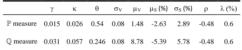
The process that is simulated is the SVCJ stochastic volatility model of Duffie, Pan and Singleton (2000) with contemporaneous jumps in the underlying and volatility
1
S t Z S t
t t t
t
V V
t t V t t t t
dS
dt V dW e dN
S
dV V dt V dW Z dN
(22)
Sis the price of the underlying,Vis its spot variance,WSandWVare Brownian processes with correlation,N is a Poisson process with intensity,ZSis normally distributed with mean S
and standard deviationS, whileZVis distributed exponentially with meanV. Expressions for
the unconditional true, implied and realized moments of -horizon returns under the SVCJ model can be obtained analytically. They are set out in Appendix 2.
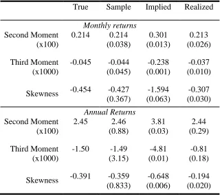
each of 22 days. For each run, the distribution of the 200 monthly returns is used to compute the sample second and third moments as well as the skewness coefficient. The monthly realised and implied moments are calculated and averaged over the 200 months.
The top panel of Table 2 shows that the sample variance of monthly returns computed over 200 months provides a fairly precise and unbiased estimate of the actual variance. The unconditional variance of monthly returns implied by the parameters in Table 1 is 0.214 x 10⁻²; the sample estimate has a standard deviation of 0.038 x 10⁻². The estimate of the third moment also appears to have little bias, but has much greater noise. The standard deviation of the third moment is of similar magnitude to its true value; 200 months is too short a period to reject the hypothesis that monthly returns are positively skewed.
The implied moments have far smaller standard deviations than their sample counterparts; this is to be expected since they are beginning-of-month expectations rather than end-of-month out-turns. They are strongly biased because of the risk premia in option prices, reflected in the large difference between the physical and risk-adjusted parameters in Table 1.
speed of mean reversion () of volatility under the two measures. Mean reversion is twice as large under the risk adjusted measure as under the physical measure. This reduces the beta of implied variance on instantaneous volatility, and so reduces the magnitude of the covariation between implied variance and returns.
BCJ’s estimate of the difference in the speed of mean reversion under the two measures (QP) is driven by the estimated diffusive risk premium (which they call V). As they note (BCJ, 2007, p 1476) it is hard to estimate the sign of the diffusive risk premium let alone its magnitude. While it is clear that this premium may give rise to significant bias, the sign of the bias that arises in practice cannot be identified with confidence.
The implications for the estimates of the skewness coefficient follow immediately from the estimates of the second and third moments. The sample estimate is very noisy, with a standard deviation almost equal to its mean. Although both moment estimates are unbiased, the sample skewness coefficient is biased. The implied skewness coefficient is much more precise, but is more than three times too large, while the realized estimate is also biased being only two thirds of the true value.
The main conclusions that can be drawn from the simulations is that realized skewness provides a far more precise estimate of skewness than does the sample skewness, but it is subject to bias if the risk neutral speed of mean reversion in volatility differs from its physical counterpart. Variance risk premia that do not affect the covariation between returns and implied volatility (such as the variance jump risk premia in the SVCJ model) have no effect on realized skewness though they do give rise to bias in the implied skewness.
5.
Skewness of Equity Index Returns
5.1 The Term Structure of Skewness
The empirical analysis in this section is based on European options written on the S&P500 index traded on the CBOE obtained from OptionMetrics. The one month options mature every month, while the 3, 6 and 12 month options mature every three months. In each of the series, the first period starts in December 1997 and the last starts in September 2009. The data set includes closing bid and ask quotes for each option contract along with the corresponding strike prices, Black-Scholes implied volatilities, the zero-yield curve, and closing spot prices of the underlying. Entries with non-standard settlements are deleted.
Put and call option prices for every strike at each maturity are computed by interpolating implied volatilities between quoted strike prices using a cubic spline. Outside the quoted range, the implied volatilities at the lowest and the highest strike price are used. The Log and Entropy Contracts are synthesized from the continuum of conventional options and
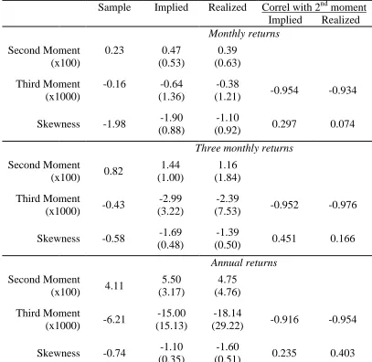
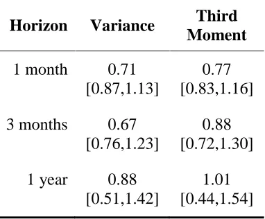
Table 3 shows summary statistics at different maturities. Realized variance is on average lower than implied variance, which is consistent with a positive variance risk premium, and both increase linearly with maturity as one might expect. The realized and implied third moments are negative at all maturities7. They increase with maturity faster than linearly. The implied third moment is on average larger (in absolute size) than the realized third moment at short maturities, but the difference appears to vanish or reverse at longer maturities. The skewness, both implied and realized, exceeds -1 on average at all maturities. Implied skewness appears to decline with maturity, whereas realized skewness on average actually increases with maturity.
Both the second and third moments, whether realized or implied, are highly skewed and variable. They are very highly (negatively) correlated with each other, with correlations in excess of -0.9. The skewness coefficients tend to be much less variable and to be distributed symmetrically. They are much less highly correlated with variance; the sign of the correlation coefficient is positive implying that the higher the variance the less skewed the distribution, but the correlations are all below 0.5.
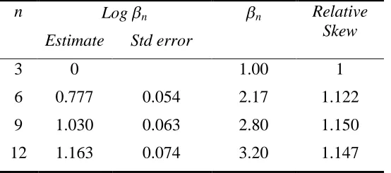
To analyze the term structure of skewness, define Yt,n as the realized third moment
accumulated over the quarter starting at time t using options that mature at time t+n where time is measured in months. The Y are all negative, and are highly correlated in the cross-section, with the magnitude increasing with maturity. Table 4 reports the results of the regression
, ,3
3, 6,9,12log log
t n t i i t n
i
whereDi is a dummy that takes the value of 1 if n = i, and zero otherwise, and is an error
term. The estimated value of6 is 2.17, so the realized skewness over a quarter using options
that expire three months after the end of the quarter is 2.17 times as high as the realized skewness computed using options that expire at the end of the quarter. This implies that the realized third moment over six months is 3.17 its value over 3 months. Realized variance is linear in horizon, so the realized skewness coefficient over six months is 3.17/21.5 = 1.12 times its value over three months. The increase is statistically significant; log3would need to
be below 0.60 for the skewness to be lower at six months than at three, and t(log3-0.60) =
3.21.
The point estimate of relative skewness increases from 1 at three months to 1.12 at six months, and to 1.15 at nine and twelve months, though the increases beyond six months are not statistically significant. The panel regression of Table 4 therefore confirms the impression given by the population averages of Table 3 that realized skewness rises with horizon up to six months, and shows no evidence of decline in horizons up to one year.
This shows that the realized second and third moments both over-estimate the true moments at all maturities, with the effect being more important (and more significant statistically) for the variance than for the third moment, and for shorter horizons than for longer horizons. It is not possible to draw firm conclusions about bias in the skewness coefficient since it is the ratio of two biased estimates, but at the very least one can say that the data do not suggest that the realized skewness over-estimates the true skewness, and they also suggest that any bias in the moment estimates attenuates with maturity.
The analysis of realized skewness of index returns at horizons of up to one year shows that returns are strongly negatively skewed at all horizons (with a skew coefficient in excess of -1), that there is no evidence at all that skewness declines with horizon and some evidence that it actually increases for horizons up to six months.
5.2 Time Variation in Skewness
Realized skewness is quite volatile. Table 3 shows that the realized skewness of the S&P500 on a quarterly horizon has averaged -1.39 with a standard deviation of 0.5. The following forecasting model is used to investigate whether this variation is predictable or whether it is just noise
, 1 , 2 ,
for 1,3, 6 and 12, and min 3, .
t t n t t n t m t t n
RSC ISC RSC
n m n
(24)
HereRSCt,t+n , the realized skew from timettot+n, is forecast usingISCt,t+nthe skew
between 10% and 25% of the variation in the realized skew being predictable using simple explanatory variables. The lagged realized skew enters in with positive sign for shorter maturities suggesting that the skew risk premium is predictable, but the magnitude is small. The coefficient is not statistically significant at longer horizons.
Figure 3 shows the relationship between realized and predicted skew graphically at the quarterly horizon, and demonstrates significant time variation in the skew, with predicted skew varying between -1.0 and -1.8 over the period. Interestingly, the period when index volatility was very low by historic standards (2003-7) was also one of relatively high skewness, while in the volatility spike of 2008 skewness was actually rather low.
5.3 The Economic Significance of Index Skewness
To quantify the economic significance of the skewness of index returns, I compute the Markowitz risk premium (expressed as a rate of return) that a rational agent with constant relative risk aversion would demand to compensate for the risk of investing 100% in the market rather than 100% in the riskless asset over a particular horizon . Let r denote the excess log return on the asset. In the classic case of an asset with constant volatility and zero drift (Merton, 1969), the premium required is 1 2
2 .
When r is not lognormally
distributed, the premium depends also on higher moments (as noted for example by Kraus and Litzenberger, 1976), and the premium rate required is
1
log
. 1
r
e
t r f t r
m t e e (26)
for some functionf. Then
1 . 1 f (27)fis calibrated to meet four conditions: the probability density integrates to 1, the price is martingale, and the distribution matches the log and entropy variances
(0) (1) 0 11 1 1;
1 1;
2 ' 0 2;
2 ' 1 2.
f
r f
f
L L
f
r E E
e
e e
r v f e v
re v f e v
(28)
To evaluate the functionf(t) at t= 1- I extrapolate using a cubic polynomial that fits the four conditions in (28)9. This allows the premium to be expressed as a function of the variance (TV) and the third moment (TTM) of the returnr
1 1 1 2 1 . 2 3L E L
f
v v v
TV TTM (29)
Using the mean observed realized variance and third moment of the S&P500 over 1997-2009 from Table 3 as estimates of the true variance and third moment, this implies that for an investor with = 2, the required risk premiumis 4.83%/year at the monthly horizon; had the distribution been unskewed (with vE = vL) the premium would have been 4.68%, a difference of 15 basis points annually. At longer horizons, the skew risk premium is higher. For example, for an investor with a one year horizon, the required risk premium is 5.35%/year, against 4.75% for a symmetrical distribution – a skew risk premium of 60 basis points annually.
At higher level of risk aversion, the risk premium is also higher, and the skew risk premium is more important both absolutely and relatively. So with = 3, the skew risk premium at one year contributes 181 basis points to a total risk premium of 8.94%.
This analysis suggests that the levels of skewness observable in US stock market returns, particularly at long horizons, and the predictable variability in the levels of skewness documented in this paper are economically as well as statistically significant for investors with quite moderate degrees of risk aversion.
6.
Conclusions
intervals are wide, and the results are insignificant in many ten year sub-periods. There is however strong evidence that the distribution of long horizon returns can only be explained by serial dependencies in the data, and is inconsistent with an iid model of the returns process. There is a need for a methodology to measure the skewness of long horizon returns that is far more precise than simply using the sample skewness, and which respects the serial dependencies.
In the case of the second moment of returns, the problem has been addressed by using high frequency returns to compute the realized variance over long horizons. The key property of realized variance is that it is an unbiased estimate of the true conditional variance. In the paper this property has been formalized as the Aggregation Property. The standard definition of realized variance needs to be slightly modified so that it too has the Aggregation Property. More importantly, there is a unique definition of the realized (and true) third moment under which the realized third moment is an unbiased estimate of the true third moment. Calculating the realized third moment requires data on option price returns as well as the returns on the underlying.
the risk premium required by a rational investor for holding the market. This is particularly marked for investors with long horizons.
There are many further research questions that could usefully be explored with the use of realized skewness. The examination of the relationship between implied variance and realized variance, and the existence of variance risk premia by Carr and Wu (2009) could readily be extended to skewness risk premia both in the equity index market (as in Kozhan, Neuberger and Schneider (2011)) and in other financial markets. The evidence on the pricing of skewness and coskewness presented by Ang, Hodrick, Xing and Zhang (2006) could be refined using a definition of skewness with a more rigourous theoretical basis.
APPENDIX 1 - PROOFS
Proof of Proposition 1
It is straightforward to prove that all members ofGhave the Aggregation Property; all that is needed is to substitute (3) into (2). Proving the converse, that all analytic functions that have the Aggregation Property are inG, is more complicated.
Let be a random variable with
0 and 2
, and g an analytic
function that has the Aggregation Property. Consider two processes with t
0,1, 2
. The firstis given by S0 = S1= 0, S2 = . S is clearly martingale. The process (S, V) is (0,(0,
. For the Aggregation Property to hold
,
0, 0
,
.g g g
(30)
It follows thatg(0, 0) = 0. The second process forSis
Pr
0 , with 0 and 1 0.
Pr 1
u u
ud u d
d d (31)
Sis martingale. The process (S,V) is
0
2 2 2
0
, , 0 Pr
0,
, 0 , 0 Pr 1
where 1 .
u u
V
d d
V u d
(32)
0 0
0 0
, 1 ,
, , 1 , 1 0, 0 .
g u V g d V
g u V g g d V g
(33)
Simplifying, and using the fact thatg(0, 0) = 0, gives
, 0
,
, 0
, g u V g g u V
(34)
for arbitraryuandV0. Take the limit of (34) as u0
, 0
,
0, 0
. g V g g V
(35)
Take the derivative of (35) with respect toV0
2 , 0 2 0, 0 ,
g V g V
(36)
where the subscript denotes the partial derivative. Now take limits as V0
2 , 2 0, 0 ,
g g
(37)
(37) holds for any random variable with
0 and 2 . So for anypositive functionp
2
2
, is constant provided that 1,
0 and 0.
p S g S V dS p S dS
Sp S dS S V p S dS
(38)The Lagrangian of system (38), g2
S V,
1 2S3
S2V
, is zero, so g2(S,V)
2
2 , ,
g S V a B V SC V S V (39)
for some constant a and functions B and C. But substituting (39) back into (36) shows that
C(v) is a constant, denoted by 2c. Integrating (39) gives
2
0
,
V 2 ,g S V aV S B W dW c S V V D S (40)
where D again is an arbitrary function. It is easy to verify that (40) does indeed satisfy (35) provided thatD(0) = 0. Substituting it into the more general (34) shows thatc= 0, and that the following must be satisfied ifgis to have the Aggregation Property
0
0
0,
V V
u B W dW D u D D u (41)
for arbitrary u, V0 and random variable with zero mean. For this to hold, differentiating
(41) with respect toV0 gives B
V0
B
V0 , soB(V) must be a constant, denoted by 3b.Let
Pr 1 2*
Pr 1 2
(42)
for some
0,1 .Substitute into (41), divide by 2and take limits as 0
2 31 2
'' '' 0 6 , so
,
D u D bu
D u d u d u bu (43)
2
3
0 1 2 30 1 1 2 2 3
, 3
where , , and .
g S V h V h S h S h S SV
h a h d h d h b
(44)
. ■
Proof of Proposition 2
The proof is similar to the proof of Proposition 1, but with the added problem that the form of the variance function is not known. The proof that all members of G* have the Aggregation Property is straightforward. This proof focuses on the converse.
Let be a random variable with e 1 and f
, andga function that has the Aggregation Property. Consider two processes with t
0,1, 2
. The first is given bys0 = s1= 0,s2 = . S = esis clearly martingale. The process (s,v) is (0,(0,. For
the Aggregation Property to hold
,
0, 0
,
.g g g
(45)
It follows thatg(0, 0) = 0. The second process forsis
Pr
0 , with 0 and 1 1.
Pr 1
u d
u u
ud e e
d d (46)
Sis martingale. The process (s,v) is
0
, , 0 Pr
0,
, 0 , 0 Pr 1
where 1 .
u u
v
d d
v f u f d
For the Aggregation Property to hold
0 0
0 0
, 1 ,
, , 1 , 1 0, 0 .
g u v g d v
g u v g g d v g
(48)
Simplify, and use the fact thatg(0, 0) = 0, to give
, 0
,
, 0
, g u v g g u v
(49)
for arbitraryuandv0> 0. Take the limit of (49) as u0
, 0
,
0, 0
, g v g g v
(50)
Take the derivative of (50) with respect tov0
2 , 0 2 0, 0 ,
g v g v
(51)
where the subscript denotes the partial derivative. Now take limits as v0
2 , 2 0, 0 ,
g g
(52)
Since (52) holds for any random variable with e 1 and f
, using the same Lagrangian argument as in (38),g2(s,v) must take the form
2 , 1 ,
s
g s v a B v e C v f s v (53)