Neutral particle detection methods using Noble gases in LAGUNA-LBNO and MODES-SNM

(1)

Neutral Particle Detection

Methods Using Noble Gases in

LAGUNA-LBNO and

MODES-SNM

Thesis submitted in accordance with the requirements of

the University of Liverpool for the degree of Doctor in Philosophy

by

Thomas Michael Stainer

Oliver Lodge Laboratory,

University of Liverpool

(2)

(3)

Abstract

Neutral particles, particularly neutrons, gammas and neutrinos are difficult to detect and measure due to their lack of electric charge. Noble fluids are a powerful medium when detecting such particles due to their ability to collect charge and scintillation light. The LAGUNA-LBNO and MODES-SNM projects are two independent projects that focus on using this concept to detect neutral particles of interest. The two projects are consecutively discussed in this thesis.

A study on a potential near detector design to be used within the proposed LAGUNA-LBNO experiment is presented. We introduce a novel design for the near detector based on a pressurised gas Argon TPC at 20 bar surrounded by layers of plastic scintillator, encompassed in a pressurised gas chamber. Monte Carlo studies form the basis of the study with focus on detector interaction rates and assessment of the basic detector properties and parametrisation. Based on a 2 × 2 × 2 × m3 TPC we estimate 0.1785 ± 0.0003 (stat) ν p.p.p interactions for a 400 GeV neutrino beam in positive focusing and 0.0628 ±0.0002 (stat)νµ p.p.p interactions for energies

0-10 GeV in a 1.8 × 1.8 × 1.8 × m3 fiducial volume. Conversely we can expect high muon backgrounds in the TPC at 44.5 ± 0.5 µ (stat) p.p.p, arising from neutrino interactions with external detector components (non TPC) and surrounding rock in-teractions. With the inclusion of the muons arising from the beam directly at 70 p.p.p (estimated) we can expect ∼1-2 µtracks in the TPC / 700 cm2 _{/ spill.}

(4)

(5)

Acknowlegements

I would like to firstly acknowledge my supervisors, Dr Neil McCauley and Dr Jon Coleman, for their wealth of knowledge on the subject of neutrinos and particle physics. You have provided me with much needed help though the entirety of my PhD. I would also like to thank the neutrino group, especially Prof. Christos Touramanis, for his wisdom and guidance throughout my PhD. The neutrino weekly meetings were an important date in my calendar and although they often ran far too long they were key in helping me resolve some problems along the way.

Fellow PhD students, both young and old, too many to name here but a few who made it an enjoyable experience, thanks Mike, Allan, Adrian, Oliver, Matt, Rob, John, Aaron, James, Abdi, Graham. Also some notable thanks to the post doctoral community at Liverpool: George, Matt, Steve, Joe, Kostas.

I would also like to acknowledge the Hep football team for the enjoyable but some-times dangerous weekly football games that helped me survive the tough weeks at work. However it leaves me with some regret that over the three years we did not win the Bubble Chamber tournament, but playing in the final gives me some solace.

(6)

(7)

Declaration

I declare that the work presented in this thesis is my own, other than where clearly stated. The work done by others has been explicitly referenced accordingly, this includes passages of text, figures, plots and images. Some of this work has been the result of collaborative work and all participants have been identified within this thesis.

Chapters 1 and 2 describe the history, background and theoretical motivation for the subject of this thesis. These chapters are then a summary of the vast amount of work conducted by others, gathered from scientific journals, papers, documents and published books, which have been referenced accorindinly.

Chapters 3 and 4 then focus on the LAGUNA-LBNO project and its aims, de-velopment and work, with the latter chapter focusing on the near detector within LAGUNA-LBNO. The work has been conducted within the collaboration, with the published work and internal documents referenced when applicable. Chapter 4 involves a smaller collaborative effort within LAGUNA-LBNO, in which I have contributed sig-nificantly.

Chapter 5 represents the analysis work regarding the near detector within LAGUNA-LBNO. This chapter describes the simulation framework, the detector geometry design and modelling, simulation studies and data analysis. I made significant contributions to the software framework as one of two main developers and I also made major con-tributions to the detector design. The rest of the work in the chapter, involving the modelling and analysis, represents my effort and work. An introductory background is presented at the start of this chapter motivating Monte Carlo simulations and de-scribes the third party software used, all of which is referenced accordingly. This work has been presented to the collaboration internally, represented in internal documents and presented outside the collaboration to members of the scientific community.

(8)

viii

of the collaboration. These have been referenced accordingly and members are noted in this chapter.

Chapter 7 describes the detectors and the integration of the MODES-SNM system. Much of this work was conducted at the University of Liverpool, where I made sig-nificant contributions to the design, construction and integration of the system. The majority of the work conducted by myself is represented by the simulation studies and the integration.

Chapter 8 describes the MODES-SNM system demonstrations in various locations across Europe in a real life environment. For all the demonstrations described in the chapter I was only present for one, the demonstration at London Heathrow Airport, which I was significantly involved in the majority of the data collection and the demon-stration report. Other demondemon-strations described in this chapter are based on shared collaboration documents and files.

Chapter 9 forms the MODES-SNM analysis chapter, which presents my analy-sis framework and implementation. The data used was collected by other members of the MODES-SNM collaboration and was shared within the group. This has been referenced. The initial part of the chapter presents the work conducted by other mem-bers of the MODES-SNM collaboration used to motivate the remaining part of the chapter and is necessary for the analysis. This first section is based on internal doc-uments within the collaboration and is explicitly stated so in the chapter, referenced accordingly.

(9)

Glossary of Terms

• CC - Charge Current

• CPV - Charge Parity Violation

• CCQE - Charge Current Quasi Elastic • DIS - Deep Inelastic Scattering

• FAR - False Alarm Rate • FD - Far Detector

• FND - Fast Neutron Detector • FSPL - Final State Primary Lepton • FSS - Final State Secondaries

• FWHM - Full Width Half Maximum • GAr - Gas Argon

• HPGe - High Purity Germanium

• IAEA - International Atomic Energy Agency • IEC - International Electrotechnical Commission • IH - Inverted Hierarchy

• IND - Improvised Nuclear Device • LAr - Liquid Argon

(10)

x

• MPPC - Multi Pixel Photon Counter • NC - Neutral Current

• ND - Near Detector • NF - Negative Focusing • NH - Normal Hierarchy

• NORM - Naturally Occurring Radioactive Material • PDG - Particle Data Group code

• PF - Positive Focusing

• PMT - Photo Multiplier Tube • p.o.t - protons on target • ppp - per proton pulse

• PSD - Pulse Shape Discrimination • RES - Resonance

(11)

Chapter 1 Introduction

The issue of neutral particle detection is one that can be very problematic and concerns both LAGUNA-LBNO and MODES-SNM. Photons, neutrons and neutrinos collec-tively form the family of particles of interest. They are introduced sequentially in this chapter to motivate their relevance in these two disparate and apparently unrelated projects.

1.1 Neutral Particles

Particles pertaining no net electrical charge are considered neutral. Neutrons, gammas and neutrinos are all stable or long-lived neutral particles. Although their difficulty in detection can be troublesome it is also what makes them very attractive to study. This family of particles will not leave tracks in ionisation detectors and poses the ability to pass through materials unscathed. Such a property is useful for monitoring systems that cannot be physically examined and allows for non intrusive methods in detection. Examples of this are reactor monitoring using neutrinos [1] and radiation monitoring using neutrons and gammas [2]. The former is a modern idea proposed and proof of concept has been shown, with the latter very much the focus of this thesis.

1.2 The Photon

(20)

2 Introduction

radiation, ν, equation 1.1. The constant of proportionality, Planck’s constant, is h = 6.63 × 10−34 _Js.

E =hν (1.1)

It was not until 1905 that it was understood why this happened to be the case, when Einstein put forward his idea, stemming from Planck’s initial findings [4]. He suggested it was an inherent property of the electromagnetic radiation itself, opposed to Plancks emission process idea. In turn this led Einstein to the Nobel Prize in 1921 for an explanation of the photoelectric effect. Following this revelation a further publication in 1909 justified that these light quantum should be considered as particles themselves [5].

Arthur Compton confirmed Einstein’s theory and his controversial claims in 1923 with his work on X-ray scattering off light elements [6]. For an incident wavelength

λ, on a target of mass m, scattered through an angle θ, with final wavelength λ′, he found that this shift was in accordance with equation 1.2. The Compton wavelength of the target particle is thenλc=h/mc. Kinematically this is equivalent to a particle

of zero rest mass, thus confirming that light can carry momentum and hence behaves as a particle with zero rest mass.

λ′ −λ = h

mc(1−cosθ) (1.2)

The name, photon, is accredited to chemist Gilbert Lewis [7] and since becoming a well established particle, it has opened up our view on the physical world and helped forge Quantum Field Theory. The photon is now considered as a quantum of light.

1.2.1 Gamma Radiation

(21)

1.2 The Photon 3

1.2.1.1 Nuclear Transition Radiation

Gamma ray emission can occur through the excitation of nuclei and the subsequent transition to a lower nuclear energy state, with the energy of the photon equal to the difference between energy levels. Radionuclides can decay in several ways but most processes will leave the nucleus in an excited state. Although these processes can have large half-lives the de-excitation happens very quickly, over the order of picoseconds. Due to this process the energy spectrum of the gamma radiation gives an indication of the energy structure of the daughter nucleus while the rate gives an indication of the half-life of the parent nucleus. As nuclear energy levels are discrete and well defined this can yield almost mono energetic gamma rays, making their sources perfect candidates for the energy calibration of detectors. 60_{Co is a perfect example of this,} as it decays viaβ-decay leaving the nucleus in an excited state. Upon de-excitation of the remnant60_{Ni, two photons of 1.173 and 1.332 MeV respectively are emitted every} time [8].

1.2.1.2 Annihilation Radiation

In the case when a positron is emitted, under β+ _{decay, it will usually annihilate with} a electron in a nearby atom once it has lost its kinetic energy. This will then produce two photons equal in energy and opposite in direction, each with energy of me= 0.511

MeV. Annihilation radiation generally occurs with other radiative processes and will be superimposed in the spectrum.

1.2.1.3 Bremsstrahlung Radiation

Accelerating charged particles produce electromagnetic radiation. An electron passing through matter will interact electromagnetically with the material and thus radiate. This is Bremsstrahlung radiation. Unlike nuclear de-excitation, Bremsstrahlung radi-ation yields a continuous energy spectrum and is not useful for energy calibrradi-ation of detectors.

1.2.2 Interactions

(22)

4 Introduction

the material and E is the incident gamma energy. This then describes the domi-nant processes in ascending order of gamma energy, with the photoelectric absorption dominating at low energies, Compton scattering at intermediate energies and then pair production dominating at energies above 2me = 1.022 MeV.

1.2.2.1 Photoelectric Absorption

Photoelectric absorption involves the complete conversion of a photon to an energetic electron. The photon will interact with the absorber atom as a whole and cannot occur with the electrons in the bound shell. When the photon is absorbed a photoelectron is emitted from one of the bound shells on the atom. The most probable shell origin for such a photoelectron is the K shell, the most tightly bound shell of the atom. The kinetic energy of the photoelectron is simply,

Ee =hν−E0 (1.3)

whereE0 represents the binding energy of the electron in its shell. Due to conservation of momentum however some energy is lost to nuclear recoil, but such considerations are negligible.

With binding energies of the order of ∼40 keV for the K shell in Xenon [9], when the incident gamma energy exceeds a few hundred keV, the photoelectron gives a good indication of the original gamma energy. It is therefore an ideal process when concerned with measuring the energy spectrum of gamma sources.

1.2.2.2 Compton Scattering

Kinematic restrictions infer that a Compton scattered photon will produce an electron with kinetic energy

Ee=hν−hν

′

=hν





hν/me(1−cosθ)

1 +hν/me(1−cosθ)



, (1.4)

following from equation 1.2. Therefore a continuum of energies result from a mono energetic gamma ray due to the scattering angle θ, for which any angle can occur. In the extreme case of shallow grazing (θ∼0) thenEe∼0 and no interaction is observed.

(23)

1.3 The Neutron 5

can be seen in the electron energy distribution. Only at energies well exceeding hν ≫

me/2 can it be considered very close to the incident gamma energy.

1.2.2.3 Pair Production

As gamma energies reach several MeV pair production becomes the dominant process. In pair production the entire photon is converted to an electron and positron pair due to the intense electric field of the protons in the absorber nuclei. Once the energy threshold of 2me is exceeded then the process in energetically viable and the total

kinetic energy of the pair is then

Ee+ +E_e− =hν−2m_e. (1.5)

The emitted electron positron pair will only travel a short distance, losing all their kinetic energy to the absorbing material. The positron will come to rest, comparable to the thermal energy of the electrons in the material, and subsequently annihilate with such an electron. Annihilation results in the emission of two photons, each of energy 511 keV = me, with opposite and equal momenta due to conservation laws.

1.3 The Neutron

It was in 1920 when Ernest Rutherford first introduced the notion of the neutron [10] to explain the discrepancy between the atomic mass and the atomic number of the atom. It also introduced the rational to explain the prevention of the positively charged protons in the nucleus from repelling each other. After some years of considering that this could actually be due to nuclear electrons, the proton-electron nuclear model was rejected subject to proof by V. A. Ambartsumain and D. Ivanenko [11]. Deducing that a neutral particle must also exist in the nucleus. It was not until twelve years after Rutherford first theorised the neutron that it was confirmed by James Chadwick [12]. This discovery had enormous and explosive implications to modern society, introducing threats that are still very much imminent today.

(24)

6 Introduction

classes.

1.3.1 Slow Neutrons

Neutrons with kinetic energies of ∼0.5 eV and below are considered slow neutrons. Although this definition is not exact, it is used as a rough approximation to define the transition from fast to slow neutrons. At room temperature, ∼300 K, a neutron will have∼kT kinetic energy, that is around 0.026 eV. This is then a thermal neutron.

Slow neutrons exhibit elastic scattering but due to the low kinetic energy of the neutron, very little is transferred to the recoil nucleus. Multiple elastic scatterings can then bring the neutron into thermal equilibrium with the material. At these energies, their cross section for many materials is much larger and they are more readily absorbed. Upon absorption of the neutron the nucleus is altered and it subsequently recoils. In addition to this the emission of an alpha particle, proton, or some fission fragments also occur. This can be summarised by equations 1.6 and 1.7, given a target nucleus,X, with the absorption of a neutron,n, yielding nucleus,Y, with the emission of an alpha particle,α, or a proton, p.

A ZX+

1 0n→

A−3 Z−2 Y +

4

2 α (1.6)

A ZX+

1 0n →

A

Z−1 Y + 1

1p (1.7)

From these reaction products the recoiling nucleus, proton or alpha particle can then cause ionisation. In most of these cases the energy liberated is far greater than the energy of the incident neutron so that the energy of the products are essentially inde-pendent of the neutron energy.

1.3.2 Fast Neutrons

When dealing with fast neutrons, typically with kinetic energies of 1 MeV and above, elastic scattering is the dominant interaction type. In this case the recoil nucleus is usually energetic enough to be visible in a detector. However certain kinematic restrictions impede on the energy transfer to the recoil nucleus. Following energy and momentum conservation the maximum amount of kinetic energy that a non-relativistic neutron (Tn ≪ mn) can transfer per elastic scatter is given by equation 1.8.

TA=Tn−T

′

n=

4A

(25)

1.4 The Neutrino 7

Where TAis the recoil kinetic energy of the nucleus, of mass number A,Tnand T

′

n are

the kinetic energies of the neutron before and after elastic scatter respectively.

1.3.3 Neutron Emission

Neutron sources originate from either spontaneous fission or decay products of nuclear reactions. Multiple fast neutrons can be emitted per fission event, along with other products such as α, β and γ particles and heavy fission fragments. Shielding such fissile sources in thick material prevents the majority of these from leaving and only the fast neutrons and gammas can emerge.

252_{Cf is a good source of fast neutrons, with}_∼_{3.8 neutrons on average emitted per} fission [13]. The neutron energy spectrum of 252_{Cf peaks at}_∼_{1 MeV with it extending} to 8 MeV. Other examples of fissile neutron sources are 235_{U and} 239_Pu.

Sources emitting alpha radiation can be used to induce neutron emission when paired with a suitable target material. A common material fit for purpose is 9_{Be, due} to its high neutron yield, with the following reaction occurring,

4 2α+

9 4Be→

12 6 C+

1

0n. (1.9)

There are various choices of alpha emitting materials but some can contribute a large gamma background in addition. Considering this and other factors such as availability, half lives and cost, 241_{Am is a widely used alpha emitter for when high neutron yields} are required [8].

It is also possible for neutrons to be emitted from a source upon excitation by gamma rays. These type of sources are called photoneutron sources. They benefit from the fact that near mono energetic neutrons are produced if mono energetic photons are used. However only two sources, 2_{H and} 9_{Be, are practically feasible. These} then require very large gamma activities to ascertain neutron sources of reasonably intensity, as 1 in every ∼106 gammas incident on the target will interact and produce a neutron.

1.4 The Neutrino

(26)

8 Introduction

our understanding is still in its infancy and with its discovery date less than 60 years old, a brief introduction seems apt.

1.4.1 Small Beginnings

Initially postulated by Wolfgang Pauli in 1930 in order to conserve momentum, energy and spin in beta decay, the neutrino was theoretically conceived [14]. It was to possess no electrical charge and have little mass, and once after the discovery of the neutron, these properties governed its name, neutrino, little neutral one. It was not until 26 years later that its existence was experimentally confirmed by Clyde Cowan and Frederick Reines [15]. In their experiment electron anti-neutrinos were produced from a nuclear reactor via β-decay. These anti-neutrinos interact with protons, via inverse beta decay, in a scintillator detector to emit a neutron and a positron.

¯

νe+p→n+e+ (1.10)

The positron annihilates with a nearby electron producing two gamma rays and the capture of the neutron on a nucleus releases a gamma ray. A unique signature of the interaction then results from the coincidence of the two events.

After confirmation that such a lepton existed, further experiments developed to probe into detection methods for the other two neutrino flavours, the muon neutrino,

νµ, and the tau neutrino, ντ. These were experimentally discovered in 1962 [16] and

2001 [17] respectively, conforming to the three flavour model of the leptons in the Standard Model.

With both the electron and muon neutrino both established in the late 1960’s, solar studies were conducted to determine the flux of the emitted neutrinos from the sun. This was met with a large discrepancy with that predicted by the Standard Solar Model, in which approximately only one third of the predicted electron neutrino flux was measured [18]. Named the Solar Neutrino Problem, this deficit in flux could not be resolved and the problem lasted for almost 40 years. The solution came in 2001, when the Sudbury Neutrino Observatory (SNO) in Canada could experimentally measure the rate of νe and νtot = νe +νµ +ντ [19]. It confirmed that only ∼35% of the

Solar neutrinos reaching the earth were electron neutrinos with the remainder being muon and tau neutrinos. Since all the neutrinos created in the Sun should be electron neutrinos this implied that neutrinos oscillate.

(27)

1.4 The Neutrino 9

neutrinos,<45 GeV/c2_{, have been ruled out by measurements conducted by the Large} Electron Positron Collider (LEP) on the Z mass resonance [20].

1.4.2 Neutrino Oscillations in a Vacuum

Neutrino oscillations were first formulated by Bruno Pontecorvo in 1957 [21] and arise due to the weak eigenstates of neutrinos composing of a mixture of mass eigenstates. Thus for a neutrino to oscillate it must have non zero mass, showing physics beyond the Standard Model.

The weak eigenstates of a neutrino can be written as a linear combination of mass eigenstates,

|να⟩=

X

j

U_αj∗ |νj⟩ (1.11)

and for the inverse case

|νj⟩=

X

α

Ujα|να⟩ (1.12)

HereUαj represents the Maki–Nakagawa–Sakata–Pontecorvo (MNSP) mixing

ma-trix and indices α =e, µ, τ represent the flavour with j = 1,2,3 mass indicies. Simi-larly for anti-neutrinos the unitary MNSP matrix is replaced by its complex conjugate

U_αj∗ .

At time t = 0 we know the neutrino is in a flavour eigenstate as it is produced by the weak interaction, so we can make the assertion

|ν(t= 0)⟩=|να⟩=

X

j

U_jα∗ |νj⟩. (1.13)

In a vacuum these massive neutrino states |νj⟩ are eigenstates of the Hamiltonian,

with eigenvalues of

Ej =

q

p2

j +m2j. (1.14)

Evolving these massive states in time by applying the time dependant Schrödinger equation yields

|νj(t)⟩=e−iEjt|νj⟩. (1.15)

The neutrino flavour state can then be described at a time t after creation as

|να(t)⟩=

X

j

U_αj∗ e−iEjt_|_ν

(28)

10 Introduction

If we then rewrite our massive state |νj⟩ in terms of our flavour state |να⟩, using

equation 1.12, we obtain it in terms of a superposition of flavour states.

|να(t)⟩=

X

β

X

j

U_αj∗ e−iEjt_U

jβ|νβ⟩ (1.17)

The probability of a flavour eigenstate neutrino να transforming to a different

flavour νβ is given as

P(να →νβ, t) =|⟨νβ|να(t)⟩|2 (1.18)

Using the orthonormality condition of the massive states ⟨νi|νj⟩ = δij, and hence

⟨να|νβ⟩=δαβ for the flavour states leaves us with

P(να →νβ, t) =

X

k

X

j

U_αj∗ UjβUαkUkβ∗ e

−i(Ek−Ej)t_. _(1.19)

As neutrinos are highly relativistic and of negligible mass m << p the approxima-tion,

Ej =

q

p2

j +m2j ≃E+

m2 j

2E (1.20)

can be made, where E =|p|. Then using the unitarity of the matrix U and the fact that t=x/c=x=L, we can write

P(να →νβ) =

X

k

X

j

U_αj∗ UjβUαkUkβ∗ exp −i

∆m2_jkL

2E

!

, (1.21)

for a baseline of lengthLand neutrino energyE. Here ∆m2_jk ≡m2_j−m2_kwherem1, m2 and m3 label the mass eigenvalues. However it is more convenient to write it in the following form,

P(να →νβ) = δαβ −4

X

j>k

Re(U_αj∗ UβjUαkUβk∗ ) sin

2 ∆m 2 jkL

4E

!

+ 2X

j>k

Im(U_αj∗ UβjUαkUβk∗ ) sin

∆m2_jkL

2E

!

. (1.22)

It can be easily seen in this form that if neutrinos are massless or if no mixing occurs (U = I) then the transition probability is simply P(να → νβ) = δαβ. For the case

(29)

1.4 The Neutrino 11

follows the same lines. However our initial state for antineutrinos is written as

|νj⟩=

X

j

Uαj|νj⟩. (1.23)

Now we have the elements in the mixing matrix complex conjugated, so equation 1.19 now reads

P(να →νβ, t) =

X

k

X

j

UαjUjβ∗ U

∗

αkUkβe−i(Ek−Ej)t. (1.24)

Ultimately this only changes the sign of the imaginary part of equation 1.22 [22]. For a two flavour neutrino approximation (νe, νµ), the unitary mixing matrix U is

2 x 2 with just one single parameter θ [23]. Then P(νµ→νe) is given as:

P(νµ→νe) = sin22θsin2

∆m2_L 4E

!

, (1.25)

and the disappearance transition is simply P(νµ→νµ) = 1 - P(νµ→νe).

For a more accurate calculation, three flavour neutrinos (νe, νµ, ντ) are considered.

The unitary mixing matrixU then becomes 3 x 3 which is then parameterised by three mixing angles (θ12, θ13, θ23) and a single CP-violating phase δ [23].

U =     

c12c13 s12c13 s13e−iδ

−s12c23−c12s23s13eiδ c12c23−s12s23s13eiδ s23c13

s12s23−c12c23s13eiδ −c12s23−s12c23s13eiδ c23c13

     , (1.26)

where cij = cos θij and sij = sin θij.

1.4.3 Neutrino Oscillations in Matter

(30)

12 Introduction

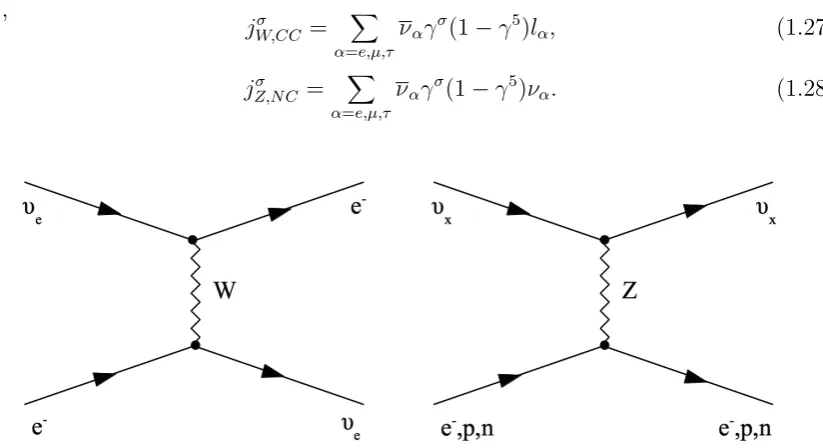
the sign of the mass-squared difference, thus depending on the mass hierarchy [26]. The are two types of neutrino interaction that occur with matter, Charged Current (CC) and Neutral Current (NC), these are shown in figure 1.1. The exchange of a charged W boson indicates a CC interaction, while a Z boson exchange indicates a NC interaction. These two processes can be expressed by the following leptonic currents [22],

j_W,CCσ = X

α=e,µ,τ

ναγσ(1−γ5)lα, (1.27)

j_{Z,N C}σ = X

α=e,µ,τ

ναγσ(1−γ5)να. (1.28)

Fig. 1.1 Feynman diagrams of coherent forward scattering processes, CC on the left and NC on the right.

The average effective Hamiltonian term, H(_effCC)(x), corresponding to the CC inter-actions in matter is

H_eff(CC)(x) =VCCνeL(x)γ0νeL(x). (1.29)

Where our CC potential term VCC is

VCC =

√

2GFNe (1.30)

with GF being the Fermi constant and Ne the electron density of the medium. The

NC contribution must consider all neutrino flavour interactions with protons, neutrons and electrons.

V_{N C}f =√2GFNfgfV (1.31)

[image:30.595.90.502.202.426.2]

(31)

1.4 The Neutrino 13

neutrality of atoms in matter these terms do not contribute and only the neutron term persists.

VN C =−

1

√

2GFNn (1.32)

With Nn as the neutron density of the medium. We then have

Vα =

√

2GF

Neδαe−

1 2Nn

, (1.33)

as our total potential. Now the Hamiltonian reads,

H=H0+H1 (1.34)

with our vacuum Hamiltonian term H0 and H1 arising due to the effective potential from matter effects. These matter effects are negligible in most practical cases as

GF/(~c)3 = 1.17×10−5 GeV−2, but over large enough distances through a medium,

where matter densities are high, these effects can be quite considerable. Indeed such vast distances do occur in the Sun and in proposed long baseline experiments such as LAGUNA-LBNO, with the aim to use these matter effects to probe the nature of neutrinos.

In the context of LAGUNA-LBNO, a muon (anti)neutrino beam is proposed. Both the appearance (νµ → νe) and disappearance (νµ → νµ) channels are examined to

include these matter effects. Implementing the 3 × 3 matrix the probability for the appearance transition can be approximated as equation 1.35 [27].

P(νµ →νe) = 4c213s 2 13s

2 23 1 +

2α

∆m2 31

(1−2s2₁₃)

!

sin2∆31

+ 8c2₁₃s12s13s23(c12c23cosδ−s12s13s23)cos∆32sin∆31sin∆21

−8c2₁₃c12c23s12s13s23sinδsin∆32sin∆31sin∆21

+ 4s2₁₂c2₁₃(c₁₂2 c2₂₃+s2₁₂s2₂₃s2₁₃−2c12c23s12s23s13cosδ)sin2∆21

−8c2₁₃s2₁₃s2₂₃αL

4Eν

(32)

14 Introduction

Wheres for disappearance transition probability is shown by equation 1.36 [23].

P(νµ→νµ) = 1−4s223c 2 13(c

2 12c

2 23+s

2 12s

2 13s

2

23−2c12c23s12s13s23cosδ)sin2∆23

−4s2₂₃c2₁₃(s2₁₂c2₂₃+c2₁₂s₁₃2 s2₂₃+ 2c12c23s12s13s23cosδ)sin2∆13

−4(c2₁₂c2₂₃+s2₁₂s2₁₃s2₂₃−2c12c23s12s13s23cosδ)

×(s2₁₂c2₂₃+c2₁₂s2₁₃s2₂₃+ 2c12c23s12s13s23cosδ)sin2∆12 (1.36) Here ∆ij =

1.27∆m2

ij

eV2

L km

GeV

Eν . In the νe appearance channel matter effects have been

included with α = 2√2GfneEν = 7.56×10−5eV2_g/cmρ 3

Eν

GeV, where the density of the

earth is taken asρ= 2.8g/cm3_,_G

f is the Fermi constant andne is the electron density

[23] [27].

Examining the expressions for the probability, the baseline Land the energyE are the only free parameters. Optimisation of these values and hence of L/E, will result in a maximal probability for the desired channel.

1.4.4 Current Status

Current values for the 3 mixing angles and the mass difference oscillation parameters have been well established [28][29], shown in table 1.1.

Parameter Best Fit ± 1σ 2σ 3σ

∆m2 21[10

−5_eV2_] ₇_.₅₉+0.20

−0.18 7.24-7.99 7.09-8.19 ∆m2₃₁[10−3_eV2_{] (NH)} ₂_.₅₄_±₀_.₀₉ _2.28-2.64 _2.18-2.73 ∆m2

31[10

−3_eV2_{] (IH)} _-(2_.₃₄+0.10

−0.09) -(2.17-2.54) -(2.08-2.64) sin2_θ

12 0.312+0−0..017015 0.28-0.35 0.27-0.36 sin2_θ

23 0.51±0.06 0.41-0.61 0.39-0.64 sin2_θ

13 0.024±0.08 0.012-0.036 0.010-0.038

Table 1.1 The current neutrino oscillation parameters with best fit, 2σand 3σvalues, from [28], with the recent result from Daya Bay of θ13 [29].

Of the parameters in table 1.1 that which has been of most recent interest is

(33)

1.4 The Neutrino 15

sin2₂_θ

13= 0.103±0.013(stat)±0.011(syst) [31]. These combined efforts to determine

θ13 have shown that this parameter is no longer of key interest to future experiments and focus can be moved onto the remaining undetermined parameters, δCP and the

sign of ∆m2₃₁.

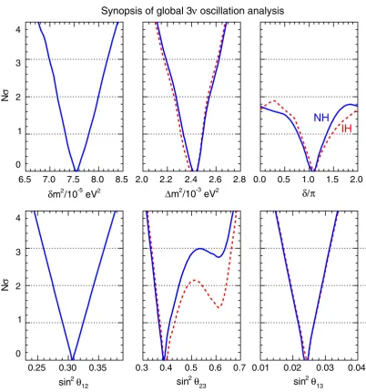
Current global analysis of the six independent parameters, sin2θ12, sin2θ13, sin2θ23,

δm2 ≡∆m2₂₁, ∆m2 ≡m2₃−(m2₁+m2₂)/2 (+∆m2 for NH and -∆m2for IH) andδCP are

shown with their corresponding N σ bounds in figure 1.2 [32]. The constraints of the parameters sin2_θ

13 and δCP can be seen in figure 1.3 when examining the combination

of Long Baseline (LBL) accelerator experiments, Solar experiments, KamLAND, and Short Baseline (SBL) reactor experiments and Atmospheric detectors.

1.4.5 CP Violation

From the MNSP mixing matrix there then remains one unknown parameter, the CP-violating phase, δ, which can now be determined as the mixing angle θ13 is shown to be non zero (or integer multiples of π) to larger than 5σ. The measurement of a large

θ13 was crucial for probingδCP as it is coupled with sinθ13in the MNSP. By comparing neutrino with anti-neutrino beams in Positive Focusing (PF) and Negative Focusing (NF) run modes respectively, asymmetries in their oscillation amplitudes will show a direct observation of CP Violation (CPV) in the leptonic sector. One can define the CP asymmetry as equation 1.37.

ACP_αβ =P(να →νβ)−P(να →νβ) (1.37)

1.4.6 The Mass Hierarchy

It is clear from looking at the oscillation probabilities that they depend on ∆m2 ij but

the problem lies in the sign of these. Is m2

3 > m21? This is a question that remains unresolved. In a vacuum these probabilities cannot discriminate between the sign as they arise in sine and cosine terms which cancel out the sign effects. However with the inclusion of the effective matter potential and the MSW effect, terms arise in the oscillation probability to make it possible to observe this sign. It is well established that ∆m2₂₁is positive [33]. This is due to matter effects of the Sun. The mass hierarchy problem is the problem of resolving the sign of ∆m2

(34)

16 Introduction

(especially in NH), a possible hint in favor of

!

_!

"

(mainly from SK atm. data), and no hint about the mass

hierarchy.

IV. SUMMARY OF OSCILLATION CONSTRAINTS

AND IMPLICATIONS FOR ABSOLUTE MASSES

In this section we summarize the previous results in

terms of one-parameter constraints, all the others being

marginalized away. We also show updated oscillation

con-straints on the main absolute mass observables [

44 ,

45 ],

namely, the effective electron neutrino mass

m

_#

(probed in

#

decay), the effective Majorana mass (probed in

0 $

2 #

decay searches), and the sum of neutrino masses

!

, which

can be probed by precision cosmology.

Figure

3 shows the

N

%

bounds on the

3 $

oscillation

parameters. Blue (solid) and red (dashed) curves refer to

NH and IH, respectively. The curves are expected to be

linear and symmetric around the best fit only for Gaussian

uncertainties. This is nearly the case for the squared mass

differences

!

m

2

_and

_"m

2

_{, and for the mixing parameters}

sin

2

&

12

and

sin

2

&

13

. The bounds on

sin

2

&

23

are rather

skewed towards the first octant, which is preferred at

&

2 %

in NH and

&

3 %

in IH. Also the probability distribution

of

!

is highly non-Gaussian, with some preference for

!

close to

"

, but no constraint above

_!

2 %

. As expected,

there are no visible differences between the NH and IH

curves for the parameters

!

m

2

and

sin

2

&

12

, and only minor

variations for the parameters

"m

2

and

sin

2

&

13

. More

pro-nounced (but

&

1 %

_Þ

differences between NH and IH

curves can be seen for

sin

2

_&

23

and, to some extent, for

!

.

Table

I

reports the bounds shown in Fig.

3 in numerical

form. Except for

!

, the oscillation parameters are

con-strained with significant accuracy. If we define the average

1 %

fractional accuracy as

1 =

6 th of the

#

3 %

variations

around the best fit, then the parameters are globally

deter-mined with the following relative precision (in percent):

!

m

2

_(2.6%),

_"m

2

_(3.0%),

_sin

2

_&

12

(5.4%),

sin

2

&

13

(10%),

and

sin

2

&

23

(14%).

A final remark is in order. As noted in Sec.

II B

, two

alternative choices were used in [

5 ] for the absolute reactor

flux normalization, named as ‘‘old’’ and ‘‘new,’’ the latter

being motivated by revised flux calculations. Constraints

were shown in [

5 ] for both old and new normalization,

resulting in somewhat different values of

&

12

and

&

13

. The

precise near/far data ratio constraints from Daya Bay [

6 ,

8 ]

and RENO [

7 ,

9 ] are largely independent of such

normal-ization issues, which persists only for the reactor data

12 θ 2 sin 0 1 2 3 4 23 θ 2

sin _sin2θ₁₃

2 eV -5 /10 2 m δ 0 1 2 3 4 2 eV -3 /10 2 m

∆ δ/π

0.25 0.30 0.35 0.3 0.4 0.5 0.6 0.7 0.01 0.02 0.03 0.04

6.5 7.0 7.5 8.0 8.5 2.0 2.2 2.4 2.6 2.8 0.0 0.5 1.0 1.5 2.0

oscillation analysis

ν

Synopsis of global 3

σ N σ N NH IH

FIG. 3 (color online). Results of the global analysis in terms of N%bounds on the six parameters governing 3$oscillations. Blue

(solid) and red (dashed) curves refer to NH and IH, respectively.

G. L. FOGLIet al. PHYSICAL REVIEW D 86, 013012 (2012)

013012-6

Fig. 1.2 The six parameters, sin2θ12, sin2θ13, sin2θ23,δm2 ≡∆m221, ∆m2 ≡m23−(m21+

m2

2)/2 (+∆m2 for NH and -∆m2 for IH) and δCP are shown from a global analysis

[image:34.595.87.490.166.597.2]

(35)

1.4 The Neutrino 17

normal hierarchy), with a combined statistical significance &3!in NH and&2!in IH.

Figure 2shows the results of the analysis in the plane

(sin2_"

13;#). The conventions used are the same as in Fig.1.

Since the boundary values#=$¼0and 2 are physically

equivalent, each panel could be ideally ‘‘curled’’ by smoothly joining the upper and lower boundaries.

In the left panels, constraints onsin2_"

13are placed both

by solarþKamLAND data (independently of #) and by

current LBL accelerator data (somewhat sensitive to #).

Once more, it can be noted that larger values of "13 are

allowed in IH. The best fit points are not statistically

relevant, since all values of # provide almost equally

good fits at#1!level. The ‘‘fuzziness’’ of the1!contours

is a consequence of the statistical degeneracy of the two

solutions allowed at 1! in Fig. 1, and which involve

complementary values of"23and somewhat different

val-ues of"13. At1!, the fit is ‘‘undecided’’ between the wavy bands at smaller and larger values of"₁₃, and easily flips

between them. At 2 or3!the two bands merge and such

degeneracy effects are no longer apparent.

In the middle panels, SBL reactor data pick up a very

narrow range of"13and suppress degeneracy effects. Some

sensitivity to#starts to emerge, since the ‘‘wiggles’’ of the

bands in the left panel best match the#-independent SBL

reactor constraints onsin2_"

13 only in certain ranges of#.

The match is generally easier in inverted hierarchy (where

LBL data allow a larger"₁₃range) than normal hierarchy.

In the right panels, atmospheric neutrino data induce a

preference for #_#$, although all values of # are still

allowed at#2!. Such a preference is consistent with our

previous analyses limited tocos#¼ $1 [4,5], where we

found #_¼$ preferred over #_¼0, in both normal and

inverted hierarchy. As discussed in [4], for #_#$ the

interference term in the oscillation probability provide some extra electron appearance in the sub-GeV atmos-pheric neutrino data, which helps fitting the slight excess of electronlike events in this sample. In our opinion, atmospheric data can provide valuable indications about

the phase#, which may warrant dedicated analyses by the

SK experimental collaboration, especially in combination with data from the T2K collaboration, which uses SK as far detector and thus shares some systematics related to final state reconstruction and analysis.

Concerning the hierarchy, in the middle panels of

Figs. 1 and 2 (all data but SK atm.) we find a slight

preference for IH with respect to NH (!%2_’_%₀_:₃₈_{). The}

situation is reversed in the right panels (all data, including

SK atm.), where NH is slightly favored (!%2_’_þ₀_:₃₅_).

These fluctuations between NH and IH fits are statistically irrelevant. We conclude that, in our analysis of oscillation data, there are converging hints in favor of "₂₃<$=4

0.00 0.02 0.04 0.06 0.5

1.0 1.5 2.0

0.00 0.02 0.04 0.06 0.5

1.0 1.5 2.0

0.00 0.02 0.04 0.06 0.5

1.0 1.5 2.0 0.00 0.02 0.04 0.06

0.5 1.0 1.5 2.0

0.00 0.02 0.04 0.06 0.5

1.0 1.5 2.0

0.00 0.02 0.04 0.06 0.5 1.0 1.5 2.0 σ 1 σ 2 σ 3 13 θ 2

sin _sin2θ₁₃

13 θ 2 sin 13 θ 2

sin _sin2θ₁₃

13

θ

2

sin LBL + Solar + KamLAND + SBL Reactors + SK Atm

π

/

δ π/δ π/δ

π

/

δ π/δ π/δ

IH IH IH

NH NH NH

FIG. 2 (color online). Results of the analysis in the plane charted by_ðsin2_"

13;#Þ, all other parameters being marginalized away. From

left to right, the regions allowed at 1, 2 and3!refer to increasingly rich data sets:LBL_þsolar_þKamLAND data (left panels), plus SBL reactor data (middle panels), plus SK atmospheric data (right panels). A preference emerges for#values around$in both normal hierarchy (NH, upper panels) and inverted hierarchy (IH, lower panels).

GLOBAL ANALYSIS OF NEUTRINO MASSES, MIXINGS,. . . PHYSICAL REVIEW D86,013012 (2012)

013012-5

Fig. 1.3 Global results in the plane of sin2_θ

13 and δCP. The left plots show analysis

(36)

18 Introduction

Fig. 1.4 The mass hierarchy of neutrinos, the normal hierarchy (NH) on the top and the inverted hierarchy (IH) on the bottom. This graphic shows the larger the circle the larger the value of m2_i.

1.4.7 Sterile Neutrinos

Neutrinos could in theory oscillate to other flavours that do not interact weakly, un-like the 3 flavours we currently observe. This would then alter observed oscillation probabilities and could give an indirect indication to such a family of neutrinos. These particular variety of theorised neutrinos are named sterile neutrinos and as of yet are to be experimentally confirmed.

1.4.8 Neutrino Interactions

Neutrinos can only interact in one way (ignoring gravity), that is, weakly. These interactions are well described processes in the Standard Model. Although neutrino oscillations are not described in the Standard Model, there have been no experimen-tally observed deviations from the Standard Model for neutrino interactions. Of course oscillations imply neutrino mass, and the Standard Model does not account for this but with neutrino mass limitmνe< 2.3 eV/c

2 _{at 95% confidence [34], the kinematic} ef-fects of this small mass are negligible for oscillation experiments and are only relevant for mass measurement experiments.

(37)

1.4 The Neutrino 19

to be well understood. LAGUNA-LBNO and most long baseline experiments are concerned in the intermediate energy scale of 0.1 to 100 GeV [35]. In this energy range several important physical process contribute. There are three main neutrino interactions concerning this intermediate energy scale. They consist of Elastic/Quasi-Elastic (E/QE), Resonance (RES) and Deep Inelastic Scattering (DIS) interactions.

Elastic and Quasi Elastic: Considered the simplest and most well understood interaction type in detectors, elastic scattering occurs with an electron or a nucleon. In either of these cases however it impossible to detect the final state neutrino in the detector and only the lepton/nucleon can be seen.

QE interactions are not elastic but considered semi elastic due to low momentum transfer. They involve the production of new particles in the final state if above the production threshold. Charge Current Quasi Elastic (CCQE) interactions are prevalent below the ∼1 GeV regime, with neutrino-nucleon scatterings of

νl+n→p+l−, (1.38)

νl+p→n+l+, (1.39)

where l represents the charged lepton, l =e, µ, τ, and interacting with the proton, p, or the neutron, n in the nucleon. In practice only electron and muon (anti)neutrinos are feasible with tau neutrino beams originating from astrophysical events. CCQE interactions are favourable in experiments as the neutrino energy can be solely recon-structed from the momentum of the lepton, by conservation of momentum and energy we have

Eνl =

ElmNc2−m2lc4/2

mNc2−El+plccosθ

. (1.40)

Here Eνl and El are the energies of the neutrino and lepton respectively,mN denotes

the mass of the proton or neutron (depending on neutrino or antineutrino case). The transverse momentum of the charged lepton is given by pl, with the angle between

the lepton and the incident neutrino as θ. Determination of the angle cannot be done from the lepton alone and without accurate measurement of the final state nucleons momentum it is assumed that angle is taken with respect to the beam axis.

Resonance: In the region between elastic and inelastic processes, around 1 GeV, RES events are common. Through the excitation of baryon resonances pions are produced via,

(−)

νl +N →l±+N∗, (1.41)

(38)

20 Introduction

Fig. 1.5 CCQE interaction at tree level.

then decays with pions in the final state.

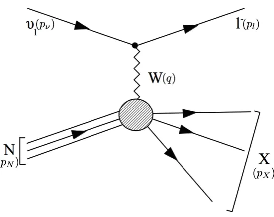
Deep Inelastic Scattering: When neutrino energies are high enough that they well exceed the proton/neutron mass, Eν >> mN, DIS interactions dominate. These

processes are defined as

(−)

νl +N →l±+X, (1.42)

with N = proton or neutron and X represents a set of final state hadrons. Such interactions are notoriously difficult to fully reconstruct in detectors as they usually results in high multiplicities. Determining cross sections of such events require the use of structure functions, Fi(x, Q2) which are given in terms of two Lorentz invariants,

x≡Q2_/₂_p

N ·q and Q2 ≡ −q2 [22].

Quantum ChromoDynamics (QCD) and nuclear effects make understanding neu-trino interactions difficult. Neuneu-trinos can interact on the atomic scale, nuclear scale or quark scale. Due to the non perturbative nature of these interactions several models are used to describe the various interaction processes. Current experimental mea-surements of neutrino cross sections are not well known in the low GeV range, with several different models and calculations driving most oscillation measurements. These current measurements are shown in figure 1.8 [35].

1.4.9 Types of Neutrino Experiment

(39)

1.4 The Neutrino 21

Fig. 1.6 RES interaction with single pion production at tree level.

[image:39.595.172.441.138.347.2] [image:39.595.169.445.455.673.2]

(40)

22 Introduction

[image:40.595.138.429.170.600.2]

(41)

1.4 The Neutrino 23

sensitivity of ∆m2_{, which is defined as equation 1.43 [22]. The longest baseline is} described first, that is neutrino experiments using the Sun as their source.

∆m2 ∼ 2E[GeV]

L[km] (1.43)

1.4.9.1 Solar Neutrino Experiments

The Sun is a rich and powerful source of electron neutrinos due to fierce fusion processes in its core. Copious amounts of neutrinos at energies of several MeV are produced, but consist of only electron flavour, arising from reactions shown in figure 1.9. Large amounts of these neutrinos are produced with a neutrino flux of about 6 × 1010 cm−2_s−1 _{on the Earths surface [22]. The predicted neutrino flux emitted from the Sun} as a function of energy is shown in figure 1.10.

Fig. 1.9 The fusion reactions that occur in the sun. Process chain based on [22].

[image:41.595.165.443.358.589.2]

(42)

24 Introduction

Fig. 1.10 The neutrino flux from the solar fusion processes. The percentages indicate the uncertainties in the values. Figure taken from [36].

Neutrino problem by measuring CC interactions for the νe rate and NC interactions

to yield the total ν rate.

The distance between the Sun and the Earth is approximately 1.5 ×1011_{m. With} the energy spectrum ranging between 0.1 - 15 MeV this gives an upper bound of L/E

∼1012 _{m/MeV, corresponding to a sensitivity of ∆m}2 _∼₁₀−12 _eV2_{. Although with the} radius of the Sun at roughly 7×108 _{m they can experience considerable matter effects} inside the Sun before reaching the surface.

1.4.9.2 Atmospheric Neutrino Experiments

[image:42.595.155.421.112.325.2]

(43)

1.4 The Neutrino 25

a wide range of energies varying from 500 MeV to 100 GeV.

π±→µ±+(ν−µ) (1.44)

µ− →e−+νe+νµ (1.45)

µ+ →e++νe+νµ (1.46)

Measurements using atmospheric neutrinos require different techniques than solar ex-periments as they no longer originate from one localised source. As neutrinos can originate from anywhere in the atmosphere then directional information is key in studying these neutrinos.

With distances varying dramatically depending on the several atmospheric levels, the baseline is anywhere between 10 - 10,000 km. Taking the lower bound gives a sensitivity of ∆m2 _∼₁₀−4 _eV2_{. Kamiokande [37] and IMB [43] are two experiments} that have measured atmospheric neutrinos.

ATMOSPHERIC NEUTRINOS

391

¯

νµ

νµ ν¯µ

π+ π−

νµ e− ¯ νe νe µ+ µ− e+ p

Fig. 11.1.

Schematic view of

neu-trino production by cosmic-ray

proton interactions in the

atmo-sphere, with generation of pions

and muons.

0 1 2 3 4 5 0 0.005 0.01 0.015 sub GeV multi GeV stopping muons through-going muons

10-1 100 101 102 103 104 105

E , GeV

dN/dlnE, (Kt.yr)

-1

(m .yr.ster)

2

-1

Fig. 11.2.

Distributions of neutrino

ener-gies that give rise to four classes of

events [489]. Sub-GeV and multi-GeV

refer to contained events in Kamiokande

and Super-Kamiokande. Stopping and

through-going muons refer to

neutrino-in-duced muons proneutrino-in-duced outside the

detec-tor.

and in the East Rand Proprietary Gold Mine in South Africa [900]. Both

experi-ments were located very deep underground, with overburdens of about 8000 mwe

60

.

The detectors were made of scintillator, which recorded the tracks of muons. Deep

underground the residual secondary cosmic-ray muon flux is strongly peaked in the

downward-going vertical direction. On the other hand, the atmospheric neutrino

flux is almost isotropic and can generate upward-going and horizontal muons by

interacting with the rock surrounding the detector. Nowadays detectors can

distin-guish upward-going muons from the downward-going secondary cosmic-ray muons,

but at that time it was only possible to reveal the atmospheric neutrino flux by

measuring horizontal muons. The events reported by the Indian and South-African

experiments were of horizontal type, with a very low probability of being generated

by cosmic-ray muons. In the following years, the observation with scintillator

detec-tors of muons generated in the rock by atmospheric neutrinos continued in India

[704, 705], in South Africa [901, 341], in Utah (USA) [211], and in the Baksan

Laboratory in Russia [260, 261, 65].

In the second half of the 1980s, atmospheric neutrinos began to be observed by

the large underground Kamiokande [614, 840, 621, 474, 603] and IMB [581, 243, 306,

199, 200, 322] water Cherenkov experiments, which have been built for the search

of nucleon decay. These detectors could observe events generated by atmospheric

neutrino interactions in the detector, as well as upward-going muons generated

by atmospheric neutrino interactions in the rock below the detector. Initially, the

interactions of atmospheric neutrinos in the detectors were mainly considered as a

60

_{For an explanation of mwe units, see footnote 54 on page 367.}

[image:43.595.181.440.415.648.2]

(44)

26 Introduction

1.4.9.3 Reactor Neutrino Experiments

Fission reactors are another powerful source of neutrinos, producing electron antineu-trinos in large amounts ∼2 × 1020 _s−1_{. Arising from the} _β_{-decay of fission products} from reactions between 235_U, 238_U, 239_{Pu and} 241_{Pu they have typical energies of the} order of several MeV. Such energies result in shorter baselines but considering the isotropic nature of the flux this is beneficial for experiments using reactor neutrinos as a source. Only disappearance experiments are feasible as such energies are not sufficient to produce µ’s or τ’s in a detector through CC interactions. The common method to detect reactor neutrinos is via inverse beta decay.

Reactor neutrino experiments can be short or long baseline, with sensitivities of ∆m2 ∼0.1 eV2 _{and ∆}_m2 _∼₁₀−3 _eV2 _{respectively. Experiments that employ this} method are Daya Bay[44], RENO[45] and CHOOZ[46].

1.4.9.4 Accelerator Long Baseline Experiments

Neutral particle detection methods using Noble gases in LAGUNA-LBNO and MODES-SNM