This is a repository copy of A study on network design problems for multi-modal networks
by probit-based stochastic user equilibrium .
White Rose Research Online URL for this paper:
http://eprints.whiterose.ac.uk/2479/
Article:
Uchida, K., Sumalee, A., Watling, D.P. et al. (1 more author) (2006) A study on network
design problems for multi-modal networks by probit-based stochastic user equilibrium.
Networks and Spatial Economics, Online. ISSN 1572-9427
DOI:10.1007/s11067-006-9010-7
[email protected] https://eprints.whiterose.ac.uk/
Reuse
See Attached
Takedown
If you consider content in White Rose Research Online to be in breach of UK law, please notify us by
White Rose Research Online
http://eprints.whiterose.ac.uk/
Institute of Transport Studies
University of Leeds
This is an author produced version of a paper originally published in Networks
and Spatial Economics. It has been peer reviewed, but does not include the final
publisher’s pagination and formatting. The original publication is available at
www.springerlink.com.
White Rose Repository URL for this paper:
http://eprints.whiterose.ac.uk/
2479/
Published paper
Uchida K., Sumalee A., Watling, D.P., Connors, R.D. (2006)
A Study on Network
Design Problems for Multi-modal Networks by Probit-based Stochastic User
Equilibrium
- Networks and Spatial Economics online
A Study on Network Design Problems for Multi-modal Networks by
Probit-based Stochastic User Equilibrium
Kenetsu Uchida a, Agachai Sumalee b*, David Watling b, Richard Connors b
a Graduate School of Engineering, Hokkaido University
b Institute for Transport Studies, University of Leeds
* Corresponding author. 36 University Road, Leeds, LS2 9JT, UK Tel: +44-113-343-5345;
Fax: +44-113-343-5334.
Abstract. This paper develops a multi-modal transport network model considering various
travel modes including railway, bus, auto, and walking. Travellers are assumed to choose
their multi-modal routes so as to minimise their perceived disutilities of travel following the
Probit Stochastic User Equilibrium (SUE) condition. Factors influencing the disutility of a
multi-modal route include actual travel times, discomfort on transit systems, expected waiting
times, fares, and constants specific to transport modes. The paper then deals with the
multi-modal network design problem (NDP). The paper employs the method of sensitivity analysis
to define linear approximation functions between the Probit SUE link flows and the design
parameters, which are then used as constraints in the sub-problem of the NDP instead of the
original SUE condition. Based on this reformulated NDP, an efficient algorithm for solving
the problem is proposed in the paper. Two instances of this general NDP formulation are then
presented in the paper: the optimal frequency design problem for public transport services
LIST OF TABLES AND FIGURES
TABLE 1 Coefficients of link disutility.
TABLE 2 Coefficients of line disutility.
FIG. 1 Network representation for the transit network.
FIG. 2 Effects from dispersion of anti-freezing admixture.
FIG. 3 Link capacity as a function of the amount of anti-freezing admixture dispersion.
FIG. 4 Network representations for the multi-modal network.
FIG. 5 Modal shares of passengers between O1D1 for FDP.
FIG. 6 Surface of the objective function for the FDP.
FIG. 7 Contours of the objective function and trajectory of the optimization process for the FDP.
FIG. 8 Modal shares of passengers between O1D1 in summer and winter seasona.
FIG. 9 Modal shares of passengers between O1D1 for the AADP.
FIG. 10 Surface of the objective function for the AADP.
1. Introduction
The improvement or modification of a transport network and service often requires a
high level of investment. With limited public funds, it is important to carefully evaluate the
costs and potential benefits of different transport schemes. Transport network models have
long been used as a decision support system for the decision-maker in evaluating potential
benefits and impacts of different transport projects. This is one way of using a model, as an ad
hoc tool.
It is also possible to use the model to directly identify the best (optimal) way to
modify the transport network/service. This problem is widely referred to as the Network
Design Problem (NDP). The NDP for the case of automobile-only networks has been widely
studied in the literature (see for example Abdulaal and LeBlanc 1979; Tobin and Friesz 1988;
Yang and Bell 1997; Shepherd and Sumalee 2004). The NDP is normally formulated as a
Mathematical Program with Equilibrium Constraints (MPEC) in which the planner aims to
define modifications to a network so as to optimise an objective function, whilst considering
the response of travellers to the changes following an equilibrium condition. Often, the
travellers’ responses are assumed to follow Wardrop’s User Equilibrium condition (UE).
The NDP is not only applicable to the case of the road network. It can also be used to
analyse transit network planning or in a more general multi-modal network case. Note that
public transport users are believed to be more strategic (than those in an automobile network)
in choosing their routes or service lines, depending on the arrival of services at the boarding
point or the expected waiting time (Chiriqui and Robillard 1975). At the tactical level, the
design parameters involved in the NDP of the transit network may include service line,
service frequency and fare level and structure. Most of the works reported in the literature
related to the NDP of a transit network simply ignore the response of travellers to the change
or configuration of the transit network or service (Gao et al 2004).
Gao et al (2004) pointed out this pitfall of previous studies and proposed a
formulation of a continuous NDP of transit systems with the UE model for transit network
proposed in De Cea and Fernandez (1993), an extension of the model proposed by Spiess and
Florian (1989) to consider the impact on waiting delay of limited vehicle capacities. In this
paper we aim to apply the NDP with a more advanced framework of the multi-modal network
as compared to the one adopted in Gao et al (2004). In this respect, the main improvements in
the model adopted for the NDP in this paper are fourfold.
First, we extend the analysis of the NDP to the case of a multi-modal network in
which a single journey may comprise more than one mode (see e.g. Fernandez et al 1994; Lo
et al 2003). Second, the model adopted in this paper allows some public transport modes to
share the road space with the private automobile. Thus, their travel times on the road network
are interrelated with traffic volumes and vice versa. This is particularly important for the
optimal frequency design problem since a large increase in bus frequency may ultimately
cause some major travel delays on some links. Third, we introduce an in-vehicle “congestion
effect” in addition to the waiting time. This is mainly to represent the discomfort or crowding
effect on public transport passengers, which may influence travellers’ behaviour (Kraus
1991). Similar to the model proposed in this paper, Kurauchi et al (2003) propose a transit
assignment model with a nonlinear crowding effect.
Lastly, the framework of probit Stochastic User Equilibrium (SUE) is adopted instead
of UE. The concept of SUE is believed to be a more plausible model than UE in allowing for
mis-perceptions and uncertainties in travellers’ predictions of travel disutilities. It has also
been shown that it can eliminate some problems in solving the NDP caused by the UE
condition (Lawphongpanich and Hearn 2004; Sumalee et al 2005). Several previous
researchers have also applied SUE to the case of a public transport network model. Lam et al
(1999) introduced line capacity constraints to a logit-based SUE transit assignment for a
congested transit network. Lo et al (2003) also adopted the logit SUE model to represent
passengers’ route choice behaviours. Nielsen (2000) presented a framework for transit
assignment that builds on a probit-based SUE model that resolves the problem with
overlapping routes in the logit-model, caused by its IIA (independence of irrelevant
Apart from these four improvements to the multi-modal model in the NDP context,
this paper also presents a new application of the NDP with the optimal anti-freezing
admixture dispersion problem, in addition to the optimal frequency design problem. The
paper is structured into seven further sections.
The next section introduces the representation of a multi-modal network. Then in
Section 3, the probit-based SUE formulation for passengers’ route choice in the multi-modal
network is explained. This section also gives details of the definition and formulation of the
different components of disutility of travel on a multi-modal route. Two network design
problems of optimal transit frequency design (FDP) and optimal anti-freezing admixture
dispersion (AADP) are formulated in Section 5. Then, Section 6 proposes a solution
algorithm for the NDP. Section 7 then discusses the numerical examples and Section 8
concludes the paper and discusses future research needs.
2. Network Representation
First, some definitions will be made in order to explain the network representation. A
transit line (or just a line) is a group of vehicles that runs back and forth between two nodes
on a transit network. A line section is any portion of a transit line between two (not
necessarily consecutive) nodes of its itinerary. Figure 1a shows a simple example of the
primitive network taken from Spiess and Florian (1983). There are four lines in this network
(L1-L4). This primitive network is transformed into a modified network shown in Figure 1b,
i.e.G(N,S) with node set N representing transit stops and link set S representing route
sections. A route section is a portion of a route between two consecutive transfer nodes. A
route is any path that a transit user can follow on the transit network to travel between any
two nodes. In Figure 1b, each route section is associated with a set of attractive lines
characterizing expected travel time on that route section. The set of attractive lines on route
{ }
∑
∑
+
=
l s l l l
s l l s l s
x
f
x
x
f
t
Z
s l
α
60
min
(1)s.t.
∑
= ∈
∀ =
l s l l s s s
l l A f f x
x 0 ,1 ,
,
(2)where, As
,
fl and tls denote a set of all transit lines passing through route section s, thefrequency of transit line l (services/hr) and the constant in-vehicle travel time (min.) of route
section s using transit line l respectively. The objective function as defined in Eq.(1) denotes
the total expected travel time, i.e. the expected waiting time plus the expected in-vehicle
travel time, calculated using frequencies and constant in-vehicle travel times of transit lines
on route section s. The effect of both the distribution of headway times of the transit lines and
the distribution of passenger arrival times on the calculation of the expected waiting time is
captured by the parameter in Eq.(1).
[INSERT FIGURE 1]
The case = 1 corresponds to an exponential distribution of interval times of the
transit lines with mean 1/fs and a uniform passenger arrival rate. The case = 1/2 is an
approximation of a constant headway time 1/ fs for the transit lines. A line l∈As will be
included in a set of attractive lines (As) for route section s if xls =1, and will not be
considered as a possible line ifxls =0.
In this paper, the multi-modal network is expressed as a hyper-network, i.e. the road
network including the walking network plus the modified network representing the transit
network as mentioned above. Links for auto or walking can be considered as links used by the
L+1th dummy line where L denotes the number of real lines in the multi-modal network with
frequencies and service capacities of infinity, i.e. a waiting time and in-vehicle discomfort of
zero. Based on this idea, we will denote transit stops and route sections as nodes and links
Fig. 1. Network representation for the transit network. L1
A
L2 L2L3 L3
L4
x
y
B
(a) Primitive network and its itinerary.
Lines Itineraries L1 A -> B L2 A -> x -> y L3 x -> y -> B L4 y -> B
S1 (L1)
A
S2 (L2) S3 (L2, L3) S4 (L3, L4)
S6 (L3)
x
y
B
Ss (attractive lines)
autos and buses may share the same road space and this is represented in the hyper-network
by using two different links having interactions with each other in terms of the congestion
effect. However, the delay on the pseudo-link representing a bus line also includes the
in-vehicle congestion effect (expected waiting time). The link set of the hyper-network will be
comprised of four subsets associated with the four transport modes.
m u b a w
m S
S
} , , , {
∈ ∪
=
where m indicates transport modes for walking (m=w), auto (m=a), bus (m=b) and subway
(m=u), and Smindicates a set of links in which the transport mode is m. Henceforth, we will
denote by s an element of the set S when we do not have to distinguish transport modes.
3. Link Disutility Functions
3.1. Notation
The notation adopted in this paper is shown below:
S The number of links comprising the multi-modal network. L The number of real lines in the multi-modal network
A (S × L+1)-matrix that has an element asl, representing the sth row and lth column of A; equal to 1 if link s includes a line l as one of its attractive lines, and 0 otherwise
s
A The set of lines that are included in link s as attractive lines
V S-vector of link flows, having sth element V s denoting the number of passengers on link s
v (S × L+1)-matrix that has an element vsl, representing the sth row and lth column of v, that denotes the number of passengers on link s using line l ( =
∑
l sl
s v
V ).
sl v
~ The number of passengers that share the same line l with the passengers on link s using line l (vsl)
s
V~ The number of passengers that share the same link with the passengers on link s (Vs), ( =
∑
∈ sA l sl s
v
V~ ~ )
f (L+1)-vector of line frequencies that has an element fl, representing the lth element of f, which denotes the frequency of line l (services/hr.)
(L+1)-vector of service capacities that has an element l, representing the lth element of , which denotes vehicle capacity comprising a service of the transit line l (passengers/service)
t* S-vector of actual travel times that has an element t*s, representing sth element of t*; equal to 0 if s∈Sb, and ts otherwise, where ts denotes actual travel time of link s
tˆ S-vector of perceived travel time that has entries
t
ˆ
srepresenting the sth element of tˆ, which denotes the perceived travel time of link s.w S-vector of link expected waiting time with ws representing expected waiting time of link s.
p S-vector of fares on links with entries ps representing the fare on link s.
(S × S)-matrix that has an element ss', representing the sth row and s'th column of ;
equal to 1 if in-vehicle congestion on link s is affected by the number of passengers on link s', and 0 otherwise
J (S × L+1)-matrix that has an element jsl, representing the sth row and lth column of J; equal to 1 if link s is a direct link regarding line l, and 0 otherwise, where if the passengers travelling on link s using line l cannot alight from the line along the way, we call link s a direct link regarding line l
H (S × L+1)-matrix that has an element hsl, representing sth row and lth column of H; equal to 1 if line l passes through link s in the original network, and 0 otherwise for s∈Sa and l≠L+1; equal to 1 for s∈Sa∪Sw and l=L+1; equal to 0 for s∈Sw and
1 + ≠L
l ; equal to 0 for s∈Sb and ∀l; and equal to asl for s∈Su and ∀l
E (S × S) matrix that has an element ess', representing the sth row and s'th column of E;
equal to 1 if s = s', and 0 otherwise for s∈Sb; and equal to 1 if actual travelling time on link s is affected by the number of passengers on link s'∈Sa, i.e. equal to 1 in the case where bus link s shares auto link s' in the original network, and 0 otherwise
1S S-vector whose elements are all equal to 1 1L+1 (L+1)-vector whose elements are all equal to 1
In this paper, the arithmetic signs of ⊗ and ÷ indicate the special operations of
element-by-element multiplication and division for matrices or vectors, respectively. For
example, element-by-element multiplication of matrices of M and N is written as M⊗N in
which the element in the ith row and jth column of the matrix M⊗N is mij nij, where mij and
nij indicate the elements in the ith row and jth column of M and N respectively. The arithmetic
sign of ÷ indicates element-by-element division of matrices or vectors, such that M÷N has
an element in the ith row and jth column of mij /nij. Note that, two matrices (or vectors) used for
two arithmetic signs of ⊗ and ÷ should have the same size. The superscript T denotes the
conventional matrix transposition operator.
3.2 Disutility of link and intermodal route
In this paper, the travellers are assumed to consider four main components of the
inconvenience or disutility of travel on a link or route, explicitly including travel time,
in-vehicle congestion effect, expected waiting time, and fares. As we will explain later in the
combined as a perceived travel time. Thus, in general the total disutility of using hyper link s
in the intermodal network as described in the previous section can be defined as:
p
w
t
d
=
⊗
ˆ
+
⊗
+
⊗
, (3)s
p
w
t
d
s=
π
sˆ
s+
ρ
s s+
τ
s s∀
, (4), following the notation defined in the previous section, where , , and denote coefficients
vectors (all with the size of S ×1) on the perceived travel times vector, waiting times vector
and fares vector, respectively
Then, the disutility function of an intermodal route can be defined as the sum of the
related link disutilities with an additional term of a mode specific constant (or alternative
specific constant, ASC). The disutility of the kth intermodal route connecting origin node r
and destination node s, i.e. the kth intermodal route between OD pair rs, is given by:
rs
K
k
d
du
srsk rsS s
s
u b a w m
rs k m m rs
k
=
∑
+
∑
∀
∈
∀
∈ ∈
,
, }
, , , {
,
δ
ζ
α
, (5)where, mdenotes the mode specific constant for mode m. For a kth intermodal route between
OD pair rs
ζ
mrs,k= 1 if it
contains at least a link whose transport mode is m and δsrs,k=1 if it
is
related to link s. Otherwise,ζ
mrs,kor
δsrs,kis
0. The set of intermodal routes connecting ODpair rs is Krs. The monetary costs of auto are mainly due to car ownership costs, fuel costs,
and tolls. The car ownership cost is reflected by the mode-specific constant for auto.
It is noted that a number of previous studies have also considered the impact on the
disutility of a trip of modal transfers (see for example Lo et al , 2003). In the present study,
the disutility from the number of modal transfers will not be modelled explicitly, because it
can also be represented implicitly inside the expected waiting time and walking travel time.
As explained later in Section 3.4 and 3.5, the formulations of perceived in-vehicle
travel time (with the crowding effect) and the expected waiting time are functions of two
types of passenger flows. First, they are functions of the number of passengers already
on-board, which obviously influences the level of in-vehicle congestion for each service line and
passengers wishing to board and alight at different stations. The definitions and mathematical
formulation in matrix form will be explained next.
3.3 Formulation of passenger volumes
For the passenger volume using line l on link s (
v
sl) can be simply defined in amatrix format as:
) ( )) diag(
( ⊗ TL+1
= A f P1
v (6)
where ⎟ ⎟ ⎟ ⎠ ⎞ ⎜ ⎜ ⎜ ⎝ ⎛ = +1 1 0 0 ) diag( L f f L M O M L
f , (7)
{
}
⎟⎟ ⎟ ⎟ ⎟ ⎠ ⎞ ⎜⎜ ⎜ ⎜ ⎜ ⎝ ⎛ = ÷ ⊗ =∑
∑
∈ ∈ ) /( ) /( ) ( 1 1 1 s A l l S A l l f V f V M Af V P . (8)The element representing the sth row and lth column of v is given by:
l s f f V v s A l l l s
sl ⎟⎟ ∀ ∀
⎠ ⎞ ⎜⎜ ⎝ ⎛ =
∑
∈ , ''
.
(9)
This is simply based on the allocation of passenger volume on link s to each line in the set of
attractive lines (
l
∈
A
s) by their frequencies.The other part of the passenger volumes are those using or competing for the service
on line l that are associated with other links in the network. Following the structure of the
network representation discussed earlier, the service line may also be associated with different
links in the network apart from the link under consideration. In this case, we also have to
consider the passenger volumes on those links using the same service as the competing flows
or contributing flows to the line in-vehicle capacity and congestion respectively, the first term
passengers getting on board line l at the stop point of link s but using a different link in the
network, the second term on the right hand-side of Eq. (10) below. These two components of
passenger volumes can be combined together, defined as
v
~
sl:l
s
v
v
v
l s i l si r S r l S r r l
sl
=
∑
+
∑
∀
∀
∈ ∈ +
,
~
) ( ) (, (10)
where, i(s) is the origin node of link s, Sil(+s) indicates the set of links going out from node i(s),
but excluding a link s, that contains a line l∈As as an attractive line, and Sil(s) indicates the
set of links that contain a line l∈As as an attractive line, with origin node before i(s) and end
node after i(s).
In matrix form, using the notation introduced earlier, we can define the total
passenger volumes competing for or using the capacity of line l over link s as:
A v
C≡( )⊗ (11)
where C is a (S × L+1)-matrix with elements csl given by:
l
s
v
v
c
sl=
sl+
~
sl∀
,
∀
. (12)3.4 Formulation of perceived in-vehicle link travel time
In calculating the perceived in-vehicle travel time, we only need to evaluate the
values for the real physical links in the network. These links as included in the hyper-network
are the “direct links” defined in the notation section. For the road network and related bus
services, the actual travel time is assumed to follow a standard BPR function with an
interaction term between the bus and personal vehicle flows. Thus, the actual travel time,
t
s,
on road link s∈Sain the network can be defined as:
a s s pcu s l b l s s s S s K V E f t t s ∈ ∀ ⎥ ⎥ ⎦ ⎤ ⎢ ⎢ ⎣ ⎡ ⎪⎭ ⎪ ⎬ ⎫ ⎪⎩ ⎪ ⎨ ⎧ ⎟⎟ ⎠ ⎞ ⎜⎜ ⎝ ⎛ + + =
∑
∈ 1 ) ( ' ' γ ψβ
, (13)a a
a s s
pcu E s S
O V
V = ∀ ∈ , (14)
s
t andKsare the free-flow travel time (in minutes) and capacity (in pcus/hour) of link s∈Sa
respectively;ψ(s) is a set of bus lines passing through link s∈Sa in the original
network;Oais the average occupancy for auto (passengers / auto);EaandEbare passenger car
equivalents for auto and bus respectively; and
β
sandγ
sdenote calibration parameters.On the other hand, the actual travel times for underground (or separated transit
system) and walking links s∈Su ∪Sware constant, normally given a priori. The travel time
of bus links∈Sb corresponds to the actual travel time of link s for auto. As mentioned in the
previous section, the effect of travel and in-vehicle congestion is integrated into a single value
termed as perceived travel time. This will be discussed next.
Define a matrix G as:
{
}
[
⊗
1
÷
(
⊗
)
|
1>
0
,
1>
0
]
≡
T Tβ
γ
S
1
f
C
G
⎟ ⎟ ⎟ ⎠ ⎞ ⎜ ⎜ ⎜ ⎝ ⎛ ≡ + + 1 1 1 1 11 SL S L G G G G L M O M L
(15)
( )
(
)
( )
(
)
⎟⎟ ⎟ ⎟ ⎠ ⎞ ⎜⎜ ⎜ ⎜ ⎝ ⎛ = + + 1 1 1 1 1 1 1 1 1 1 1 11 1 γ γ γ γ β β β β SL S L g g g g L M O M L ,where the element gsl, as in Eq.(10), is the sth row and lth column of
{
}
T T S 1 fC⊗1÷( ⊗ ) ,
given by:
(
v
v
) (
f
)
s
l
g
sl=
sl+
~
sl lκ
l∀
,
∀
(16)Next, let us consider the following two matrices defined by Eqs.(17) and (18):
H J G E
Z≡{ T( ⊗ )}⊗ , (17)
H J E
Let zsl denote the element representing the sth row and lth column of matrix Z, the variable zsl
equals Gs'l' if line l is an attractive line of s∈Sb, and 0 otherwise. In this regard, any
combination of link and line, denoted (s', l'), must simultaneously satisfy the following two
conditions:
i) the actual travel time of link s∈Sb is affected by the actual travel time of link s'∈Sa,
in this case, actual travel times of link s and link s' are equal, or actual travel time of
link s is expressed as a summation of actual travel times of auto links including link
s'; and
ii) link s' is a direct link regarding line l'.
Accordingly, zsl is an index expressing the in-vehicle congestion effect of an
attractive line l over link s, and links for walking and auto are all equal to 0 by the definitions
of the two links. Let xsl denote the element representing the sth row and lth column of matrix X,
the variable xsl equals 1 if link s∈Sb is a direct link regarding line l, and 0 otherwise. The (S
× L+1) matrix ~t that expresses perceived travel times on line l over link s is given by:
{
t X Z}
At = ( + ) ⊗
~
,
(19)by using a matrix defined by Eq.(20).
) ( diag t* E
t≡ . (20)
The element t~lsdenoting the sth row and lth column of ~t , i.e. perceived travel time on line l
over link s, is given by:
l
s
f
v
v
t
z
t
t
l l sl sl l s s s sl l s s s s l∀
∀
⎪⎭
⎪
⎬
⎫
⎪⎩
⎪
⎨
⎧
⎟⎟
⎠
⎞
⎜⎜
⎝
⎛
+
+
⎟⎟
⎠
⎞
⎜⎜
⎝
⎛
=
+
⎟⎟
⎠
⎞
⎜⎜
⎝
⎛
=
∑
∑
∈ ∈,
~
1
)
1
(
~
1 1 ) , ( ' ' ) , ( ' ' γ θ θκ
β
(21)where 1 and 1 are calibration parameters on in-vehicle congestion; and (s, l) denotes a set
of direct links with respect to line l that are included in the set of attractive lines l∈As over
link s. Perceived travel time is expressed by the in-vehicle congestion effect, i.e. a discomfort
time (Fernandez et al 1994; Nielsen 2000). The S-vector that expresses link perceived travel
times is:
{
}
[
]
T) ( 1 ) ~ (
ˆ tf Af
t= ⊗ ÷ . (22)
Let tˆ denote the ss th element of tˆ , then tˆ is given by: s
s ~
ˆ =
∑
∑
∀∈
∈ s s
A l
l A
l l s l
s t f f
t . (23)
3.5 Formulation of the waiting time
The formulations of the waiting times for bus and underground services follow the
concept of an in-vehicle perceived travel time in which we have to consider both the number
of passengers already on board and those waiting to board at link s. The waiting time for
passengers waiting to board at link s will then be a function of the number of passengers on
related service lines boarding before link s and remaining in the vehicle after link s, and the
number of passengers waiting to get on board at link s itself. The first term is V~s as defined
earlier, and the second term is simply Vs. Following De Cea and Fernandez (1993), we define
a vector function as:
{
}
[
(C1 1) 1 (Adiag(f) ) |β2,γ2]
Q L+ ⊗ ÷
(
S)
TQ Q1 L
≡
( )
( )
TS q
q ⎟
⎠ ⎞ ⎜
⎝ ⎛
= 2 2
2 1
2
γ γ
β
β L , (24)
where, qs denotes the sth element of Q
[
(C1L+1)⊗{
1÷(Adiag(f) )}
|β2,γ2]
, and is given by:s f
V V q
s A l
l l
s s
s = + ∀
∑
∈
~
κ . (25)
The S-vector of expected waiting times w and its element ws representing the sth element of w
are given respectively by:
{
Af}
Qs f V V f w s s l A
l l s s A l l s ∀ ⎟⎟ ⎟ ⎟ ⎠ ⎞ ⎜⎜ ⎜ ⎜ ⎝ ⎛ + + =
∑
∑
∈ ∈ ~ 60 2 2 γ κβ , (27)
by assuming used in Eq.(1) equals 1. The first term on the right-hand side of Eq.(27)
denotes expected waiting time, calculated by assuming a uniform arrival distribution for
passengers, and an exponential arrival distribution for transit services with an average interval
of
∑
∈ s A l fl1 . Considering linkss∈Sb∪Su, passengers have to wait for the next service if
the incoming transit service is already full of passengers; the second term on the right hand
side of Eq.(27) denotes the waiting time due to the service capacity in such a situation. For the
linkss∈Sa∪Sw, ws is calculated as 0 because of their definitions.
4. Probit-based SUE and Sensitivity Analysis
The demand matrix, i.e. qˆ , has entries qˆ , representing the number of passengers rs
between OD pair rs. A vector of link flows, i.e. the numbers of passengers on all links, is V,
with disutility vector specific to all links d(V), so that ds(V) indicates a disutility specific to
link s∈S . The link-intermodal route incidence matrix, rs with elements δsrs,k as defined in
Eq.(5), denotes the links comprising each route connecting OD pair rs. An assignment of
passengers to all intermodal routes between OD pair rs is denoted by the vector qrs, with
elements 0qkrs≥ , i.e. the number of passengers using kth intermodal route between OD pair
rs. An assignment qrs is feasible for demand qˆ if and only if
rs q q rs K k rs k rs ∀ =
∑
∈ˆ (28)
The number of passengers on link s is given by:
S s q
V
rs k K rs k s rs k s rs ∈ ∀ =
∑ ∑
∈ ,δ . (29)
rs K k d
du srsk rs
S s s u b a w m rs s m rs
k =
∑
+∑
∀ ∈ ∀∈ ∈ , ) ( ) ( , } , , , { δ ζ α V
V . (30)
Passengers are allowed to respond to changes in network variables by changing their
intermodal routes. Passengers’ responses are assumed to follow the SUE condition.
Let be a mapping from ℜ|n|→ℜS that gives the vector of feasible link flows (V)
calculated subject to some constraints on network variables, say n. The optimization problem
of network design for a multi-modal network is written as,
) , ( min
,n V n
V Z (31)
s.t.
)
(
n
V
=
. (32)There are many possible ways to define the mapping , e.g. using Wardrop’s UE
condition, but in this paper we will adopt the concept of probit SUE. Intermodal route choice
behaviour is assumed to follow a random utility model. Let the perceived disutility of the k-th
intermodal route be the random variable DUk given by
k k k du
DU = +ε , (33)
where duk =duk(p)
(
=duk(V| rs))
is the mean disutility for the k-th intermodal route, and the random errors (ε1,ε2,L) follow some joint probability density function with zero meanvector. The disutility vector du can be also expressed as a function of link flows, V, with a
given rs, by using the relationship written in Eq.(29).
Given the route disutility vector du, we define the probability of passengers travelling
between OD pair rs choosing the kth intermodal route (Pkrs(du)) as:
rs K k k j K j du du k j K j DU DU P rs rs rs j rs j rs k rs k rs rs j rs k rs k ∀ ∈ ∀ ≠ ∈ ∀ + ≤ + = ≠ ∈ ∀ ≤ = , ) , Pr( ) , Pr( ε
ε , (34)
where Pr(.) denotes probability. Adopting a multivariate normal (MVN) distribution for the
The SUE intermodal route flow assignment and link flow are the solution to the
following two equivalent fixed-point problems:
(
)
rs
q
rs rsrs
=
⊗
∀
)
(
ˆ
P
du
q
q
, (35)(
d V)
q 0p
V− ( ) ˆ = , (36)
where, Prs denotes the Krs-vector of route choice probabilities for OD pair rs, and p denotes
the (S × rs)-link choice probabilities matrix, whose sth row vector prs is given by:
rs rs rs rs = P ∀
p (37)
We apply a sensitivity analysis method for the purpose of defining the local linear
approximation of the Probit SUE link flows V* as a function of the design parameters (n)
around a given vector of link flows and the design parameters (see Clark and Watling 2002;
and Connors et al 2005 for the detailed formulation). This will then enable us to develop an
efficient algorithm for solving the network design problem for multi-modal networks, which
will be discussed next.
5. Network Design Problem for Multi-modal Networks
5.1. Frequency Design Problem (FDP)
It is an important question for public transport operators to determine the frequencies
of their services. Due to the nature of the public transport service as a public facility, the
frequency of a transit system may not be determined based only on its profitability. If all
operators cooperate, the optimal frequency for a transit system can be determined to minimize
social cost, i.e. total disutility in the multi-modal network considered in this study. A problem
to be discussed in this section is the network design problem where the response from
passengers to changes in the network variables is assumed to follow the Probit SUE. The first
example is a frequency design problem (FDP) for the multi-modal network, which is similar
to the one considered in Gao et al. (2004). This problem is structured as follows: letting a
0 f n V f F f V f f V d f V f f > = + = ) ( . . ) ( ) ), ( ( ) , ( min t s
Z T
θ
T, (38)
where
θ
is a coefficient converting into disutility the operational cost caused by the frequencysetting, and
F
=
(
F
1,...,
F
l,...,
F
L+1)
T is the vector of operational costs per frequency increaseon the transit lines. In this problem, the mapping gives intermodal link flows V(f)
calculated subject to f ≥1. The objective function, defined in Eq.(38), is the sum of the total
disutility experienced by passengers on the multi-modal network plus the disutility converted
from costs caused by the frequency setting.
5.2. Anti-freezing Admixture Dispersion Problem (AADP)
The anti-freezing admixture dispersion in the winter season increases the level of
service for the road network in cold regions. On the other hand, in addition to the cost
involved in using the anti-freezing mixture, its use is detrimental to wildlife near the road
network, to the road facilities themselves, to automobiles and so on. In this context, the road
administrator has to determine the amount of anti-freezing mixture dispersion (refereed to as
AFMD) while considering the trade-off between positive and negative effects from the
dispersion (Fig. 2).
[INSERT FIGURE 2]
The positive effect from AFMD can be expressed as an increase in road traffic
capacity that would otherwise be reduced by the slipperiness of the road surface in winter.
The relationship between traffic capacity and the amount of AFMD can be given by:
s K sal K K K K sal
K ns
s s s n s n s s
s + > ∀
+ − −
= , 0
1 )
, , |
( 0 0 ρ
ρ
ρ , (39)
Fig. 2. Effects from the dispersion of antifreezing admixture.
Minimum Social Costs
Costs for Dispersion, and for
Deteriorations of Nature and Road
Facilities
Total Disutility in the Multi-modal Network
Amount of Antifreezing
Admixture Dispersion
0
Optimal Amount of Dispersion
g
(Amount of Dispersion)
where, Ks(sals),sals,K0sandKns respectively denote the traffic capacity of link s when an
amount sals of AFMD is used (in the winter season), the amount of AFMD on link s, traffic
capacity of link s in the summer season, and traffic capacity of link s when no AFMD is used
in the winter season. denotes a calibration parameter (Fig. 3).
[INSERT FIGURE 3]
The resulting Anti-freezing Admixture Dispersion Problem (AADP) for a
multi-modal network is similar to the FDP considered in the previous section, with the aim to
minimise the total disutility across all links. Let the design parameters in this case be sal (a
vector of the amount of AFMD sal = (sal1, ..., sals, ..., salS)T), we can then formulate the
problem as:
0 sal
sal sal
V
sal Co sal
V sal sal V d sal V
sal sal
≥ ≡
⊗ + =
) ( ) (
. .
) ( ) ), ( ( ) , ( min
t s
Z T
µ
T(41)
where, µ and Co = (Co1, ..., Cos, ..., CoS)T indicate a coefficient of converting deterioration
costs, including costs for dispersion works, caused by AFMD to disutility, and the vector of
deterioration costs per AFMD increase, respectively. The objective function defined in
Eq.(41) is the sum of the total disutilities experienced by passengers on the multi-modal
network plus the disutilities (converted from costs) caused by AFMD.
6. Solution Algorithm
One method of solving NDPs, shown by Eqs.(40) and (41), is to adopt the implicit
function programming approach (see for example Sumalee et al 2005) utilising the Jacobian
of the SUE-flows with respect to the design parameters. In this case, at each outer iteration of
the optimization algorithm, information is required regarding the value of the objective
function Eq.(40) or Eq.(41) and the Jacobian of the objective function, both evaluated at the
SUE flows. This indicates that an inner procedure for calculating the Probit based SUE flows
Fig. 3. Link capacity as a function of the amount of anti-freezing admixture dispersion. s
n
K
s
K0
Amount of Antifreezing Admixture
Dispersed on Link
s
:
sal
s0
) , , |
( s 0s ns ρ s
K K sal K
iteration k, the optimization process re-calculates the SUE flows, evaluates the objective
function at new SUE flows, and calculates the Jacobian of the objective function with respect
to the network variables. The algorithm then uses this information to determine the predicted
optimal network variables (nk+1) for the next iteration. For this type of algorithm, the Jacobian
of the objective functions of Eq. (40) and (41) is provided in Appendix A and B respectively.
As mentioned above, the inner procedure should be made for each outer iteration of
the optimization algorithm. This fact indicates that application of the implicit programming
algorithm directly to NDP may not be efficient, because of the time–consuming, repeated
execution of the inner procedure. Thus, we apply the algorithm presented as follows for the
purpose of reducing the number of iterations for the inner procedures:
Step 0: Set one of any feasible vectors of network variables to be an initial solution n0, and set
the outer iteration counter k = 0.
Step 1: Calculate a vector of multimodal network flows Vk*(nk) expressed as the response
from passengers to the present vector of network variables nk. This can be calculated by
applying MSA (Sheffi 1985).
Step 2: Define the local linear approximation vector of flows V~*(n) in the neighbourhood of
nk corresponding to the vector of network variables n:
) (
) ( ) ( ~
1 2 1 1 *
1 *
k k k
k V n J J n n
n
V + ≈ − − + − , where J1 and J2 are the Jacobians of link cost
and link choice probability (based on path choice probability) with respect to the design
parameters, that are already defined in existing literature (see Clark and Watling 2002).
Step 3: Solve a sub-problem for the NDP that is obtained by substituting V with V~*(n) in the
objective functions of Zf(V, f) in Eq.(40) (or Zsal(V, sal) in Eq.(41)). This sub-problem
can be solved by applying a standard nonlinear optimization algorithm. The solution
obtained here will be denoted as nk+1.
Step 4: If max|nk+1−nk|<ε then calculation stops, otherwise set k = k+1 and go to Step 1,
Note that the key difference between this and the implicit programming approach is that
in Step 3 the information about the sensitivity of the SUE link flows with respect to the design
parameters is utilised in formulating local linear approximations of the SUE link flows. The
Probit SUE condition as a constraint in the original problem will then be substituted by these
linear equality equations. This sub-optimisation problem will then be solved and the updated
local linear approximation of the SUE link flows for the next sub-problem will be carried out
at the solution of the current sub-problem. This algorithm will be adopted to solve the
problems defined in Eq. (40) and (41) in the next section.
7. Numerical Experiments
7.1. Definition of the Test Network
A primitive network and its hyper-network adopted for the test are shown in Fig. 4.
The network shown in Fig. 4a is a primitive network and has 4 transit lines, 6 road links and 4
walking links. Line 1 indicates a subway line whose itinerary is x -> z. Line 2, Line 3 and
Line 4 indicate bus lines whose itineraries are w -> x -> y, w -> x-> z and x -> y -> z,
respectively. The hyper-network shown in Fig. 4b has 11 nodes and 18 links. Links in the
hyper-network are developed by distinguishing between the two transit systems, i.e. subway
system and bus system, because of the complication of the preference evaluation (Nielsen
2000) and the differences in characteristics between the systems. For simplicity, all lines are
assumed to be attractive lines.
[INSERT FIGURE 4]
There are two OD movements, i.e. from node O1 to node D1 and from node O2 to
node D2, and the numbers of passengers for the two OD movements are 5000 and 1000
(passengers/hr), respectively. The passengers between OD pair O1D1 can use all transport
Fig. 4. Network representations for the multi-modal network.
Transit line Line 1 (Subway)
w'-> D2
O2
Line 2 (Bus) O2->x->y
Line 3 (Bus) O2-> x->D2
Line 4 (Bus) x->y->D2
x D2
O1
Walking link
Road link
D1
y w'
(a) The test primitive network.
(b) The test hyper network.
w x y z
1 (L1)
3 (L2, L3) 5 (L2, L4) 7 (L4)
6 (L3, L4)
x' y'
Link No. (attractive lines if necessary)
4 (L2)
Walking link
Route section (Subway)
Auto link Route section (Bus) 8
9
10
11
12
13
14 15 16
17 2 (L3)
O1 D1
D2
O2
w'
and Table 2 show the coefficients of link disutility and the coefficients of line disutility,
respectively. Oa,EaandEb defined in Eqs.(19) and (20) are all set as 1.0.
[INSERT TABLE 1]
[INSERT TABLE 2]
A random error term (with zero mean and standard deviation m s
σ ) is defined for each
link sm∈S. A the standard deviation of the random error term for each link is set as 30% of
that link’s free flow disutility without the monetary term. The variance-covariance matrix, for
a MVN distribution, with respect to disutilities for intermodal routes is created from the
link-path incidence matrix, and these predefined variances of the error terms associated
independently with each of the links in the network.
7.2. Results for Frequency Design Problem
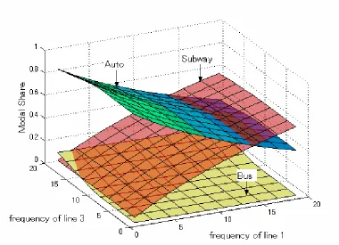
Fig. 5 shows the modal shares of the passengers between OD pair O1D1 when the
frequencies of transit lines of 1 and 3 vary, i.e. the subway line and bus line respectively,
where frequencies of line 2 and line 4 are fixed at 5 (services/hour). The modal share of
subway increases as the subway line frequency increases, i.e. changing from about 5% at a
subway frequency of 1 services/hour, to 50% at a subway frequency of 20 services/hour.
[INSERT FIGURE 5]
Similarly, the modal share of auto decreases as the subway line frequency increases,
changing from about 80% to 30%. As the subway line frequency changes, for O1D1 most
transport mode switching occurs between the subway and auto, with only a small change to
the bus’s share.
On the other hand, as the frequency of the bus line is increased, the modal share of
bus increases slightly and there is a small change to the share for auto and subway. The bus
network is heavily occupied by the passengers between OD pair O2D2, who can only use the
bus system. This is the reason for the insensitivity to the bus frequency of the bus share
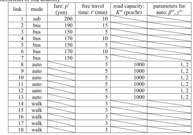
TABLE 1
Coefficients of link disutility
link mode fare: p s (yen)
free travel time: ts (min)
road capacity: Ksa (pcu/hr)
parameters for auto: sa, sa
1 sub 200 10
2 bus 190 15
3 bus 150 5
4 bus 170 10
5 bus 150 5
6 bus 170 10
7 bus 150 5
8 auto 5 1000 1, 2
9 auto 5 1000 1, 2
10 auto 5 1000 1, 2
11 auto 5 1000 1, 2
12 auto 5 1000 1, 2
13 auto 5 1000 1, 2
14 walk 3
15 walk 3
16 walk 3
17 walk 3
TABLE 2
Coefficients of line disutility
line mode
vehicle capacity ( l)
(passengers/service)
mode specific constants
( m)
coefficients for link disutility ( m, m, m)
parameters for waiting time function ( 2, 2)
parameters for discomfort
function ( 1, 1)
1 sub 100 10 1, 1, 0.02 2, 3 2, 3
2 bus 50 20 1, 1, 0.02 2, 3 2, 3
3 bus 50 20 1, 1, 0.02 2, 3 2, 3
4 bus 50 20 1, 1, 0.02 2, 3 2, 3
5 auto ∞ 50 1, 1, 0.02
In the case of the subway, the increase in the frequency of the subway service can
decrease the disutility of the subway system dramatically. Both the expected waiting time and
the in-vehicle discomfort decrease, so that passengers change transport mode from auto to
subway. Thus, the modal share of subway is relatively sensitive to the frequency changes of
the subway. This is different from the situation with the bus system.
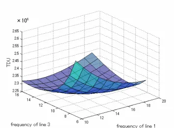
Next, we consider the FDP for the transit lines. Fig. 6 shows the surface of the
objective function as the frequencies of transit lines 1 and 3 vary (with fixed frequencies on
transit lines 2 and 4, of 5 services/hour). The fares per frequency increase (Fl) on transit line l
(=1,…,4) are set as 50, 20, 40 and 20, respectively. From Fig. 6, the objective function
suggested an optimal solution of the frequencies for transit lines 1 and 3 are not at the
boundary (i.e. interior solution).
[INSERT FIGURE 6]
With a lower level of frequencies for the transit lines, the expected waiting time and
in-vehicle discomfort increase, so does the total disutility in the network. In the case of a high
level of frequencies of the transit lines, both the expected waiting time and in-vehicle
discomfort decrease, while the disutility converted fare caused by frequency setting increases.
As a result, the total disutility in the multi-modal network increases as a whole. In general,
judging from these facts, an optimal solution of the FDP should be an interior solution (as
shown in Figure 6).
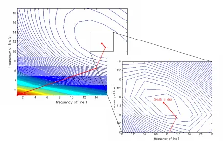
We applied the algorithm mentioned above to solve the optimal frequencies of the
transit lines problem. Fig. 7 shows the contours of the objective function (as shown in Fig. 6)
with the trajectory of the optimization process of f1 and f3 starting from a set of initial
solutions of ( f1, f3 ) = (1.00, 1.00). The optimal solution and the value of optimized objective
function found during the third outer iteration of the algorithm are (f1*,f3*)=(14.85 ,11.66)
and 2.2697×10⁶ respectively. The modal shares of subway, bus and auto by the passengers
respectively. The algorithm also obtained the same solutions even when we started the
optimization process from different initial solutions.
[INSERT FIGURE 7]
The solutions, obtained in the case when all frequencies of four transit lines are
optimized, are (f1*,f2*, f3*,f4*)= (12.57, 16.37, 1.00, 20.11), and the value of the objective
function at optimal frequencies is 2.2295×10⁶. The modal shares of subway, bus and auto by
the passengers between OD pair O1D1, at optimal frequencies of all lines, are 47%, 10% and
43%, respectively. Note that the optimal frequency of line 3 is calculated as 1.0, which is the
minimum value determined by the constraints. This implies that it is not worthwhile (against
the cost of improvement) to improve the frequency of line 3 to reduce the total disutility in the
multimodal network. In this context, it is better that line 3 is eliminated. The problem dealt
with here, i.e. FDP, can give one possible standard for judging transit’s efficiency in terms of
disutility that does not depend on profitability.
7.3. Results for the Anti-freezing Admixture Dispersion Problem
Fig. 8 shows changes in modal shares for the passengers between OD pair O1D1 both
in summer and in winter, based on the assumption that traffic capacities in winter decrease
from those in summer, where a vector of transit frequencies is set as f = (5, 10, 10, 10, ∞)T.
The calibration parameter in Eq.(46) is set equal to 1. From Fig. 8, there are large numbers
of passengers who change transport mode depending on the season, especially the change
from auto in summer to subway in winter.
[INSERT FIGURE 8]
Fig. 9 shows modal shares of the passengers between OD pair O1D1 when the amount
of AFMD on links 9 and 10 vary, while the amount of AFMD on the other links is fixed at 0.
Using AFMD on these two links brings about changes in transport mode between auto and
bus; on the other hand, the modal share of subway does not show any big differences.
Fig. 8. Modal shares of passengers between O1D1 in summer and winter seasons.
Subway Auto Bus *
Fig. 9. Modal shares of passengers between O1D1 for the AADP.
Fig. 10 shows the surface of the objective function as the amounts of AFMD on links
9 and 10 vary (with the amount of anti-freezing admixture dispersed on the other links fixed
at 0). The vector of deterioration costs per AFMD increase is set as Co8~13 = (800, 200, 800,
1000, 1000, 1000)T. From Fig. 10, the objective function seems to be more sensitive to the
amount of AFMD on link 9 than the amount on link 10.
[INSERT FIGURE 10]
Fig. 11 shows the contours of the objective function (as shown in Fig. 10) with the
trajectory of the optimization process of sal9 and sal10 starting from a set of initial solutions of
(sal9, sal10 ) = (0.00, 0.00). The optimal solution and the optimal value of the objective
function found during the third outer iteration of the algorithm are
) .06 2 , 97 . 3 ( ) ,
(sal9* sal10* = and 1.3852×10⁵ respectively. The modal shares of subway, bus
and auto by the passengers between OD pair O1D1, at optimal dispersions of link 9 and link
10, are 58.4%, 20.3% and 21.4%, respectively. The algorithm also obtained the same
solutions when we started the optimization process from different initial conditions. The
differences in the optimal amounts of AFMD on links 9 and 10 come from their deterioration
costs per AFMD increase. When the optimal dispersions are made in the winter season, the
ratios of capacities for links 9 and 10 correspond to 90% and 84% of those in summer season,
respectively.
[INSERT FIGURE 11]
The solutions, obtained in the case where amounts of dispersion on all road links are
optimized, are sal8~13 = (1.92, 5.06, 2.49, 0.53, 0.85, 0.53)T, and the value of the objective
function at optimal dispersions is 1.3540×10⁵. The amount of dispersion on link 8 is much
less than that on link 10 despite their same deterioration costs per a unit of AFMD, and
despite the fact that link 8 is used by all passengers between OD pair O1D1 who choose auto.
This is because of the different effects from bus lines, i.e. dispersion on link 8 cannot reduce
disutilities for the passengers who choose bus, whereas dispersion on link 10 can do this. The
season correspond to 82.8%, 91.7%, 85.7%, 67.3%, 73.0% and 67.3% of those in summer
season, respectively. The modal shares of subway, bus and auto by the passengers between
OD pair O1D1, at optimal dispersions, are 57.0%, 21.7% and 21.3%, respectively.
8. Concluding Remarks
In this study, a probit-based multi-modal transport assignment model is proposed.
Three transport modes⎯railway system, bus system and auto⎯are considered simultaneously
in the model, allowing for the interaction effect of the congestion caused by autos and buses.
Two network design problems, the FDP and AADP, are formulated as implicit programs in
which the objective functions are to minimize total disutility in the multi-modal network at
the SUE flows, by changing the network variables. Two numerical examples are given to
illustrate the model and algorithm proposed. It is found, based on some tests that the
algorithm finds the same optimal solution regardless of the initial conditions given. However,
the uniqueness of the solution may strongly depend on the coefficients of the disutility
functions, since these coefficients influence the uniqueness of the probit-based SUE flows for
a multi-modal traffic assignment with asymmetric link disutility functions. Further
examination of the uniqueness and stability of the multi-modal traffic assignment model
proposed in this study is required. This research topic will be addressed in a future study.
Acknowledgements
This research has been partially supported by the UK Engineering and Physical
Sciences Research Council grant GR/R53876/01. This research was partially carried out
during a one-year visit to Leeds by the first author. This visit was supported by the Japan
References
Abdulaal, M. & LeBlanc, L.J. (1979) Continuous equilibrium network design models, Transportation Research Part B 13 (1), 19-32.
Chiriqui, C. & Robillard, P. (1975) Common bus lines, Transportation Science 9, 115-21. Clark, S.D. & Watling, D.P. (2002) Sensitivity analysis of the probit-based stochastic user
equilibrium assignment model, Transportation Research Part B 36 (7), 617-35. Connors, R.D., Sumalee, A. & Watling, D.P. (2005) Sensitivity Analysis of the Variable
Demand Probit Stochastic User Equilibrium with Multiple User-Classes, Transportation Research Part B submitted.
De Cea, J. & Fernandez, E. (1993) Transit assignment for congested public transport system: An equilibrium model, Transportation Science 27, 133-47.
Fernandez, E., De Cea, J., Florian, M. & Cabrera, E. (1994) Network equilibrium models with combined modes, Transportation Science 28, 182-92.
Gao, Z.Y., Sun, H. & Shan, L.L. (2004) A continuous equilibrium network design model and algorithm for transit systems, Transportation Research Part B 38 (3), 235-50.
Kraus, M. (1991) Discomfort Externalities and Marginal Cost Transit Fares, Journal of Urban Economics 29, 249-59.
Kurauchi, F., Schomoecker, J.-D. & Bell, M.G.H. (2003) Capacity Constrained Transit Assignment with Common Lines, Journal of Mathematical Modelling and Algorithms 2, 309-27.
Lam, W.H.K., Gao, Z.Y., Chan, K.S. & Yang, H. (1999) A stochastic user equilibrium assignment model for congested transit networks, Transportation Research Part B 33 (5), 351-68.
Lawphongpanich, S. & Hearn, D.W. (2004) An MPEC Approach to Second-Best Toll Pricing, Mathematical Programming B 101 (1), 33-55.
Lo, H.K., Yip, C.W. & Wan, K.H. (2003) Modelling transfer and non-linear fare structure in multi-modal network, Transportation Research Part B 37 (2), 149-70.
Nielsen, O.A. (2000) A stochastic transit assignment model considering difference in passenger utility functions, Transportation Research Part B 34 (5), 377-402.
Shepherd, S.P. & Sumalee, A. (2004) A Genetic Algorithm Based Approach to Optimal Toll Level and Location Problems, Networks and Spatial Economics 4, 161-79.
Spiess, H. 1983, On optimal route choice strategies in transit networks, Pub. 286, Centre de Recherche sur les Transports, University of Montreal.
Spiess, H. & Florian, M. (1989) Optimal strategies: A new assignment model for transit network, Transportation Research Part B 23 (2), 83-102.
Sumalee, A., Connors, R. & Watling, D.P. (2005) Optimal toll design problem with improved behavioural equilibrium model: the case of Probit model. Mathematical and Computational Models for Congestion Charging, eds DW Hearn, S Lawphongpanich & MJ Smith, Springer, Berlin, Germany.
Tobin, R.L. & Friesz, T.L. (1988) Sensitivity Analysis for Equilibrium Network Flow, Transportation Science 22 (4), 242-50.