Advanced polarization control for optimizing ultrafast laser micro-processing

(1)

School of Engineering

PhD Thesis

Advanced polarization control for optimizing

ultrafast laser micro-processing

Thesis submitted in accordance with the requirements of the University of Liverpool for

the degree of Doctor in Philosophy

by

Olivier Allègre

(2)

(3)

(4)

Declaration

I hereby declare that all the work contained within this dissertation has not been submitted for any other qualification.

(5)

(6)

Summary

The ability to control and manipulate the state of polarization of a laser beam is becoming an increasingly desirable feature in a number of industrial laser micro-processing applications. Being able to control polarization would enable the improvement of the efficiency and quality of processes such as the drilling of holes for fuel-injection nozzles, the processing of silicon wafers or the machining of medical stent devices.

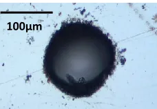
This thesis presents novel, liquid-crystal-based optical setups for controlling the polarization of ultrafast laser beams, and demonstrates how such optical setups can be used to improve laser micro-processing efficiency and quality. Two experimental strategies were followed: the first used dynamic control of the polarization direction of a linearly polarized beam; the second generated beams with complex polarization structures. Novel optical analysis methods were used to map the polarization structures in the focal region of these laser micro-processing setups, using Laser Induced Periodic Surface Structures (LIPSS) produced on stainless steel sample surfaces at low laser fluence (around 1.5J/cm²), close to the ablation threshold of steel (i.e. 0.16J/cm²). This helped to characterize and calibrate the optical setups used in this thesis.

The first experimental method used a fast-response, analogue, liquid-crystal polarization rotation device to dynamically control the direction of linear polarization of a laser beam during micro-processing. Thanks to its flexibility, the polarization rotator could be set-up in various synchronized configurations, for example keeping the polarization direction constantly perpendicular to the beam scanning motion. Drilling and cutting tests were performed on thin (~0.4mm thick) stainless steel sheets using a 775nm femtosecond laser at 24J/cm². The experimental results showed a consistent improvement in the micro-processing quality when the polarization direction was synchronized with the beam scanning motion. The sidewall surface roughness and edge quality of the machined structures were improved significantly, with the dimensions of ripples and distortions divided by a factor of two. The overall processing efficiency was also increased compared to that produced by linear or circular polarizations.

(7)

experimental results and clarified how the polarization and phase structures affect the focal properties of the produced laser beams.

(8)

List of publications to date by author

Allegre O. J., Perrie W., Edwardson S. P., Dearden G., Watkins K. G., 2012, Laser microprocessing of steel

with radially and azimuthally polarized femtosecond vortex pulses, J. Optics 14 (8): 085601

Allegre O. J., Perrie W., Bauchert K., Liu D., Edwardson S. P., Dearden G., Watkins K. G., 2012, Real-time control of polarisation in ultra-short-pulse laser micro-machining, Appl. Phys. A 107 (2): 445-454

Allegre O. J., Perrie W., Edwardson S. P., Dearden G., Watkins K. G., 2011, Ultra-short pulse laser

micro-machining of metals with radial and azimuthal polarization, Proc. ICALEO 2011: 917-925

Allegre O. J., Perrie W., Bauchert K., Dearden G., Watkins K. G., 2010, Real-time control of polarisation in

high-aspect-ratio ultra-short-pulse laser micro-machining, Proc. ICALEO 2010: 1426-1433

Allegre O. J., Perrie W., Bauchert K., Liu D., Edwardson S. P., Dearden G., Watkins K. G., 2010, Real-time

control of polarization in ultra-short pulse laser micro-processing, Proc. MATADOR 2010: 553-556

Croft J., Edwardson S. P., Williams C. J., Allegre O. J., Dearden G., Watkins K. G., 2010, Embedding arrays

(9)

(10)

Acknowledgements

I would like to thank Ken Watkins (my primary supervisor), Geoff Dearden, Stuart Edwardson and Walter Perrie, who have an inexhaustible supply of scientific insight and enthusiasm, which has meant that my Ph.D. has been not only interesting, but also enjoyable.

It is impossible to spend four years at the Laser Group without appreciating Doug Eckford, who has persistently made sure that the computers are running smoothly, as well as Eamonn Fearon who has tirelessly ensured the smooth running of the Lairdside Laser Engineering Centre, where most of the experimental work has been done. It has been lovely to meet and work alongside so many members of the Laser Group.

(11)

(12)

1

Introduction

1.1 Background to laser technology

The laser is undoubtedly the most important optical technology to be developed in the past 60 years. Soon after Theodore Maiman demonstrated the first ruby laser in 1960, there were tremendous developments in the field of laser technology. As a result, a wide range of basic laser applications quickly appeared in various domains such as surgery, bar-code scanning, telecommunication and industrial manufacturing (S. Perkowitz, 2010). The latter is the focus of this thesis.

1.1.1 Principle of the laser

A laser is a device that emits coherent electromagnetic radiation in the infrared, visible or ultraviolet spectrum, through a process of optical amplification based on the stimulated emission of photons. A laser is constructed from three principal elements: an energy source, a gain medium and an optical cavity (Figure 1.1).

 The energy source (also referred to as pump source) provides energy to the laser system. The energy source can be for example an electrical discharge, or the light from a flash lamp or another laser.

 The gain medium is a material (either a gas, liquid or solid) with optical properties that determines the characteristics of the laser light, such as its wavelength. Each electron in the gain medium carries some energy. Quantum mechanical effects dictate that electrons can only carry discreet energy levels. At a given time, an electron carries a defined level of energy, within the set of energy levels allowed by the material. In a laser gain medium, the electrons can be either in a ground state (they carry a minimum level of energy), or in an excited state (they carry a higher level of energy). The difference between the energy levels of the ground and excited states determines the wavelength of a laser. Typically, a laser gain medium does not have one, but multiple excited states (i.e. a multitude of allowed energy levels).

 The optical cavity (also referred to as optical resonator) is a set of mirrors placed around the gain medium so that photons can travel back and forth through it. Typically in a simple two-mirrors optical cavity, one of the mirrors is highly reflective and the other is partially reflective to allow some of the light to leave the cavity. It is noted that optical cavities can also use a more complex configuration, for example a ring cavity.

(19)

where the electrons in an excited states transfer their energy to incoming photons, producing more photons as a result (these electron-photon energy transfers are also called lasing transitions). The photons are reflected by the mirrors of the optical cavity, so that they travel back into the gain medium where they produce more stimulated emission. The photons may reflect back and forth inside the cavity many hundred times before exiting the cavity, through a partially reflective cavity mirror for example.

Although in principle lasers produce monochromatic light (electromagnetic radiation of a single wavelength), most lasers actually produce radiation in several modes, each having a slightly different frequency (wavelength). Some lasers even produce radiation in a wide spectral range, as much as 20nm in some cases. Lasers can operate in continuous mode, where the output beam power is constant over time. Such lasers are known as continuous wave lasers (CW lasers). Lasers can also operate in pulsed mode.

(20)

1.1.2 Industrial laser manufacturing

Right from the outset, the potential usefulness of laser-material interactions in industrial manufacturing applications was envisaged. Industrial laser manufacturing generally involves focusing a laser beam to melt or ablate material in a work-piece. Theoretical and experimental studies were soon undertaken to better understand these interactions. For industrial manufacturing processes such as cutting, welding and surface treatment, the quality of the laser source is of primary importance. In particular, achieving a good process efficiency requires the use of laser sources that produce a high average-power.

1.1.2.1 High-average-power laser sources for industry

Two early laser technologies demonstrated such high-average-power: CO₂ laser sources (which were first demonstrated by C. K. N. Patel, 1964) and Nd:YAG laser sources (first demonstrated by J. E. Geusic

et al. 1964). Both technologies can produce continuous or pulsed output beams and work in the infrared

spectrum (10.6μm for the CO₂ laser and 1.06μm for the Nd:YAG laser). CO₂ laser sources started being adopted in industry in the late 1960s, followed by the Nd:YAG laser sources in the 1970s.

Another technology, the Excimer laser (first demonstrated by N. Basov et al. 1970), produces a high-average-power, pulsed output beam in the ultraviolet spectrum. Excimer laser sources started being adopted for semiconductor wafer processing applications in the microelectronics industry from the early 1980s. In particular, the Excimer laser lithography technique, which was first demonstrated by K. Jain et al. (1982), is now arguably the only widely used technology for the manufacturing of microelectronic devices.

An additional technology, the laser diode, was initially demonstrated by both R. N. Hall et al. (1962) and M. I. Nathan et al. (1962). The laser diode started being used in telecommunication and information technologies from the 1980s. Since 1990, technology improvements enabled diode lasers to produce high-average-power beams. This led to their use for solid-state laser cavity pumping and enabled the advent of Diode-Pumped Solid-State (DPSS) lasers (J. Hecht, 2010). This also led to the use of laser diodes as direct sources for industrial processing applications such as surface hardening and welding, with diode arrays generating as much as 100W in average power, in continuous mode (first demonstrated by M. Sakamoto et al. 1992).

1.1.2.2 Emergence of integrated industrial laser processing systems

Apart from a high-average-power laser source, high-quality industrial laser processing also requires advanced beam quality control, in-process optimization of the output power and beam delivery, etc... All these areas saw rapid technological developments in the 1960s and 1970s (W. M. Steen, 1991; R. Crafer & P. J. Oakley, 1993).

(21)

1.1.2.3 Emergence of high-precision industrial laser micro-processing

Another area of development for industrial laser manufacturing is in high-precision micro-applications (for example in the microelectronics, photonics or medical industries), where ever more accurate processes are required. This fueled the development of short-pulse lasers, with pulse lengths in the nanosecond range. By concentrating the available energy into short time intervals, these short-pulse lasers provide a higher peak-power and enable a more accurate control of laser-material interactions. This, in turn, increases the machining quality by reducing recast and molten material during processing (D. Breitling et al. 2004a). A variety of such nanosecond-pulse laser sources have been developed since the 1980s. These include for example the Q-switched Nd: YAG lasers, the ytterbium-doped fiber lasers (J. Hecht, 2010), or the thin-disk lasers (first demonstrated by J. A. Abate et al. 1981).

(22)

1.2 Introduction to ultrafast laser micro-processing

A laser source that produces light pulses with a duration in the picoseconds ( s) or femtosecond ( s) range is referred to as an ultrafast, or ultrashort-pulse laser. Shortly after their invention (P. F. Moulton, 1986), ultrafast lasers were mostly used for ultrafast spectroscopic applications, where their incredibly short pulse length facilitated the study of how the energy states and electron dynamics of molecules affect complex chemical or biological processes (A. Cavalieri, 2010). However it quickly emerged that their high peak power and very short laser-material interaction duration could also be beneficial to micro-manufacturing applications.

Producing such pulse durations at the level of pulse energy required for micro-manufacturing processes is generally achieved with a combination of advanced optical techniques, such as mode locking and chirped pulse amplification. Mode locking enables the production of extremely short, low energy (nJ) laser pulses, whereas chirped pulse amplification enables their amplification to achieve a pulse energy in the millijoule range, as required in micro-manufacturing applications. Most of the experimental work described in this thesis uses a femtosecond-pulse laser source, namely a Clark-MXR CPA2010 Ti-Sapphire laser. This laser source has a titanium-doped sapphire gain medium and uses mode locking and chirped pulse amplification to produce a femtosecond pulse train at a wavelength of 775nm.

1.2.1 Mode locking

1.2.1.1 Principle

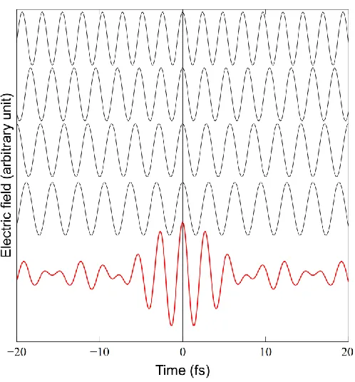
Mode locking is a technique which is used to produce ultrashort laser pulses by inducing a fixed phase relationship between the oscillating electromagnetic field modes (i.e. the longitudinal modes) of the laser’s optical cavity. By their nature, ultrashort-pulse lasers emit radiation over a broad range of wavelengths. For example a 180fs-pulse laser can have a wavelength range of 5nm around a central wavelength of 775nm (Z. Kuang et al. 2009a). Thanks to mode locking, the wavelength components are timed exactly so that their electromagnetic field modes nearly cancel each other out, except for during one tiny period of time when they combine constructively in one intense pulse (see Figure 1.2).

The wavelength of electromagnetic radiation modes that oscillate in a laser’s optical cavity are determined by two factors. The first one is the lasing transitions that occur in the laser gain medium. In an ultrashort-pulse laser, the gain medium is chosen to have a broad range of lasing transitions (i.e. a large gain bandwidth ∆ν). For example, a titanium-doped sapphire has a lasing wavelength range of approximately 300nm centered near 800nm i.e. a gain bandwidth ∆ν of 130THz, and hence can support a temporal pulse-length τ 1/∆ν 8fs (A. Cavalieri, 2010). The second factor is the length of the optical cavity that surrounds the gain medium. The cavity length allows a set of discrete wavelength components (i.e. those that have an electromagnetic field mode with nodes at the cavity’s end mirrors) to be amplified. By mode locking a broad range of wavelengths, an ultrashort pulse is produced at a dynamic point in the cavity, at which the many electromagnetic field modes interfere constructively. This point of coincidence moves back and forth in the cavity at the speed of light.

1.2.1.2 Methods to achieve mode locking

(23)

other modes and the resulting output beam power would fluctuate randomly. To achieve mode locking, two sets of methods have been developed, referred to as active and passive mode locking.

 Active mode locking uses a dynamic light modulation device in the laser cavity, externally driven with a synchronized signal. This is usually an acousto-optic modulator, which acts as a controllable attenuator. The light bouncing between the mirrors of the cavity is either attenuated when the device is “off”, or transmitted through when it is “on”. The modulator is “switched on” periodically each time the pulse has completed a cavity round trip.

 Passive mode locking uses a saturable absorber inside the cavity. A saturable absorber attenuates low-intensity light and transmits high intensity pulses.

Both active or passive, mode locking allows selective amplification of a high-intensity pulse travelling round trips between the cavity mirrors. As a result, a mode locked laser cavity produces a train of ultrashort pulses.

It is noted here that lasers which operate in a continuous wave fashion (CW laser) have their electromagnetic radiation modes oscillating randomly in the laser cavity, with no fixed relationship between each other. This leads to a near-constant output intensity with no laser pulses. Unlike pulsed lasers, continuous wave lasers generally emit radiation with a single monochromatic frequency.

[image:23.612.192.441.373.641.2]

(24)

1.2.2 Chirped pulse amplification

For ultrafast laser material processing applications, ultrashort pulses need to be amplified in energy to the millijoule level. Amplifying an ultrashort laser pulse to these energy levels directly would damage the amplification crystal (gain medium), because of the very high peak power contained in the pulse. A chirped pulse amplification technique is used to avoid this.

In a chirped pulse amplifier, a seed ultrashort laser pulse is stretched in time to as long as a nanosecond by inducing a relative delay between its wavelength components (i.e. its longitudinal modes) to reduce peak intensity, prior to introducing it to the gain medium. This is usually achieved using a pair of gratings that are arranged so that the longer wavelength components of the laser pulse travel a shorter path than the shorter wavelength components. After the gratings, the shorter wavelength components lag behind the longer wavelength components (see Figure 1.3). The stretched pulse, which has a lower peak intensity, is then safely introduced to the gain medium for amplification. Depending on the design of the laser, the pulse can travel several times within the cavity, to deplete the amplification crystal (i.e. the gain medium) of its stored energy, before being released out of the laser cavity. Following amplification, the pulses are recompressed by temporally reversing the stretching process and removing the relative delay between the wavelength components. In this way, ultrashort laser output pulses achieve much higher peak powers, as the amplification is not limited by the damage threshold of the amplifying crystal.

(25)

1.2.3 Laser-material interactions mechanisms

This section gives a brief overview into various types of laser-material interaction mechanisms which occur when a pulsed laser beam is used to process a material. A distinction is made between two types of processing regimes. The first is when a laser beam with a “long” pulse duration (i.e. down to the nanosecond range) is used. This is typically referred to as the long-pulse regime. The second is when a pulse duration in the picosecond or femtosecond range is used. This is sometimes referred to as the ultrashort-pulse regime. Each of these regimes produces different types of laser-material interactions.

1.2.3.1 Long-pulse regime

Micro-machining materials such as metals or semiconductors in the long-pulse regime is a dynamic process where the material close to the surface of the work-piece is heated, molten and finally vaporized within the duration of each pulse (S. T. Hendow & S. A. Shakir, 2010). In this regime, laser pulses transfer most of their energy thermally by melting the material. However, energy losses occur due to thermal diffusion within the pulse duration. Thermal diffusion causes heat to flow to the bulk substrate material outside the processing area and reduces the efficiency of the process.

To improve efficiency, high-precision industrial processes often use pulse lengths in the nanosecond range, since they produce less thermal losses than longer pulses in the microsecond range or above. This results in a comparatively high processing speed. However even with nanosecond pulses, melting inevitably produces recast layers on the sidewalls of the machined structures, which limits the end quality of the process achievable in this regime (N. H. Rizvi, 2003).

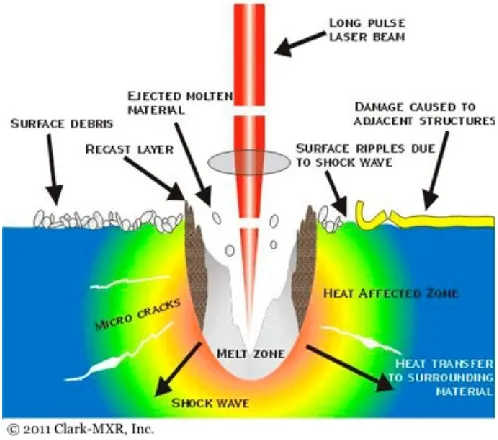
For any given micro-machining process, a balance has to be found between efficiency and quality. For example by increasing the pulse energy, more material is ablated by each pulse, making the process more efficient; however, this also produces more recast material on the sidewalls of the machined structures (Figure 1.4) and this reduces the process quality.

[image:25.612.182.431.448.668.2]

(26)

1.2.3.2 Ultrashort-pulse regime

In the ultrashort-pulse regime, the heat deposited by the laser into the material does not have enough time to move away from the processing area within the duration of the pulse. This reduces thermal diffusion and energy losses. As soon as a laser pulse reaches the surface, the temperature at the focal spot rises very quickly past the melting point and then the evaporation point of the material, soon reaching the plasma regime (C. Fohl & F. Dausinger, 2006; D. Breitling et al. 2004b). As a result, ultrashort-pulses increase the share of vaporized material at the expense of molten material. They enable many materials to be processed with a very high quality and minimal thermal damage (see Figure 1.5).

The physics of laser material interactions in this regime can be described as follows: when an ultrashort pulse reaches the target surface, the laser radiation energy is absorbed locally in the electron system of the target material. Depending on the fluence and peak power of the laser pulse and on the properties of the target material, various laser-material energy transfer mechanisms can occur:

 In some semiconductors or dielectric materials, the intense energy transfer to the electrons causes their separation from the bulk material, leaving behind ions which repel each other and leave the bulk substrate material. This process is referred to as a Coulomb explosion (F. Dausinger, 2003).

 Another example of an energy transfer mechanism is multi-photon absorption, which occurs in some dielectrics. Here, the high peak power of the ultrashort pulses causes the laser photons to excite molecules within the target material to their higher energy state.

 In metals, each laser pulse locally heats electrons. Contrary to the light-weight electrons, the heavier ion lattice of the material cannot absorb optical radiation energy directly since they cannot follow the fast oscillations of the electromagnetic field. However, by collisions with the energetic electrons, the ion lattice is also heated up eventually. Due to the large mass difference between electrons and ions, only a small energy portion can be transmitted by each electron-ion collision (D. Breitling et al.

2004a). Thermodynamic equilibrium between the electron system and the lattice is only reached after a time delay in the nanosecond range, after which the transferred energy vaporizes the material. Since the duration of the laser pulse is shorter than this time delay, it does not transfer its energy to the lattice directly. This reduces melt formation and thermally induced stress and it leads to a better process quality.

(27)

(28)

1.2.4 Techniques for laser micro-machining

Laser micro-machining (also referred to as laser micro-processing) is a general term that includes a variety of processes, such as surface marking, hole drilling, cutting and milling. This section gives a brief overview of some of the processes used to micro-machine metals with short- and ultrashort-pulse lasers.

1.2.4.1 Low aspect-ratio processing

Low-aspect-ratio processing includes the marking or texturing of the surface of a work-piece, as well as drilling or cutting structures through thin sheets of material (thin semiconductor wafers, metal sheets etc…). It involves the gentle surface ablation of target materials. Ultrashort pulses with a fluence just above the ablation threshold can be used to produce virtually melt-free structures (D. Breitling et al.

2004a). The low processing efficiency associated with low pulse energy can be compensated by increasing the pulse repetition rate of the laser source. The laser is scanned across the surface to produce the desired geometry. The number of pulses at each position determines the depth of the structures.

1.2.4.2 High-aspect-ratio micro-drilling

For high-aspect-ratio laser drilling, a high enough fluence is necessary to maintain a good ablation efficiency. Experimental evidence shows that deep hole drilling generally requires a high fluence level to enable full material penetration (D. Breitling et al. 2004b). Therefore thermal damages such as the formation of melt and heat affected zones, which occur during high-fluence laser processing, can be problematic even with ultrashort pulses (F. Dausinger, 2003; D. Breitling et al. 2004b). Specific machining techniques have been developed to limit these effects.

There are four principal techniques for laser drilling: single-pulse, percussion, trepanning and helical drilling (see Figure 1.6). Single-pulse and percussion are simpler and faster drilling methods since they use only the focused laser beam for machining, without any further optics. The resulting hole is roughly the same diameter as the laser beam’s spot size. These methods can deliver aspect ratios as large as 10; however, they do not produce the best hole quality. Trepanning and helical drilling are more complex as they involve moving the laser beam with regard to the work-piece. As a result these methods produce holes wider than the laser beam spot size.

Laser trepanning involves piercing the work-piece in the same way as in percussion drilling and then cutting a round hole in one circular movement. Laser trepanning is comparable to a cutting process. Again, this method can suffer from melt formation and heat affected zones.

(29)

with a very high aspect-ratio (i.e. above 10). The hole quality can also be further improved by using an assist gas during drilling to reduce oxidation, or by drilling at reduced atmospheric pressure to facilitate ablation and molten material ejection. It is noted that in some cases helical drilling can be used to produce non-circular holes. Instead of repeatedly scanning along a circular path, the laser beam can follow a specific path to produce the desired hole geometry.

1.2.4.3 Micro-milling and cutting

For machining more general shapes which are not necessarily circular or do not go through the full thickness of the work-piece, various methods can be used, such as milling or cutting. For example micro-machining non-circular holes through the work-piece can be achieved by cutting out, removing a core in the centre of the scanned beam path. As in helical drilling, the beam scans repeatedly over the work-piece. However unlike in helical drilling, there is a core left which is removed after machining.

In some cases, blind structures are desired, which do not go all the way through the thickness of the work-piece. As before, the laser is scanned across the surface to produce the desired structures (N. H. Rizvi, 2003). The number of pulses at each position determines the depth of the structure. This process is often referred to as micro-milling.

1.2.4.4 Further developments in current micro-machining techniques

In all laser micro-machining applications, the quality of the produced features has to be balanced with the process efficiency and cost. Thus, current industrial applications require a careful adjustment of process parameters such as the fluence, pulse duration, wavelength or pulse repetition rate of the incident laser beam (S. Hahne et al.2007).

(30)

(31)

1.3 Introduction to phase and polarization

In this thesis, novel methods are used to control the phase and polarization of laser beams. This section gives an overview into the physical meaning of phase and polarization and describes how these physical quantities can be described mathematically.

1.3.1 Definition of phase and polarization

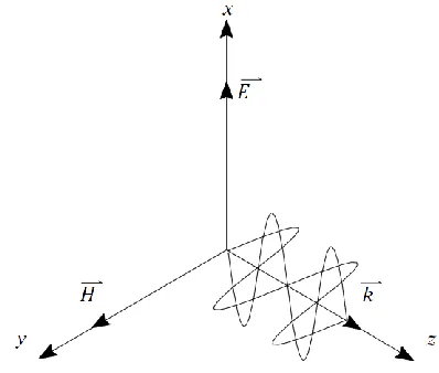
An electromagnetic wave produced by laser radiation can be described as a self-propagating, transverse oscillating wave of electric and magnetic fields. The electric and magnetic fields both oscillate perpendicularly to the direction of wave propagation and perpendicularly to each other. Each of these fields can be described as a sinusoidal function, oscillating in both space and time (see Figure 1.7).

1.3.1.1 Phase

If we plot the electric field along the axis of propagation of the laser beam at a given time, there are places along the axis where the field is at a maximum amplitude (i.e. a maximum positive field), places where it is zero and other places where the field is at a minimum amplitude (i.e. a maximum negative field), forming a sinusoidal function overall (Figure 1.8-a). These places along the axis of propagation represent different phases of the wave (D. C. O’Shea, 1985). In other words, the phase of an electromagnetic wave can be defined as the location where the sinusoidal function has a given amplitude value (see Figure 1.8-b). The concept of phase is valuable in the context where a group of coherent electromagnetic waves travel together in the same direction, as is the case in a laser beam. In such cases, it can be useful to describe a phase front (also referred to as wavefront) as a surface defined by the locations in space where all the sinusoidal functions have the same amplitude. In an undisturbed collimated laser beam, the phase front is generally a planar surface. In a focused laser beam, for example, the phase front has a convex shape (Figure 1.9).

1.3.1.2 Polarization

The polarization of electromagnetic waves is a property related to the orientation in which they oscillate. By definition, it is described by specifying the orientation of the wave’s electric field at a point in space, over one period of oscillation of the wave (D. C. O’Shea, 1985). For example, an ultrafast laser source typically produces a beam where the field is oriented in a single direction (i.e. it always oscillates along a fixed line in space; see D. Breitling et al. 2004b). This is referred to as linear polarization. However other types of laser sources can produce a field that rotates as the wave travels, producing polarization configurations called either circular or elliptical depending on the way the field rotates. It is noted that some laser sources produce beams where the direction of the electric field changes randomly over time. These beams are said to be randomly polarized. Laser sources that generate random polarization typically cannot produce ultrashort pulses for material processing (D. Breitling et al.

2004b), therefore random polarization is not investigated further in this thesis.

(32)

Figure 1.7: Schematic showing an electromagnetic wave represented in a coordinate system ( ) and propagating along the axis. An electromagnetic wave can be pictured as a combination of electric ( ) and magnetic ( ) fields whose directions are perpendicular to the direction of propagation of the wave ( ). This schematic is taken from D. C. O’Shea (1985).

Figure 1.8: (a) Schematic showing how the amplitude of the electric field E of an electromagnetic wave oscillates along the direction of propagation z. (b) Schematic showing phases of the wave. The solid lines indicate the places where the field is at a maximum +A, the dashed lines indicate the places where it is at a minimum –A. Each of these places represents a phase of the wave.

Figure 1.9: Schematic showing the planar wavefronts of a collimated laser beam (left), converging after a focusing lens (right).

a)

[image:32.612.204.403.72.241.2]

(33)

1.3.2 Mathematical representation of polarized light: Jones vectors

This section gives a brief reminder of Jones formalism, which uses complex vectors to describe polarization. For a more detailed description of Jones formalism, see for example F. L. Pedrotti & L. S. Pedrotti (1993) or J. P. Perez (1996). For a description of complex numbers, see for example K. F. Riley et al. (2002). It is noted here that I use the notation as an imaginary (i.e. complex) number and the notation as a Jones vector.

1.3.2.1 Reference coordinate system

To explain Jones vectors, we consider a ray of linearly polarized light, with its direction of propagation oriented perpendicularly out of this page and situated at the origin of the reference coordinate system defined in Figure 1.10. The electric field of the light is represented by a vector in this coordinate system. Here, it is chosen to be at +45˚ of the coordinate axes ( and ). The field oscillates periodically like a sinusoidal function along the direction indicated by the dotted line (see Figure 1.10). For convenience the vector is represented with the amplitude when the field is at its (positive) maximum. The vector is described in the coordinate system by the sum of its projections on the and axes of the coordinate system:

(1.1)

_and _{are unit vectors along the} _and_{axes of the coordinate system.} _and _{are often referred}

to as the components of the electric field vector.

Here, the Jones vector representing the polarization of the light is noted and is defined as: .

Each component and of the Jones vector is expressed as complex numbers: and

_{, where} _and _{, are the amplitude and phase of} _{respectively, and similarly for} _. The state of polarization is completely determined by the relative amplitudes and phases of these components. Therefore, Jones vectors are convenient to mathematically describe polarized laser beams. It is noted that the electric field vector is fully defined by the corresponding Jones vector . Henceforth in this thesis, I refer to Jones vectors using either the notation or , for clarity, depending on the circumstances.

In this example, the electric field vector is oriented at +45˚ of the axes of the coordinate system. Therefore the amplitudes and are equal.

Figure 1.10: Schematic showing the vector of a linearly polarized ray of light directed perpendicularly to the plane of this page, represented in a coordinate system .

(34)

1.3.2.2 Jones vector for linearly polarized light

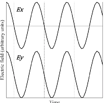
With a linearly polarized light (see Figure 1.10), both phase components and are equal (for convenience, they are both set equal to zero). In this case, both electric field components and are in phase and oscillate together, reaching their maximum amplitude at the same time, decreasing and reaching their minimum amplitude at the same time and so on (see Figure 1.11). Therefore, the resulting vector oscillates only within one orientation (i.e. along the dotted line in Figure 1.10). If we define for example , the Jones vector representing linear polarization is: .

1.3.2.3 Jones vector for elliptically polarized light

If the two phase components and are not equal, the electric field components and are not in phase and do not oscillate together. For example when reaches a maximum, is still increasing. When reaches its maximum has already started decreasing and so on (see Figure 1.12). This, in general causes the electric field vector to change its orientation and amplitude over time. As the field vector forms an elliptical pattern over a period of oscillation, this type of polarization configuration is called elliptical. This is generally described by defining and . If we define for example , we have the following Jones vector: , which defines in general an elliptical polarization.

1.3.2.4 Jones vector for circularly polarized light

(35)

Figure 1.11: Plot showing the time dependence of thecomponents and of an electric field vector representing a linearly polarized ray of light. Here, = , .

[image:35.612.224.400.61.236.2]

Figure 1.12: Plot showing the time dependence of thecomponents and of an electric field vector representing a elliptically polarized ray of light. Here, , , .

(36)

1.3.3 Mathematical representation of waveplates: Jones matrixes

In this section we explain, using matrices, how birefringent optical components such as waveplates affect the polarization of light transmitted through them. For a detailed description of matrix mathematics, see K. F. Riley et al. (2002).

1.3.3.1 Waveplates and Jones matrixes

A waveplate, or phase retarder, is an optical element that introduces a phase difference between the electric field components and (A. Yariv & P. Yeh, 1984). It works by making each component of the electromagnetic wave (corresponding to the electric field or ) travel through it with a different speed. As a result, there is a cumulative phase difference between the two wave components as they emerge from the waveplate. The phase difference is the main attribute of a waveplate. The physical phenomenon that causes each component of the electromagnetic wave to travel at different speeds is called birefringence and will be further detailed in Section 1.3.4.

Here we are interested in mathematically describing waveplates by using matrixes. A matrix that represents a waveplate is called a Jones matrix, and can be defined as:

(1.2) We describe the polarization of the electromagnetic wave incident on a waveplate using a Jones vector noted . The polarization of the wave that emerges from this waveplate is noted . By definition, the relation between the Jones vectors and is as follows:

(1.3)

1.3.3.2 Case where linearly polarized light is incident on a waveplate

If is the linearly polarized light described in Section 1.3.2.2 above, we have . Then we can derive in the following way:

(1.4)

Equation (1.4) is the mathematical expression that the waveplate introduces a phase difference between the electric field components and of the incident wave.

For example if the linearly polarized light described in Section 1.3.2.2 above, , is incident on a

waveplate with a value of , the resulting Jones vector is . In other words, the waveplate

has introduced a phase shift of (i.e. a quarter of periodic oscillation) between the components of the electric field. As a result, the incident linear polarization has been converted to circular polarization, defined by the Jones vector , as the field emerges from the waveplate. This type of waveplate is called quarter-waveplate, as it induce a phase retardance of a quarter of the period of oscillation of the electric field (i.e. a phase of ).

1.3.3.3 Case where circularly polarized light is incident on a waveplate

If the incident light, , is the circularly polarized light described in Section 1.3.2.4 above, we have

(37)

(1.5) Here, the waveplate introduces an extra phase shift between the electric field components and

of the incident wave. As the incident polarization was circular (i.e. with an existing phase shift of

between and ), the resulting overall phase shift after emerging from the waveplate will be .

If the waveplate has a phase retardance value of (i.e. a quarter-waveplate), the overall phase

shift of the resulting wave will be . Therefore the resulting Jones vector will be . In

complex number formalism, . Thus we have , which defines a linear polarization, with a direction of electric field oscillation oriented orthogonally to that of the incident light. Here, we have shown that a circularly polarized beam incident on a quarter-waveplate is converted into a linearly polarize beam.

In this thesis, various phase retardance optics are used to introduce a phase shift between the two electric field components of a laser beam and convert its polarization state.

1.3.4 Birefringence

Certain materials have anisotropic optical properties. For example, birefringent materials are so named because they have two distinct values for refractive index. This is due to the anisotropic forces binding the electrons of these materials, causing anisotropic response to a stimulating electromagnetic wave propagating through them. In other words, the electrons tend to oscillate preferentially along one direction, where the binding force is weaker (see F. L. Pedrotti & L. S. Pedrotti, 1993).

We can define a reference coordinate system with and axes directed perpendicularly to the light propagation, so that the axis corresponds to the direction of the strong binding force, where the electron oscillation is weaker (also called the optical axis of the material) and is perpendicular to (i.e. along the preferential direction of electron oscillation). The presence of anisotropic binding forces along the and directions leads to different refractive indexes: corresponding to the component of electric field oscillation along the axis and corresponding to that along the axis. This results in different velocities of light propagation along each axis: light travel faster along the axis, where the interaction with the electrons of the material is weaker (the axis is sometimes referred to as the fast axis).

This type of optical behavior occurs in materials such as calcite crystal, which have an anisotropic crystalline structure. It is noted that birefringence is also dependant on wavelength and that a given material is only birefringent within a portion of the electromagnetic spectrum. Birefringence is used to make phase retardance optics, such as waveplates. This is done by cutting and polishing a birefringent material in a direction parallel to its optical axis.

1.3.5 Fresnel’s coefficients and Brewster’s angle

(38)

To describe this, we can consider the case where a narrow beam of polarized light is incident at an arbitrary angle on a flat surface, as represented in Figure 1.14. A distinction is made between light which is polarized parallel to the plane of incidence (i.e. with the electric field oscillating within the plane of the page, see Figure 1.14) and light which is polarized orthogonal to the plane of incidence (i.e. with the electric field oscillating in a direction perpendicular to the plane of the page). The former is often referred to as p-polarization, or and the latter as s-polarization, or . The incident light can consists of a combination of a p-polarized component an s-polarized one.

The reflectivity of a material illuminated under p-polarized light is not always the same as that of the same material under s-polarized light. These reflectivities can be calculated using the well-known Fresnel formula (S. Nolte et al. 1999; F. Dausinger & J. Shen, 1993):

(1.6)

(1.7) and are the amplitude ratios of the reflected to incident electric fields for p- and s-polarized light respectively, with and as the electric field amplitude of the incident and reflected light respectively. is the angle between the direction of the incident light and the surface normal. The reflectivity for both p- and s-polarized light is then obtained from:

(1.8)

(39)

Figure 1.14: Schematic showing a beam of light (top left) incident on the surface of a material. The incident beam consists of both a p-polarized component and an s-polarized one. Some of the incident power is absorbed by the material and some is reflected from the surface. Depending on the angle of incidence , the value of reflectivity is not always identical for the p-polarized component and for the s-polarized one.

Figure 1.15: Reflectivity of steel as a function of the angle of incidence , for p- and s-polarized light illumination. Various types of steel have slightly different value of reflectivity. This plot is taken from S. Nolte et al. 1999.

(40)

1.3.6 Cylindrical Vector Beams

Most past research in industrial laser processing dealt with spatially uniform states of polarization, such as linear, elliptical and circular polarizations. In each of these cases, the state of polarization does not depend on the spatial location within the profile of the laser beam: the state of polarization is the same at all locations within a given beam cross-section. Recently, there has been an increasing interest in laser beams with a spatially varying state of polarization (Q. Zhan, 2009). Spatially structuring the state of polarization of a laser beam affects its focal properties, when focused by a lens, as well as the way it interacts with materials.

Of particular interest is the case where the oscillating electric field vectors are cylindrically symmetric around the cross-section of the laser beam. Such beams are often referred to as Cylindrical Vector Beams (CVBs). Two particular cases of CVBs are those with a radial or an azimuthal polarization structure (Figure 1.16). For example, the Jones vector representing an azimuthally polarized laser beam can be written as:

(1.10)

represents the polar angle in a Cartesian coordinate system (see Figure 1.16-c). In this configuration, the Jones vector (which varies spatially with the polar angle ) represents an electric field always oscillating in an azimuthal orientation, regardless of . It is noted that this Jones vector should not be confused with that representing a linear polarization oriented at an angle . The latter does not vary spatially with the polar angle .

In the example describe in Equation 1.10 above, the CVB only has a polarization structure (azimuthal in that case). It does not have a phase structure (i.e. the beam has a planar wavefront). CVBs can also be produced with a spatially varying phase structure such as a vortex phase. A beam with a vortex phase structure can be described as if it had a helical phase front, or a topological charge in its phase structure. This is why these types of beams are said to carry an Orbital Angular Momentum (OAM). Laser beams can have both a polarization and a phase structure (M. Beresna et al.2011). For example, the Jones vector representing an azimuthally polarized vortex phase beams can be written as:

(1.11)

The second term in Equation 1.11 represents an electric field oscillating azimuthally as detailed in Equation 1.10 above. The first term is the phase vortex element. For example the electric field oscillating at a polar angle in the coordinate system has a Jones vector , whereas

the electric field oscillating at an angle has a Jones vector . This means

has a phase delay of compared to . The overall phase structure of the beam forms a vortex pattern (Q. Zhan, 2009).

The transformative properties of CVBs such as those with a radial or azimuthal polarization and/or a vortex phase structure include their isotropic laser-material interactions, controllable laser-material energy coupling, and sub-diffraction limited focal spot size. Moreover, they also enable a greater control over the focal energy distribution (Q. Zhan, 2009). Some of these structured beams are starting to be explored for microscopy and telecommunication applications. The field of laser manufacturing is another very promising and yet not very well explored application.

(41)

planar phase and radially and azimuthally polarized beam with a pitch phase vortex (i.e. a topological charge of 1).

Figure 1.16: (a) Schematic showing the overall polarization structure (i.e. the vectors ) in the cross-section of an azimuthally polarized beam. (b) Schematic showing the polarization structure of a radially polarized beam. These schematics are taken from Q. Zhan, 2009. (c) Schematic of the cross-section of an azimuthally polarized beam, showing a vector represented in a coordinate system . For each value of , the vector is azimuthally oriented.

(42)

1.4 Introduction to liquid-crystal technology

Liquid-crystal-based devices have been used for display applications since the early 1970s (G. W. Gray

et al. 1973). Following tremendous technological developments, their use has spread to advanced control of the phase and polarization of laser beams in a number of scientific applications (P. De-Genne, 1974; M. Stalder & M. Schadt, 1996; Z. Kuang et al. 2009a). However due to the sensitivity of liquid-crystals to high laser power, it was believed that they could not be used in industrial laser manufacturing. Nevertheless, the most recent generation of liquid-crystal devices has proven to be resilient to high-average-power laser beams. In this thesis, liquid-crystal devices are demonstrated for use in industrial laser manufacturing applications.

1.4.1 Liquid-crystals

1.4.1.1 Definition and properties

Liquid-crystals are a type of material which, under certain conditions, has properties between those of a conventional liquid and those of a solid crystal. By definition, they are liquids in which an ordered arrangement of molecules exists (A. Yariv & P Yeh, 1984). Liquid-crystal materials generally consist of organic substances with sharply anisometric molecules, that is, large elongated molecules or flat molecules. The molecule size is typically larger than 1 nm. It is noted that liquid-crystal materials are not always in a liquid-crystal state. For example, varying the temperature and concentration of liquid crystals can drive them into either a conventional solid or liquid state. A very large number of chemical compounds are known to have liquid crystalline states. Although liquid-crystal materials can be synthesized by chemical processes, they also exist in the natural world. For example, many proteins and cell membranes are liquid-crystals.

Because of their physical properties, the application of an external electric field to liquid-crystals alters their arrangement. Thanks to the orientational ordering of the anisometric molecules, liquid-crystals are generally birefringent and affect the polarization of light transmitted through them. Liquid-crystals exist in various arrangements, or phases.

1.4.1.2 Nematic phase

The most widely used phase of liquid-crystals is the nematic phase, where rod-shaped organic molecules have no positional order, but self-align to have a long-range directional order with their long axes roughly parallel (see Figure 1.17). Most nematic liquid-crystals are uniaxial: they have one axis that is longer and the other two being equivalent.

(43)

1.4.1.3 Smectic phase

Other phases of liquid-crystals exist, such as the smectic phases, which are generally found at lower temperatures than the nematic. Smectic phases have molecules oriented preferentially along one direction, like in a nematic phase. Like their nematic counterparts, the orientation of smectic liquid-crystals can be altered by applying an external electric field. However they also have well-defined layers that can slide over one another (see Figure 1.18). In some types of smectic phases, the liquid-crystal molecules are tilted at an angle from the direction normal to the layers. This type of phase is called smectic C. It has been shown that, under certain conditions, smectic C liquid-crystals feature a ferroelectric behavior. This means they have a spontaneous electrical polarization, even when no external electrical field is applied. This type of liquid-crystals is referred to as ferroelectric liquid-crystals (FLC).

Figure 1.18: Schematics representing smectic liquid-crystals, where the molecules are arranged in multiple layers. In this example, the molecules are pointing along an average direction that is tilted from the direction normal to the multiple layers. This is called a smectic C phase.

1.4.2 Ferroelectric liquid-crystal polarization rotator

Some of the experimental research in this thesis used a liquid-crystal polarization rotation device manufactured by Boulder Nonlinear Systems Inc. (Figure 1.19). This polarization rotation device is based on a ferroelectric liquid-crystal technology: a thin active layer of ferroelectric liquid-crystals is sandwiched between two optically flat protective glass plates, each coated with a transparent electrode (indium tin oxide, or ITO). A summary of the manufacturing method used to make these devices is given in Figure 1.20. Applying an electric field to the electrodes surrounding the active layer of liquid-crystals modifies their birefringent properties. As a result, the device rotates the direction of polarization of light transmitted through it. Applying an appropriate analog electric voltage signal to the device can produce a fast switching speed between two orthogonal polarization directions i.e. the polarization of the transmitted light can be quickly rotated between two orthogonal directions. The response time of the device is typically less than 100µs and the produced polarization purity is 99%. The analog driving voltage signal is typically applied and controlled using a programmable function generator.

(44)

Figure 1.20: Cross sectional representation of the polarization rotator. The assembly of the polarization rotator includes several stages. Transparent conductive layers (ITO) are first coated on a pair of optically flat glass substrates. Each substrate is subsequently coated with a polymer layer. These polymer layers are then rubbed to form tiny micro-grooves along one direction, so as to provide a preferred alignment direction for the liquid crystals. The two substrates are assembled with spacers, so that they are parallel to each other and with a few microns gap between them. The cavity between the substrates is then filled with the liquid-crystal material and sealed.

1.4.3 Nematic liquid-crystal spatial light modulator

Part of the experimental work described in this thesis uses a Liquid-Crystal On Silicon (LCOS) Spatial Light Modulator (SLM) manufactured by Hamamatsu Photonics K.K. (Figure 1.21). This SLM is a reflective device made of a two-dimensional array of pixels, where a thin layer of nematic liquid-crystals is sandwiched between a protective glass substrate with a coated transparent electrode, and a reflective silicon substrate. A schematic of the device can be seen in Figure 1.22. When no voltage is applied, the liquid-crystals are all aligned parallel to each other. Thus, this technology is called “parallel-aligned nematics”.

Thanks to its liquid-crystal pixel array, the SLM can locally modify the optical properties of an incident laser beam. Each pixel is independently controlled by a direct, accurate voltage from the controller driving the SLM (Figure 1.23). The SLM controller is itself controlled from a PC via a standard DVI connection. A graphical user interface enables dynamic control of the SLM pixel array from the PC. Typically, a bitmap file is used to express the required voltage for each pixel. The bitmap file, displayed in the graphical user interface, enables to visualize each pixel voltage as a grey level. Depending on the chosen optical configuration, the liquid-crystals can either modify the wavefront, or the state of polarization of the laser beam.

In a first type of configuration, the state of polarization of the laser beam incident on the SLM is linear, with the direction of the electric field vector set parallel to optical axis of the liquid-crystals. Each pixel of the two-dimensional array induces a phase delay, proportional to the voltage applied by the controller. Inducing a relative phase delay between the pixels of the SLM shapes the wavefront of the laser beam. It is noted that only the phase of the incident laser beam is modulated; its polarization is unaffected (i.e. it remains linear). Therefore, this type of SLM is sometimes referred to as “phase-only” SLM as it only affects the phase of the beam. This approach is used for example to produce dynamic holograms that shape the amplitude distribution at the focal plane of a laser micro-processing bench (Z. Kuang et al. 2009b, D. Liu et al. 2010).

A second type of optical configuration uses an incident laser beam with a linear polarization, the direction of which is oriented at 45˚ from the optical axis of the liquid-crystals. This configuration enables to spatially modify the polarization of the incident laser beam by using the birefringence properties of the liquid-crystals. Applying the appropriate voltage to each pixel enables to precisely set its birefringence. This configuration, which enables to spatially control the polarization of a laser beam, will be further detailed later in this thesis.

Precision glass substrate

Active liquid-crystal layer

Transparent electrode (ITO)

(45)

Figure 1.21: Nematic liquid-crystal Spatial Light Modulator (SLM) from Hamamatsu Photonics K.K. This SLM is made of reflective liquid-crystal pixels arranged in a two-dimensional array. The SLM is driven by a controller which provides the appropriate voltage required to drive the liquid-crystal pixels.

Figure 1.22: Cross sectional representation of the LCOS-SLM device. The device is made from a glass substrate, a transparent electrode, alignment polymer films, a layer of nematic liquid-crystals, a dielectric mirror and a silicon substrate.

Figure 1.23: Schematics showing a cross-section of the liquid-crystal pixels of the SLM (three pixels are shown here). The liquid-crystals are sandwiched between a reflective CMOS chip in the pack-plane (in pink on the right) and a transparent film in the front (in white on the left). Applying an electric field to the liquid-crystals changes their orientation. This, in turn, affects the optical properties of the incident light. This schematic is taken from www.hamamatsu.com.

Glass substrate _{Transparent electrode}

Polymer alignment layer Dielectric mirror

Liquid-crystal layer

Silicon substrate

(46)

1.5 This thesis

This thesis presents a study of ultrafast laser micro-processing using advanced, liquid-crystal-based technologies for controlling the state of polarization of the laser beam and improve the processing efficiency and quality.

(47)