Prediction of Bone Cell Probability Distribution in Weak Electromagnetic Fields

(1)

i

Prediction of Bone Cell

Probability Distribution in

Weak Electromagnetic Fields

Song Chen, B.Sc, M.Eng (Hons)

This thesis is submitted to fulfil the requirements of The Australian National University for the degree of

Doctor of Philosophy

September 2018

(2)

ii

Statement

The work presented within this thesis holds no material or information that has been accepted for the award in any university for any degree. To the best of my knowledge, this thesis does not contain any material written by another person except for the places denoted by specific references. The content of this thesis is the product of research work carried out at The Australian National University, since the starting of this research program.

Supervisory Panel:

Professor Qinghua Qin, Research School of Engineering, The Australian National University.

A/Professor Rachel W. Li, John Curtin School of Medical Research/ The Medical School, The Australian National University.

Professor Paul N. Smith, The Medical School, The Australian National University.

(3)

iii

Acknowledgements

My deepest appreciation and sincere gratitude for the guidance and support from Professor Qinghua Qin. You have been great mentors throughout my journey in completing this thesis. The enthusiasm that you have for the research is admirable, and I am thankful for the knowledge you have imparted to me throughout the years. I am extremely grateful to A/Professor Rachel W Li for the opportunity to undertake such an exciting project. Your positivity, compassion and understanding have provided me with the motivation to go through challenging times. You are like the compass that has navigated me to the right direction of research.

I wish to thank Professor Paul N Smith, for your support and guidance throughout the years, which has enabled me to successfully get through scientific research. Your knowledge in the orthopaedic surgery and the bone field often inspired me to think from a different perspective.

(4)

iv

Abstract

(5)

v

Abbreviations

ALP Alkaline phosphatase

BMU Bone multicellular unit

Cat K Cathepsin K

DMSO Dimethyl Sulphoxide

ELF Extremely low frequency

EMF Electromagnetic field

FBS Foetal bovine serum

FDM Finite difference method

FDTD Finite-difference-time-domain

FEM Finite element method

FSC Forward scatter

IGFs Insulin-like growth factors

M-CSF Macrophage colony-stimulating factor

mL Millilitre

mM Millimolar

mT Milli-Tesla

(6)

vi

PEMF Pulsed electromagnetic field

PTH Parathyroid hormone

RANK Receptor activator of NF-κB

RANKL RANK ligand

RT-PCR Reverse transcription polymerase chain reaction

SEM Scanning electron microscope

SEMs Standard errors of the mean

SMADs Sma and Mad-related proteins

SMF static magnetic field

SSC Side scatter

TRAP Tartrate-resistant acid phosphatase

v/v Volume/volume

w/v Weight/volume

Wnts Wingless-type protein

α-MEM Α-Modification of Eagle’s Medium

µL Microlitre

µm Micrometre

(7)

vii

7.3.2 Effect of SMF intensity on the proliferation of cultured Saos-2 cells . 121 7.3.3 Effect of SMF intensity on the cell viability of cultured Saos-2 cells . 121 7.3.4 The sensitivity of cultured Saos-2 cell proliferation to SMF intensity 121 7.4 A numerical model of the dose-dependent effect of SMF on osteoblastic cell proliferation ... 122

7.4.1 A stochastic model for cell probability in SMF ... 122

7.4.2 Numerical results ... 124

7.4.3 Interference in SMF ... 125

7.5 Discussion ... 125

7.5.1 Signal-to-noise ... 126

7.5.2 Physical mechanisms ... 127

Chapter 8 PEMF Effects on Cell Proliferation of Osteoblasts ... 143

(9)

ix

8.2 Experimental designs ... 144

8.3 Experimental results ... 145

8.3.1 Effect of PEMF intensity on the proliferation of cultured Saos-2 cells145 8.3.2 Effect of PEMF frequency on the proliferation of cultured Saos-2 cells ... ... 145

8.3.3 The sensitivity of cultured Saos-2 cell proliferation to PEMF ... 146

8.3.4 Effect of PEMF on the orientation and mineralisation of human osteoblasts ... 147

8.3.5 Real-time RT-PCR of osteogenesis-related genes ... 147

8.4 Numerical solution of PEMF effects on osteoblastic cell proliferation .. 148

8.4.1 Model derivation for PEMF ... 148

8.4.2 Interference in PEMF ... 149

8.5 Discussion ... 150

Chapter 9 PEMF and SMF Effects on Co-culture of Osteoblasts and Osteoclasts .. 167

9.2 Prediction ... 169

9.2.1 The numerical interaction between osteoblasts and osteoclasts ... 169

9.2.2 Numerical results ... 172

9.3 Validation in experimental images... 172

9.3.1 TRAP staining ... 173

9.3.2 Fluorescence-based staining and flow cytometry analysis ... 173

9.3.3 Scanning electron microscope (SEM) images ... 174

Chapter 10 Conclusions ... 184

References ... 187

(10)

x

List of Figures

Figure 2.1 BMP-SMAD and TGF-β/Activin pathway.. ... 26

Figure 2.2 Map of osteo-gene network ... 28

Figure 3.1 Double-slit model for osteoblasts ... 35

Figure 4.1 Self-made EMF device in controlling the frequency and signal type ... 57

Figure 4.2 Coil tube ... 58

Figure 4.3 Picture of main body ... 59

Figure 4.4 Support for each tube ... 60

Figure 5.1 The structure factor ... 89

Figure 6.1 Sketch of the double-layered model for osteoblast adhesion on the material surface ... 107

Figure 6.2 Twoexamples of model fitting by experiment data ... 108

Figure 6.3 Function determination for molecular and cellular sensitivity in grain size ... 110

Figure 6.4 Numerical models for Alumina and Titania ... 111

Figure 6.5 Comparison of numerical results and experimental data.. ... 112

Figure 6.6 Simulation of molecular sensitivity ... 114

Figure 6.7 Simulation of cellular sensitivity ... 116

Figure 6.8 The impact of size factor ... 117

Figure 7.1 Representation of the device used to generate the SMFs ... 130

Figure 7.2 Cell morphology of osteoblastic Saos-2 in SMF and control ... 131

Figure 7.3 Effect of the SMFs on the proliferation of osteoblastic Saos-2 ... 134

Figure 7.4 The effect of SMF exposure on cell viability of osteoblastic Saos-2 .... 135

Figure 7.5 Effect of the SMFs on the cell proliferation of osteoblastic Saos-2 in combined G1+G2 ... 136

Figure 7.6 The sketch of the mathematical model for the movement of osteoblastic cells in vitro under SMFs ... 138

Figure 7.7 The predictedpattern of osteoblastic Saos-2 cell proliferation in weak SMFs ... 140

Figure 7.8 Parametric analysis for SMF coefficient ... 142

Figure 8.1 Representation of the device used to generate the PEMFs ... 153

Figure 8.2 Effect of the PEMF intensity on the proliferation of cultured Saos-2 cells ... 154

Figure 8.3 Effect of the PEMF frequency on the proliferation of cultured Saos-2 cells ... 155

Figure 8.4 Data distribution of PEMF groups along the control ... 156

Figure 8.5 A comparison between cultured Saos-2 cell proliferation to PEMF generated by a solenoid and that generated by Helmholtz coils ... 157

Figure 8.6 PEMF effect on the orientation of human osteoblasts ... 158

Figure 8.7 Effect of PEMF and SMF on osteogenesis of human osteoblasts assessed by Alizarin red-stained calcified nodules ... 159

Figure 8.8 Western blot analysis of IGF-1 protein at a loading of 10 and 30 µg ... 160

Figure 8.9 Waveform of frequency ... 161

Figure 8.10 The interference of cellprobability in PEMF ... 162

Figure 8.11 Implicit functions of coefficient 1 and 2 ... 164

Figure 9.1 Imaginary grid of osteoblasts and osteoclasts... 175

Figure 9.2 Prediction of the relative position between osteoblasts ... 176

(11)

xi

Figure 9.4 The fluorescence-based staining in control, SMF and PEMF exposure. Compared with the control, the SMF and PEMF exposure prevented the

forming of mature osteoclasts ... 181 Figure 9.5 Scanning electron microscope (SEM) images of osteoblasts and

(12)

xii

List of Tables

Table 1-1 Animal studies ... 15 Table 8-1 The effects of SMF exposure on osteogenesis-related genes of human

osteoblasts ... 165 Table 8-2 The effects of PEMF exposure on osteogenesis-related genes of human

(13)

1

Chapter 1

(14)

2 1.1 Characteristics of electromagnetic fields

Bioelectrical phenomena play a vital role in bioprocesses by the separation, transport and storage of electrical charge. The participation of electron transfer is essential for electrochemical communication between molecules [1]. Electromagnetic fields (EMFs) can influence the mobility of electron by induced forces in the structure of matter, which might be responsible for biological effects ranging from increased enzyme reaction rates to transcript levels of specific genes [2]. The electromagnetic spectrums of EMFs interact with biological systems by various wavelengths in term of frequency and amplitude.

1.1.1 Frequency

In unit of Hertz (Hz), frequency in an electromagnetic spectrum is categorized from extremely low frequency (ELF) (0-103 Hz), radiofrequency (RF) (103-108 Hz), microwaves (~109 Hz), infrared (~1012 Hz), visible light, ultraviolet, X-rays to gamma rays [3]. Electromagnetic spectrum with a high order of frequencies is classified as ionising radiation, while the radiation insufficient to break molecular bonds is classified as non-ionizing radiation. Gamma rays, X- rays are examples of ionising radiation. Radiations from microwaves, RF and ELF-EMFs are examples of non-ionizing radiation. Therefore, non-non-ionizing radiation ranges from 0 to approximately 1011Hz, while ionising radiation is considered above 1011 Hz [4]. The energy of electromagnetic radiation G, is associated with frequency v by

G=hv, (1.1.1)

(15)

3 1.1.2 Amplitude

The amplitude of an EMF wave comprises of electric and magnetic components. The electric and magnetic components occur an EMF spontaneously by motions of charged objects. The EMF weakens with increasing distance from the charged objects [5]. Generally, an EMF produces an electric field by the potential difference. The magnetic field is created due to the electric current flowing in a conductor. Higher potential difference correlates to the stronger electric field. Higher electric current value correlates to the stronger magnetic field.

1.1.2.1 Amplitude of electric field

An electric field can be represented mathematically as a vector field E. The vector field has a value defined at each point of space and time and is in a function of space and time coordinates. The magnitude of electric field E is correlated with the vector of electrical potential Φ,

= −

E Φ , (1.1.2)

with a solution for a uniform field in which the electric field is constant at each point,

E d



= − , (1.1.3)

where d is the distance between potential difference, and the unit of the electric field is measured in V/m.

1.1.2.2 Amplitude of magnetic field

(16)

4

a magnetised material, magnetic flux density B is proportional to field intensity H and related by



=

B H , (1.1.4)

where



is the permeability of the magnetised material. In EMF, the magnetic field generated by a steady current I is described by

0 2 ˆ d 4 I B r   

=

_

l r , (1.1.5)

wheredlis the vector line element with the same direction of the current I, ₀is the magnetic constant and r is the distance between the location of dl and the location of

the measured magnetic field in the direction ˆr.

1.1.2.3 Maxwell’s equations

If the electric field E is non-zero and constant in time, it is an electrostatic field. Similarly, if the magnetic field B is non-zero and constant in time, it is a magneto-static field. When either the electric or magnetic field is time-dependent, both fields are considered as a coupled EMF governed by Maxwell’s equations. Coupled EMF wave consists of electrical field E and magnetic field B vibrating in phase and perpendicular to the direction of propagation. The Maxwell’s equations introduce the electric and magnetic field with a time and location dependence,

(17)

5

in which sources are represented by electric charge density



and current density J. Theuniversal constants are the permittivity of free space



0 and the permeability of free space



₀.

1.2 Types of EMF applications in vitro and in vivo

Numerous studies have examined EMF effects on the cell membrane level, general and specific gene expression, and signal transduction pathways. These studies have been conducted on bioprocesses such as cell proliferation, cell cycle regulation, cell differentiation, and metabolism. However, several observations after EMF exposure have been irreproducible and contradictory in other studies. Especially, statistic insignificance of EMF effects in bioprocesses occurred in the comparison between the exposure group and the control. Besides, the types of EMF apparatus in vitro and in vivo are utilised in various parameters. In the following paragraphs, the biological effects of EMFs are examined respectively in the term of the static magnetic field (SMF) and pulsed electromagnetic field (PEMF).

1.2.1 SMF

(18)

6 1.2.1.1 Weak SMF

A weak SMF exposure of 20 μT for 30 minutes altered Ca2+_{transport compared to} zero magnetic field exposure in cell-free conditions, measured by 660 nm absorbance for calmodulin-dependent cyclic nucleotide phosphodiesterase activity [9]. Weak SMF of 120 μT increased the proliferation of human umbilical vein cells by 40% throughout 2 days. Buemi, et al. [10] examined the effects of 0.5 mT SMF on the balance between cell proliferation and death in renal cells and cortical astrocyte cultures from rats. After 2, 4 and 6 days of exposure to the SMF, they observed a gradual decrease in apoptosis and proliferation, while a gradual increase in cells with a necrotic morphology compared to the control group. Sonnier, et al. [11] measured transmembrane Na+ and K+ currents of the action potential in SH-SY5Y neuroblastoma cells exposed to SMFs of 0.1 and 0.5 mT. Application of the magnetic fields did not result in detectable changes in any of the parameters of the action potential, suggesting that the studied SMFs did not affect the cellular mechanisms responsible for generating the action potential.

1.2.1.2 Moderate SMF

(19)

7

(20)

8 1.2.1.3 Strong and ultra-strong SMF

(21)

9

tumour necrosis factor α (TNFα) remained unvaried in the exposed cells. Exposure to SMF with various magnetic flux densities of less than 1.6 T had no significant effect on either active or passive Rb+ influxes, the morphology of HeLa cells [27]. Gradient magnetic fields of 6 T affected the convection of floating cell aggregations in the cell culture flask, and reversibly changed the direction of conventional flow [28]. Hirose, et al. [29] reported that human glioblastoma A172 cells embedded in collagen gels were oriented perpendicular to the direction of the static magnetic field at 10 T. A172 cells cultured in the absence of collagen did not exhibit any specific orientation pattern after 7 days exposure to the static magnetic field. Eguchi, et al. [30] observed that cultured Schwann cells from dissected sciatic nerves of neonatal rats were oriented parallel to the magnetic field at 8 T after the exposure for 60 hours.

1.2.2 PEMF

(22)

10

cell proliferation of MG-63 with 2.3 mT and 75 Hz [35]. PEMFs determine signal transduction using the intracellular release of Ca2+ leading to an increase in cytosolic Ca2+ and an increase in activated cytoskeletal calmodulin [36]. PEMFs induce a dose-dependent increase in cartilage differentiation [37], and upregulation of mRNA expression of extracellular matrix molecules, proteoglycan, and Type II collagen [38]. The acceleration of chondrogenic differentiation is associated with the increased expression of TGF-β1 mRNA and protein, suggesting the stimulation of TGF-β1 may be a mechanism through which PEMFs affect complex tissue behaviours such as cell differentiation, and through which the effects of PEMFs may be amplified [39]. PEMFs also are postulated to affect membrane level by influencing signal transduction of several hormones or growth factors such as parathyroid hormone, IGF-2, producing the amplification of their transmembrane receptors [40].

(23)

11

correlation between PEMF exposure time and cell proliferation increase in human osteosarcoma cell line MG-63 and human normal osteoblast cells. The results indicated that a short PEMF exposure of 30 minutes could stimulate the cell proliferation in MG-63 and the normal human osteoblasts in 6 to 9 hours. However, an increase in the length of exposure time resulted in an insignificant difference in cell proliferation.

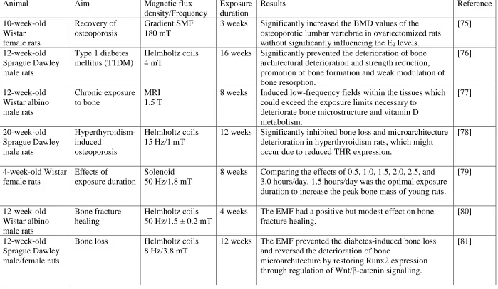
1.2.3 Animal studies

Few clinical studies concern EMF therapy, but animal studies have been carried out to determine the effectiveness of EMF on bone growth. These studies indicate that EMF can contribute to bone formation and healing process in various manners of magnetic flux density, frequency and exposure duration. Representative animal studies in recent years are summarised in Table 1 and generally show some positive effects.

(24)

12

uniform electromagnetic exposures, but there are discrepancies between the set of magnetic flux density and frequency. Hence, researchers argued that the controversial effects of EMF on biological objects were due to experiments not carried out in well-defined conditions [50]. Extensive studies have been done to categorise the parameters of EMF for optimal laboratory settings [51]. EMF signal induces electric and magnetic signal to initiate a cascade of biochemical reactions [52]. The EMF stimulation is characterised by factors such as magnetic field intensity, waveform, dose-response pattern [53], exposure duration [54], localisation of stimulation and spatial orientation of the exposure system [55]. Other factors can influence the response to magnetic field exposure by frequency and modulation, field uniformity, a combination of coil system and precise placement, field intensity and polarisation, noise, vibration and temperature of conducting materials, voltage carrying wires and metal equipment, construction materials and the experiment schedule [56]. Therefore, EMF parameters are proposed to be considered prior to evaluating the effect of magnetic field on a biological sample in aspect of (i) type of magnetic fields, (ii) magnetic flux density, (iii) frequency, (iv) exposure duration, (v) pulse shape, (vi) spatial gradient (dB/dx) and temporary gradient (dB/dt) [57].

1.3.1 Mechanisms of EMF on biological systems

(25)

13

[60]. These electrical signals in the form of minute electric currents flow around and within the cells and are of critical importance for their normal functioning and can accelerate normal cellular function such as endocytosis [61]. EMF perturb these currents and charges and positively influence the process of cellular functioning. It has been suggested that EMFs may trigger specific, measurable cellular responses such as DNA synthesis, transcription, and protein synthesis by altering or augmenting pre-existing endogenous electrical fields [62]. This mechanism adds further evidence to the fact that external non-invasive electric stimulation is a potent tool in augmentation of cells, tissue and organs. A well-established phenomenon in physics, ion cyclotron resonance (ICR) and ion parametric resonance (IPR) models were proposed, which state that ions resonate when exposed to a specific combination of alternating and static magnetic fields [63]. Hall effect may provide the electrical basis of EMF in the bone lacuna canalicular system, which attaches the positive ions at the negative interface of the bone matrix [64]. When EMF is applied, the moving charged particles encounter a Lorentz fore perpendicular to their direction. Cations accumulate at the downward surface, and anions go upward to forming a hall voltage [65].

(26)

14

However, an argument exists against Lorentz forces in cells since dielectric media and plasma lack moving charges [69]. Buchachenko and Kuznetsov [70] emphasised the molecular radical pair paradigm as a reliable basis for understanding and deliberately using biochemical magnetic effects in medicine. Biochemical processes are accompanied by generation or participation of ion-radicals in pairs. Radical pair mechanism implies that two radicals are produced simultaneously with paralleled or anti-paralleled electron spins. Chemical reactions are spin selective which are allowed only for those spin states of reactants with identical total spins. The spin states of the pair, singlet and triplet are different in chemical reactivity but identical in structure. In triplet state, the reactions are forbidden. Weak magnetic interaction might provide a manner to overcome the spin prohibition of processes in biochemistry. Magnetic interactions induce singlet-triplet spin conversion and switch over the reaction between spin-allowed and spin-prohibited channels, controlling the reaction pathways and chemical reactivity. Radical pair mechanism has been shown functionally on the molecular level in biochemical reactions [71]. Three types of magnetic interactions are considered for catalysing chemical and biochemical reactions, namely Zeeman interaction, Fermi interaction and microwaves. Magnetic catalysis is controllable and switchable by using magnetic isotopes or paramagnetic ions [72]. The magnetic interaction effects on the enzymatic ATP synthesis were detected for the creatine kinase in vitro [73]. The magnetic control of enzymatic DNA synthesis was observed in time-varying magnetic fields [74].

(27)

[image:27.842.121.820.113.520.2]

15 Table 1-1 Animal studies

Animal Aim Magnetic flux

density/Frequency

Exposure duration

Results Reference

10-week-old Wistar female rats Recovery of osteoporosis Gradient SMF 180 mT

3 weeks Significantly increased the BMD values of the osteoporotic lumbar vertebrae in ovariectomized rats without significantly influencing the E2 levels.

[75]

12-week-old Sprague Dawley male rats

Type 1 diabetes mellitus (T1DM)

Helmholtz coils 4 mT

16 weeks Significantly prevented the deterioration of bone architectural deterioration and strength reduction, promotion of bone formation and weak modulation of bone resorption. [76] 12-week-old Wistar albino male rats Chronic exposure to bone MRI 1.5 T

8 weeks Induced low-frequency fields within the tissues which could exceed the exposure limits necessary to

deteriorate bone microstructure and vitamin D metabolism. [77] 20-week‐old Sprague Dawley male rats Hyperthyroidism‐ induced osteoporosis Helmholtz coils 15 Hz/1 mT

12 weeks Significantly inhibited bone loss and microarchitecture deterioration in hyperthyroidism rats, which might occur due to reduced THR expression.

[78] 4-week-old Wistar female rats Effects of exposure duration Solenoid 50 Hz/1.8 mT

8 weeks Comparing the effects of 0.5, 1.0, 1.5, 2.0, 2.5, and 3.0 hours/day, 1.5 hours/day was the optimal exposure duration to increase the peak bone mass of young rats.

[79] 12-week-old Wistar albino male rats Bone fracture healing Helmholtz coils 50 Hz/1.5 ± 0.2 mT

4 weeks The EMF had a positive but modest effect on bone fracture healing.

[80]

12-week-old Sprague Dawley male/female rats

Bone loss Helmholtz coils 8 Hz/3.8 mT

12 weeks The EMF prevented the diabetes-induced bone loss and reversed the deterioration of bone

microarchitecture by restoring Runx2 expression through regulation of Wnt/β-catenin signalling.

(28)

16

Chapter 2

(29)

17 2.1 Bone modelling and remodelling

Bone is a continuously updated tissue and constituted mainly by BMSCs, osteoblast, osteocytes and osteoclasts. The dynamic balance between bone formation and resorption, such as bone modelling and remodelling, has a pivotal role to play in the normal bone metabolism, bone integrity and appropriate bone strength [82]. Bone modelling and remodelling are both involved in osteogenesis and skeletal growth. Bone modelling is characterised by the process of bone formation and resorption with a net increase in bone mass. The mechanism involves activation-formation and activation-resorption, which primarily occurs in childhood [83]. Activation is signalled by local tissue strain and involves the recruitment of progenitor cells that differentiate into mature osteoblasts or osteoclasts. Once the appropriate cell population is activated, the processes of formation and resorption happen until sufficient bone mass is altered for normalising local strains. In contrast, bone remodelling is defined as renewing and maintaining bone in which a coupled process occurs between the catabolic effects of bone-resorbing osteoclasts and anabolic effects of bone-forming osteoblasts [84]. During a bone remodelling process, bone mass is removed at sites where the mechanical loads are low, while bone is formed where mechanical stimuli are transmitted repeatedly.

(30)

18

site of the BMU [86]. Vascularisation and angiogenesis are prerequisites for bone formation and remodelling. They serve multiple purposed bone cell progenitors via blood capillaries to establish the modelling and remodelling site. The blood supply also allows the BMU to become accessible to immune cell infiltration and interaction with bone cells.

Bone remodelling involves the balance between osteoclast and osteoblast activity, which is regulated by numerous signalling pathways [87]. Deregulation of signalling pathways in bone cells may lead to bone diseases such as osteoporosis and osteoarthritis. In the big picture, osteoblasts facilitate bone formation by laying down a matrix which subsequently is mineralised, and produce receptor activator of nuclear factor- B ligand (RANKL) initiating osteoclastogenesis [88]. Osteoclasts, activated

by proinflammatory cytokines and RANKL/macrophage colony stimulating factor (M-CSF), initiate bone resorption by releasing catalytic enzymes like Cathepsin K (Cat K) and matrix metalloproteases (MMPs) in a resorptive pit formed on the bone surface [89]. Protection against bone damage can be achieved by (i) inhibiting RANKL production by increasing the production of osteoprotegerin (OPG), (ii) suppressing the proinflammatory cytokines, (iii) inhibiting production of Cat K and MMPs, and (iv) inhibiting osteoclast formation. The cellular coupling between osteoblasts and osteoclasts is complex and is massively coordinated by several regulatory systems to keep both remodelling and resorption processes synchronised. The accentuation of one or the other process eventually leads to bone fragility and clinical diseases of the skeleton, such as osteoporosis, arthritis and osteolysis [90].

2.1.1 Osteoblast

(31)

19

musculoskeletal tissues such as cartilage, fat, muscle, ligament and tendon [91]. The commitment of these stem cells to the osteoblast lineage is highly driven by the growth factors wingless-type proteins (Wnts) and bone morphogenetic proteins (BMPs). Once skeletal stem cells are committed to the osteoblast lineage, the proliferation of osteoblast precursor cells begins. These cells produce type I collagen for the basic building block of bone, osteocalcin and alkaline phosphatase for mineral deposition. Osteoblast precursor cells mature into cuboidal osteoblasts. Besides their role in bone formation, the osteoblasts are involved in the recruitment and maintenance of osteoclasts by expressing M-CSF, RANKL and OPG [92]. Mature osteoblasts may undergo apoptosis or coalesce into the heterogeneous population bone-lining cells, or eventually become encased and trapped within the matrix to become osteocytes. The proportion of osteoblasts following each possibility varies in all mammals and is not conserved among different types of bone. The age of the mammal may also influence the number of osteoblasts that transform into osteocytes [93].

2.1.2 Osteoclast

(32)

20

precursors, controlling their formation and the activity of bone resorption [97]. The osteoclasts serve as bone-resorbing cells by eroding bone, enabling the tissue to be remodelled during growth and in response to stresses. Bone resorption is an essential event during bone growth, tooth eruption, fracture healing and the maintenance of blood calcium level. Osteoclasts are derived from hematopoietic stem cells [98] and are created by the differentiation of monocyte/macrophage precursor cells at or near the bone surface [99]. Hence, osteoclasts share a common pathway with that of macrophage and dendritic cells [100].

2.1.3 Gene network between osteoblasts and osteoclasts

Critical to maintaining the strength of bone, the process of bone remodelling must be tightly regulated [83]. Thus, bone mass and structure are ultimately the consequence of interactions of multiple pathways in the network that are modulated by hormonal, cytokine and immune systems. This control is exquisitely sensitive to external stimuli such as EMF [101, 102]. In vitro studies clearly show that a variety of molecules in bone metabolism are affected by EMF application, including BMP-2, TGF-β and

IGF-II [103, 104] (Figure 2.1). EMFs resulted in the activation of the extracellular signal-regulated kinase (ERK), mitogen-activated protein kinase (MAPK) and prostaglandin

synthesis, which may also lead to stimulatory effects on bone [105, 106].

(33)

21

(34)

22

conceptual block diagram using data and text mining in Figure 2.2. Established knowledge from feedback control of dynamic systems in engineering, allows us to define four primary functions for known regulations: induce, inhibit, relate, and complex. These primary functions enable construction of a network with systematic loops.

2.2 Mathematical models for simulating cell growth and movement

Efforts for modelling mechanism of EMF on bone remodelling have focused on mechanical functions or biological functions based on signalling pathways [122, 123]. Mathematical models of bone remodelling have been established on the RANK/RANKL/OPG pathway under the influence of PTH, mechanical force, and EMF at the cellular level [124-126]. These models can be extended to different waveforms of EMF and other external perturbation [127, 128].

(35)

23

In order to remove the limitations to generalisation concerning causes and effects of bone remodelling under PEMF, mathematical models provide a dynamic, quantitative and systematic description of the relationships among interacting components of the biological system [138]. Kroll [139] and Rattanakul, et al. [140] each proposed a mathematical model accounting for the differential activity of PTH administration on bone accumulation. Komarova, et al. [141] presented a theoretical model of autocrine and paracrine interactions among osteoblasts and osteoclasts. Komarova [142] also developed a mathematical model that describes the actions of PTH at a single site of bone remodelling, where osteoblasts and osteoclasts are regulated by local autocrine and paracrine factors. Potter, et al. [143] proposed a mathematical model for the PTH receptor (PTH1R) kinetics, focusing on the receptor’s response to PTH dosing to discern bone formation responses from bone resorption. Lemaire, et al. [144] incorporated detailed biological information and a RANK-RANKL-OPG pathway into the remodelling cycle of a model that included the catabolic effect of PTH on the bone, but the anabolic effect of PTH was not described. Based on the Lemaire’s model, Wang, et al. [145] developed a mathematical model that could simulate the anabolic behaviour of bone affected by intermittent administration of PTH, as well as a theoretical model and its parametric study of the control mechanisms of bone remodelling under the mechanical stimulus. Pivonka, et al. [146], [147] extended the bone-cell population model based on the Lemaire’s model to explore the model structure of cell-cell interactions theoretically and then investigated the role of the RANK-RANKL-OPG system in bone remodelling.

(36)

24

stimulus [155]. FEM is successful in analysing the macroscopic level of bone structure, especially in studying microcracks [156] and reconstruction of bone models from CT images [157, 158]. Such problems can refer to similar studies from material research [159-165]. Although the FEM may put forward the quantitative prediction of cell behaviours, it is not clear exactly how mechanical loading affect the activities of osteoblasts and osteoclasts in each cell cycle. Besides, the parametric simulation of cell signalling introduces unknowns into the model and raises a question of how signalling pathways interact with each other instead of the answer for the coupling mechanism between activities of osteoblasts and osteoclasts at the cellular level. It might be feasible to describe each component mathematically on a small scale of signalling (Figure 2.1), while the mission is impossible for a signalling network (Figure 2.2). Further, Spatial and temporal heterogeneity of molecules or proteins require a comprehensive mathematical description instead of connecting signalling pathways with simple positive and negative circuit feedbacks.

(37)

25

and electromagnetic fields gain significance in the therapy of bone fracture healing and bone disease [169].

(38)

26

[image:38.595.119.520.73.407.2]

(39)

(40)

28

(41)

29

Chapter 3

(42)

30 3.1 Research question

Researchers have been confused about the effect of EMF on a biological system in past decades. Chapter 1 has shown the efforts to elucidate one or several factors for explaining the underlying mechanism of the EMF effect on a biological system. Nevertheless, we realise that different dataset yield contradictions when articulating them into one picture. In classical physics, data obtained by using various instruments supplement each other and can be combined into a consistent picture where the influence of the measuring procedure can easily be subtracted from its outcome. On the contrary, the effect of EMF on cells illustrates that changing the experimental arrangement is equivalent to changing the holistic phenomena. Consequently, we could not predict the effect of EMF on the experiment results even though numerous similar experiments have been carried out.

(43)

31

Different pieces of information are taken into being mutually exclusive, yet jointly indispensable to characterise a specific object. We write research questions here about the consistency of bone cells’ bio-data in weak EMF.

• In the same experimental setting except for magnetic intensity, whether the relationship between osteoblasts population and magnetic intensity follows the same pattern throughout the time.

• In the different types of EMFs but with a similar scale of magnetic intensity, whether the relationship between osteoblasts population and magnetic intensity obeys the same principle.

• Whether the principle derived from osteoblasts behaviour in weak EMF is consistent in the co-culture of osteoblasts and osteoclast.

3.2 Hypothesis

The primary hypothesis assumes that EMFs can affect the movement of osteoblasts. The mechanisms of EMFs on biological systems in Chapter 1 provide this hypothesis with substantial evidence. However, it is an open question of how to describe the movement of osteoblasts mathematically. We prefer the concept of “cell probability” which means the chance that cells appear at a specified location by counting the number of cells at a specified location in a particular time and then taking the ratio of this number to the total number during that time.

(44)

32

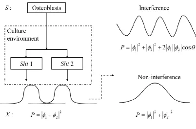
We imagine the effects of EMF on cell probability as a slit, which is a derivative model of the double-slit experiment (Figure 3.1). The culture environment consists of at least two slits, with and without EMF. When osteoblasts are cultured in EMFs, the cell probability has two possible patterns after passing through slits. Therefore, the superposition of probability amplitudes could occur. We write the probability amplitude as

Cell final at Cell initial at x s

= . (3.2.1)

Following the expression in physics, the right part to the vertical line gives the initial condition, and the one on the left indicates the final condition. The abbreviation of (3.2.1) is

x s

 =

. (3.2.2)

Such an amplitude might be a complex number. Each replicate in cell culture has the same probability amplitude rather than the cell population. If a factor is amplified in the culture environment such as hormones, this will create a new slit. We mark the two slits as 1 and 2. The resultant amplitude is calculated by multiplying in succession the amplitude for each of the successive events,

1 1 2 2

x s = x s + x s , (3.2.3)

which equals to

1 2

  = + . (3.2.4)

The cell probability P is given by

2

P=  . (3.2.5)

(45)

33

2 2 2

1 2 1 2 2 1 2 cos

P=  + =  +  +   , (3.2.6)

where



is the phase difference between



1 and



2. If an experiment is performed

with the capability of determining whether one or another alternative is taken, the interference is lost,

2 2 2

1 2 1 2

P=  + =  + . (3.2.7)

For instance, screening tests in biological experiments are taken without interference. When a PEMF is specified in magnetic intensity and frequency, we calculate a much more complicated problem. In physics, when an event can occur in several alternative ways, the probability amplitude for the event is the sum of the probability amplitudes for each way considered separately. We build two filters for PEMF, where the first filter represents the magnetic intensity and the second filter represents the frequency. If the first filter has i slits and the second filter have j slits, the complete amplitude is written by

j i

x s =



x j j i i s . (3.2.8)

When osteoclasts appear in the experiment, the disturbance happens between osteoclasts and the slits. The amplitude of osteoblasts is described in the equation (3.2.3). The amplitude

1 s

occurs when osteoblasts go from

s

to slit 1 and multiply the amplitude a when osteoblasts contact with osteoclasts at slit 1. Then the amplitude that osteoblast go from s to x via slit 1 and contact osteoclasts is

1 1 1

a = x a s . (3.2.9)

Similarly, the amplitude that osteoblasts go via slit 2 and contact osteoclasts is

2 2 2

(46)

34 The probability of both amplitudes is

2

1 2

P= a +b , (3.2.11)

(47)

[image:47.595.119.522.73.337.2]

35

(48)

36

Chapter 4

(49)

37 4.1 Materials

4.1.1 Chemical reagents

Chemical reagents involved in experiments conducted in this thesis were of analytical grade unless indicated otherwise and were purchased from the following manufacturers:

Description Manufacturer

1α,25-dihydroxyvitamin D3 Sigma-Aldrich, USA

4-(2-hydroxyethyl)-1-piperazineethanesulfonic acid (HEPES)

ThermoFisher, Australia

α-MEM (α-modification of Eagle’s medium) Life Technologies, Australia

β-mercaptoethanol Sigma-Aldrich, USA

Alizarin red S Biochemicals Inc, USA

Bovine serum albumin Sigma-Aldrich, USA

Bromophenol blue Bio-Rad, USA

Chloroform ThermoFisher, Australia

Dexamethasone Sigma-Aldrich, USA

Dimethyl Sulphoxide (DMSO) ThermoFisher, Australia D-MEM (Dulbecco’s-modification of Eagle’s

medium)

Life Technologies, Australia

Ethanol (100%) EMD Millipore Corporation, USA

FBS (Foetal Bovine Serum) Life Technologies, Australia Hanks’ balanced salt solution Life Technologies, Australia HEPES (

4-(2-hydroxyethyl)-1-piperazineethanesulfonic acid)

(50)

38

L-ascorbic acid phosphate Sigma-Aldrich, USA

L-Glutamine Sigma-Aldrich, USA

Liquid nitrogen (N2) Air Liquid, Australia

Penicillin Life Technologies, Australia

Skim Milk Powder Standard supermarket brand

Sodium chloride (NaCl) Bio-Rad, USA

Sodium dodecyl sulphate (SDS) Bio-Rad, USA Sodium hydroxide (NaOH) Sigma-Aldrich, USA Sodium phosphate dibasic (Na2HPO4) Sigma-Aldrich, USA Sodium phosphate monobasic (NaH2PO4) Sigma-Aldrich, USA

Tween-20 Bio-Rad, USA

4.1.2 Commercial kits and molecular products

10 x Reaction Buffer, 1 mL of 200 mM Tris-HCl, pH 8.3, 20 mM MgCl2

Sigma-Aldrich, USA

5 x First Strand Buffer Invitrogen, USA

Amplification Grade DNAse I ThermoFisher, Australia BD Pharm LyseTM red cell lysis buffer (10 x) BD Bioscience, USA DAPI (4’,6-diamidino-2-phenylindole),

dilactate

Biotium, USA

Fastlane Cell cDNA Kit QIAGEN Gmbh, Australia

RNEasy Mini kit QIAGEN Gmbh, Australia

(51)

39 4.1.3 Other products and consumables

0.2 mL PCR Tubes ThermoFisher, Australia

50 mL Centrifuge Tubes ThermoFisher, Australia

BD 1 mL Syringe BD Bioscience, USA

BD PrecisionGlideTM Needles 25 G BD Bioscience, USA Coverslips-round 5 mM, 22×22 mm2 and

22×40 mm2

Knittle Glaser, Germany

Filter Paper Whatman International, UK

Glass Slides Knittle Glaser, Germany

Parafilm Laboratory Film Merck Millipore, Australia

Transfer pipettes Sigma-Aldrich, USA

4.1.4 Cytokines

Recombinant human macrophage-colony stimulating Factor (M-CSF)

EMD Millipore Corporation, USA

Recombinant human soluble RANK ligand (sRANKL)

EMD Millipore Corporation, USA

4.1.5 Solutions

(52)

40

Solution Composition and preparation

Flow cytometry wash buffer PBS containing 1% FBS and 0.1% (w/v) sodium azide, stores at 40C.

Phosphate buffered saline (PBS)

10 x PBS stock solution in ddH2O: 70 mM Na2HPO4, 30 mM NaH2PO4 and 1.3 M NaCl. 1 x PBS:1 in 10 dilutions of 10 x PBS stock solution and calibrated to pH 7.4.

SDS-PAGE running buffer 10x stock solution in ddH2O: 25 Trizma base, 1.92 M glycine and 1% (v/v) SDS. 1 x working solution: 1in 10 dilutions of the 10x stock solution in ddH2O. SDS-PAGE sample loading

buffer

4x stock solution dissolved in ddH2O:240 mM Tris-HCl (pH 6.8), 8% (w/v) SDS, 40% (v/v) glycerol, 0.04% (w/v) bromophenol blue and 5% (v/v) β-mercaptoethanol. Stored at 4 0C.

SDS-PAGE separating gel buffer

1.5 M Tris-HCl (pH 8.8) and 0.4% (w/v) SDS prepared inddH2O.

SDS-PAGE stacking gel buffer

1 M Tris-HCl (pH 6.8) and 0.4% (w/v) SDS dissolved inddH2O.

Sodium deoxycholate solution

10% (w/v) solution dissolved in ddH2O.

Tartrate-resistant acid phosphatase (TRAP) stain

(53)

41

TRAP stain solution A 100 mM sodium acetate trihydrate, 50 mM sodium tartrate dihydrate and 0.22% (v/v) glacial acetic acid. Adjusted to pH of 5.0.

Western blot transfer buffer 25 mM Trizma base, 192 mM glycine and 10% (v/v) methanol in ddH2O.

4.1.6 Equipment

4300 SE/N Schottky Field Emission Electron Microscopy

Hitachi, Japan

96-well Thermal Cycler Applied Biosystems, USA Automatic CO2 Incubator Thermo Scientific, USA Digital Teslameter with the Probe 3B Scientific, Germany Eclipse TE2000s Fluorescent Microscope Nikon Instruments Inc., USA

Function Generator 3B Scientific, Germany

ImageQuant LAS 4000 GE Healthcare, USA

MiniSpin® microcentrifuge Eppendorf AG, Germany MilliQ Water System Millipore Corporation, USA Nanodrop® ND-1000 UV-Vis

Spectrophotometer V3.3

Thermo Scientific, USA

Nikon CoolPix S4 Digitial Camera Nikon Corp., Japan

(54)

42 4.1.7 Software

ANSYS Ansys, Inc. USA

FACSDiva BD Biosciences, USA

Microsoft Research Image Composite Editor Microsoft, USA

MATLAB MathWorks, USA

FlowJo FlowJo LLC, USA

Prism GraphPad Software, USA

Origin OriginLab, USA

4.1.8 RT2 profiler PCR array

The PCR array catalogue is PAHS-026z.

Symbol Description

ACVR1 Activin A receptor, type I AHSG Alpha-2-HS-glycoprotein

ALPL Alkaline phosphatase, liver/bone/kidney ANXA5 Annexin A5

BGLAP Bone gamma-carboxyglutamate (gla) protein

BGN Biglycan

(55)

43

BMPR1A Bone morphogenetic protein receptor, type IA BMPR1B Bone morphogenetic protein receptor, type IB BMPR2 Bone morphogenetic protein receptor, type II CALCR Calcitonin receptor

CD36 CD36 molecule (thrombospondin receptor) CDH11 Cadherin 11, type 2, OB-cadherin (osteoblast) CHRD Chordin

COL10A1 Collagen, type X, alpha 1 COL14A1 Collagen, type XIV, alpha 1 COL15A1 Collagen, type XV, alpha 1 COL1A1 Collagen, type I, alpha 1 COL1A2 Collagen, type I, alpha 2 COL2A1 Collagen, type II, alpha 1 COL3A1 Collagen, type III, alpha 1 COL5A1 Collagen, type V, alpha 1

COMP Cartilage oligomeric matrix protein CSF1 Colony stimulating factor 1 (macrophage)

CSF2 Colony stimulating factor 2 (granulocyte-macrophage) CSF3 Colony stimulating factor 3 (granulocyte)

CTSK Cathepsin K

DLX5 Distal-less homeobox 5 EGF Epidermal growth factor

(56)

44 FGF2 Fibroblast growth factor 2 (basic) FGFR1 Fibroblast growth factor receptor 1 FGFR2 Fibroblast growth factor receptor 2

FLT1

Fms-related tyrosine kinase 1 (vascular endothelial growth factor/vascular permeability factor receptor)

FN1 Fibronectin 1

GDF10 Growth differentiation factor 10 GLI1 GLI family zinc finger 1

ICAM1 Intercellular adhesion molecule 1

IGF1 Insulin-like growth factor 1 (somatomedin C) IGF1R Insulin-like growth factor 1 receptor

IGF2 Insulin-like growth factor 2 (somatomedin A) IHH Indian hedgehog

ITGA1 Integrin, alpha 1

ITGA2 Integrin, alpha 2 (CD49B, alpha 2 subunits of VLA-2 receptor)

ITGA3

Integrin, alpha 3 (antigen CD49C, alpha 3 subunits of VLA-3 receptor)

ITGAM Integrin, alpha M (complement component 3 receptor 3 subunit)

ITGB1

Integrin, beta 1 (fibronectin receptor, beta polypeptide, antigen CD29 includes MDF2, MSK12)

MMP10 Matrix metallopeptidase 10 (stromelysin 2)

MMP2

Matrix metallopeptidase 2 (gelatinase A, 72kDa gelatinase, 72kDa type IV collagenase)

(57)

45 MMP9

Matrix metallopeptidase 9 (gelatinase B, 92kDa gelatinase, 92kDa type IV collagenase)

NFKB1 Nuclear factor of kappa light polypeptide gene enhancer in B-cells 1

NOG Noggin

PDGFA Platelet-derived growth factor alpha polypeptide

PHEX Phosphate regulating endopeptidase homolog, X-linked RUNX2 Runt-related transcription factor 2

SERPINH1

Serpin peptidase inhibitor, clade H (heat shock protein 47), member 1, (collagen binding protein 1)

SMAD1 SMAD family member 1 SMAD2 SMAD family member 2 SMAD3 SMAD family member 3 SMAD4 SMAD family member 4 SMAD5 SMAD family member 5

SOX9 SRY (sex determining region Y)-box 9 SP7 Sp7 transcription factor

SPP1 Secreted phosphoprotein 1

TGFB1 Transforming growth factor, beta 1 TGFB2 Transforming growth factor, beta 2 TGFB3 Transforming growth factor, beta 3

TGFBR1 Transforming growth factor, beta receptor 1

TGFBR2 Transforming growth factor, beta receptor II (70/80kDa) TNF Tumour necrosis factor

(58)

46 TWIST1 Twist homolog 1 (Drosophila) VCAM1 Vascular cell adhesion molecule 1

VDR Vitamin D (1,25- dihydroxy vitamin D3) receptor VEGFA Vascular endothelial growth factor A

VEGFB Vascular endothelial growth factor B ACTB Actin, beta

B2M Beta-2-microglobulin

GAPDH Glyceraldehyde-3-phosphate dehydrogenase HPRT1 Hypoxanthine phosphoribosyltransferase 1 RPLP0 Ribosomal protein, large, P0

HGDC Human Genomic DNA Contamination RTC Reverse Transcription Control

PPC Positive PCR Control

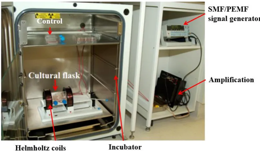
4.2 PEMF apparatus design

Self-made EMF device was used in controlling the frequency and signal type (

Figure 4.1). The EMF Apparatus consists of two tubes (Figure 4.2), one protective shield, one platform (Figure 4.3) and two supports (Figure 4.4), generating PEMF signal and magnetic field strength by Helmholtz coils or solenoid of around 300 turns copper wires each. This apparatus also includes a digital oscilloscope and teslameter for measurement.

4.3 Culture and in vitro studies of Sao-2 cell line

(59)

47 4.3.1 Saos-2 cell line

Saos-2 (sarcoma osteogenic) was purchased from Australian agent (Sigma Aldrich, catalogue number: 89050205), which was a non-transformed cell line derived from human primary osteogenic sarcoma of an 11-year old female Caucasian. The Saos-2 cell line was from the ECACC collection, used as a permanent line of human osteoblast-like cells and a source of bone-related molecules.

4.3.2 Initiation of the culture process

The medium of 5 mL was pre-equilibrated within a 25 cm2 culture flask for 2 hours in an incubator. Saos-2 cells were removed from frozen storage and thawed in a 37 0C water bath with agitation. The cryovial was removed when the ice melted and then rinsed with 70% ethanol. The cells were resuspended and transferred to a 25 cm2_flask with 5 mL equilibrated medium, then incubated 30 minutes for the settlement. The cells were rinsed with 5ml of warmed fresh medium to remove the cryoprotectant. The cells were cultured in fresh media and monitored daily for use. Saos-2 cells could grow in a stationary flask using medium supplemented with 10% FBS, 2 mM L-glutamine and 0.01% kanamycin. The cells were kept in a 2 mm medium layer in a flask with the caps opening a quarter turn to balance the aeration and nutrition.

4.3.3 SubcultureSaos-2

(60)

α-48

MEM of 2 mL supplemented with 10 ng/mL MCSF and cultured in culture flasks or plates.

4.3.4 Count cell densities of Saos-2 cells

The cells of 100 µL were transferred to a well in a 96-well plate with 10 µL sterile 0.4% trypan blue. The mixture was ensured homogenous and transferred 10 µL to the haemocytometer. The dead cell was counted in the colour of blue and divided by the total number of cells for the proportion of dead or lysed cells. The viability was one minus the proportion of dead cells.

4.3.5 Cryopreservation and retrieval of cultured cells

The cells were frozen when exceeding 80% in confluence. The cells were gently dislodged and centrifuged for 6 minutes at 300 x g. The cell pellet was resuspended to 5-6 x106 cells/mL and added 10% DMSO. Plastic cryovials were loaded with a cell suspension of 1 mL. The vials were placed on ice tub for 15-30 minutes to allow equilibration of the cells with the DMSO-containing medium. The vials were transferred to the tray of the cell freezer and adjusted the height of the ray according to the manufacturer’s instructions. The freezing unit was inserted in the neck of the liquid nitrogen refrigerator for approximately 3 hours. Transfer frozen vials were transferred to a storage canister in liquid nitrogen.

(61)

49

was to immerse frozen vials in a warm water bath (37-40 0C) so that the cells thawed in about 1.5 minutes.

4.4 Isolation, culture and in vitro studies of human osteoblasts 4.4.1 Isolation and culture of osteoblasts from human trabecular bone

Pieces of excised human bone specimens were placed in sterile saline or PBS at time of collection, and the samples were transferred in a foam box without ice. Completed α-MEM (α-MEM supplemented with 10% FBS, 2 mM L-glutamine, 100 U/mL Penicillin and 100 µg/mL Streptomycin) and filtered PBS were warmed in 37 0C water bath. The centrifuge was set at 300 x g, 4 0C and 6 minutes. Aseptic technique was used to cut the bone specimen into small pieces about 1-2 mm using a scalpel blade or scissors. The bone chips were washed five times with sterile PBS and transferred into a sterile Falcon tube. Contaminating red blood cells were removed using a vortex mixer. 8-10 pieces of bone were placed into a T75 flask along with 20 mL completed α-MEM. The flask was placed in an incubator with 5% CO2 at 37 0C. After 1 week, the medium was removed, and fresh culture medium was added. The bone pieces were cultured for another week without disturbing. After that, the culture medium was changed every 2 days. Between 3-4 weeks the cells could be confluent about 1-2 x 106 cells/flask.

4.4.2 Harvest of monolayer cultures

(62)

50

solution was centrifuged at 300 x g, 4 °C for 6 minutes, and the supernatant was disposed. α-MEM of 3 mL was added to the flask for the cell suspension. A pipette was used to break cell clusters by pressing the tip of the pipette against the bottom of the flask. The cell suspension was passed through a needle of 10 mL syringe 5-6 times with the needle bevel pressing against the tube wall to further separate the cells.

4.4.3 In Vitro osteoblasts cell mineral formation assay

(63)

51

4.5 Induction and culture of human osteoclasts 4.5.1 Preparation of solution

Osteoclast cells can be differentiated from human peripheral blood mononuclear cells (PBMCs) using differentiating culture medium. HANK’s solution was prewarmed in a water bath at 37 0C and filtered using a filter cup (0.2 µM) before use. Completed osteoclast culture medium was made by α-MEM supplemented with 1% L-Glutamine, 10% FCS, 1% PSN, 10-8 M Dexamethasone, 10-8 M Vitamin D3 and 25 ng/mL M-CSF. DMSO was used to dissolve Vitamin D3. Human recombinant RNAKL was prepared at 50 ng/mL.

4.5.2 PBMC isolation

The Buffy coat 15 mL in a falcon tube and 20 mL pre-warmed HANKs was added to dilute the buffy coat. Ficoll-Paque of 7.5 mL was added to an empty 50 mL Falcon tube, and diluted buffy coat of 10 mL was loaded over Ficoll solution using a syringe. The ratio of Ficoll and diluted buffy coat was 3:4. After loading, all of the tubes were placed on a centrifuge, spun at 500 x g, 25 C for 30 minutes. The mononuclear cells (PBMCs) were collected at the interface using a sterile pipette directly inserted into the PBMCs layer. This layer was like a cake in between orange colour and white colour. The PBMCs were transferred to a fresh 50 mL falcon tube. Cells were washed with 20 mL HANKs and centrifuged at 500 x g, 25 C for 5 minutes. The supernatant was discarded and completed osteoclast cell culture medium was added to make 5-10 mL cell suspension, depending on how many cells isolated.

4.5.3 PBMC cell culture

(64)

52

The cells were counted under bright field microscopy. For example, seeding to 24-well plate and the cell suspension was 0.5 mL/well, the volume of cell seeding suspension was 12 mL. The cell seeding suspension was made by adding the above volume into 14 mL completed osteoclast cell culture medium. Cell seeding suspension of 0.5 mL was added to each well of a 24-well plate. The cells were incubated at 37 0_{C, 5% CO}

2

and 95% moisture incubator. In day 4, the culture medium was changed. In day 7, the culture medium was changed with adding human recombinant RANKL into the cell culture to induce osteoclasts. The final concentration of RANKL in the culture media was 50 ng/mL. In day 10, the osteoclasts could be observed under bright field microscopy.

4.5.4 TRAP staining

(65)

53 4.5.5 Flow cytometer and analysis

The FACSCalibaur, FACSCanto II and LSR Fortessa TM SORP were used for flow cytometric studies. FACSDiva software was used for application setup, data acquisition and data compensation. The live and single mononuclear cells were gated using Forward Scatter (FSC) and Side Scatter (SSC) plots. Events were recorded. Acquired and compensated data was imported into FlowJo for analysis.

4.6 Western blotting

Western blotting allows the specific detection of proteins on membranes after separation by SDS-PAGE. It combines the resolution of gel electrophoresis with the specificity of immunochemical detection. This technique is beneficial for the identification and semi-quantification of specific proteins in complex mixtures of proteins.

4.6.1 Protein extract and assay

(66)

54

were assayed in duplicate or triplicate. The standard and sample solution of 10 μL each were put into separate microliter plate wells. Diluted dye reagent of 200 μL was added to each well. The sample and reagent were mixed thoroughly using a microplate mixer. The mixture was incubated at room temperature for at least 5 minutes. Since absorbance could increase over time, samples should incubate at room temperature for no more than 1 hour. Measure absorbance was at 595 nm.

4.6.2 Blotting and detection

(67)

55

was washed three times with Basic Buffer on the shaker for 10 minutes each time. Primary antibody was diluted with Primary Antibody Dilution Buffer. The membrane was incubated with the diluted primary antibody on a shaker for 1 hour at room temperature. The membrane was then washed three times with Washing Buffer on the shaker for 10 minutes each time. The secondary antibody was diluted with Primary Antibody Buffer containing 5% dry milk. The membrane was incubated with the diluted secondary antibody on a shaker for overnight at 4 0C. The membrane was then washed three times with Washing Buffer on the shaker for 10 minutes each time. The detection reagents were taken from the storage at 4 0C and equilibrated to room temperature before opening. Detection solutions were mixed to the final volume of 0.1 mL/cm2. Protein side of the washed membrane was placed upon a transparency film. The mixed detection reagent was added on the membrane for a reaction of 3 minutes at room temperature. The reagents covered the entire surface of the membrane, held by surface tension on to the surface of the membrane. Excess detection agent was drained off by holding the membrane gently in forceps and touching the edge against a tissue. The membrane ‘protein-side’ was placed facing the camera. Blots were exposed to GE Healthcare ImageQuant LAS 4000 at least three different exposures.

4.7 RNA extraction and quantification

(68)

56

(69)

[image:69.595.121.541.119.363.2]

57

(70)

58 (A)

[image:70.595.178.445.101.600.2]

(B)

(71)

59 (A)

[image:71.595.119.502.98.543.2]

(B)

(72)

60 (A)

[image:72.595.156.455.83.617.2]

(B)

(73)

61

Chapter 5

(74)

62 5.1 Introduction

The hypothesis in Chapter 3 describes the qualitative response of bone cells to EMFs. The EMFs as an external stimulus alter the original environment of cell culture. In this chapter, we attempt to establish several frameworks for quantitatively interpreting the evolution of cell probability under a general situation of external stimulus. The frameworks involve two major components, (i) an external stimulus and (ii) the cellular response to the stimulus. The response is in two steps, (i) the detection of the stimulus and (ii) the transduction of the stimulus into the controls of cellular interaction. Ideally, each cell is distinguished from their direction of motion, reorientation frequency and step length between reorientations in response to the stimulus. However, the coupling between cell density and the local stimulus intensity might prevent the process of distinguishing. For example, when cells aggregate or diffuse in response to a stimulus at one time-step, the distributions of local cell density and stimuli are likely to be altered at the following time-step.

Therefore, the spatiotemporal distribution of cell density is studied in preparation for derivations of cell probability. The assumptions are made to correlate the local cellular mobility with cell density. The cellular mobility is partially dependent on (i) available cellular space, (ii) cellular adhesion, involving the attachments between neighbouring cells via extracellular receptors, mediated cellular recognition and positions, and (iii) the external stimulus which interact with cells by mediating a series of processes such as cell migration and cellular signalling.

5.2 Preliminaries

5.2.1 Distribution of cell density