promoting access to White Rose research papers
White Rose Research Online
Universities of Leeds, Sheffield and York
http://eprints.whiterose.ac.uk/
This is an author produced version of a paper published in
Automatica.
White Rose Research Online URL for this paper:
http://eprints.whiterose.ac.uk/3556/
Published paper
Modelling and identification of non-linear deterministic
systems in the delta-domain
S. R. Anderson
a,∗
, V. Kadirkamanathan
ba
Neural Algorithms Research Group, Department of Psychology, University of Sheffield, Western Bank, Sheffield, S10 2TP, UK
b
Department of Automatic Control and Systems Engineering, University of Sheffield, Mappin Street, Sheffield, S1 3JD, UK
Abstract
This paper provides a formulation for using the delta-operator in the modelling of non-linear systems. It is shown that a unique representation of a deterministic non-linear auto-regressive with exogenous input (NARX) model can be obtained for polynomial basis functions using the operator and expressions are derived to convert between the shift- and delta-domain. A delta-NARX model is applied to the identification of a test problem (a Van-der-Pol oscillator): a comparison is made with the standard shift operator non-linear model and it is demonstrated that the delta-domain approach improves the numerical properties of structure detection, leads to a parsimonious description and provides a model that is closely linked to the continuous-time non-linear system in terms of both parameters and structure.
Key words: Delta operator, Nonlinear system identification, NARX model
1 Introduction
Middleton and Goodwin (1986) have renewed interest in the use of a gradient based discrete-time operator,
δto parameterise data-driven system models. This has been shown to improve on the numerical ill-conditioning problems found when using the absolute valued forward shift operator q (Li and Fan, 1997), especially under conditions of fast-sampling.
The δ-operator has been widely investigated in prob-lems in the areas of adaptive signal processing (Fan and De, 2001), systems’ modelling (Kuznetsov et al., 1999; Fan et al., 1999; Larsson et al., 2006) and con-trol (Middleton and Goodwin, 1990; Lauritsen et al., 1997; Suchomski, 2003; Shim and Sawan, 2006). In the context of non-linear systems investigations into the use of theδ-operator are currently limited: analysis of non-linearδ-domain models (in terms of generalised fre-quency response functions) was conducted in Chadwick et al. (2006) and a sampled data model for non-linear continuous-time systems has been developed in Yuz and Goodwin (2005).
∗ Corresponding author.
Email address: [email protected](S. R.
Anderson).
An advantage of modelling linear systems in the δ
-domain is that, whilst it provides an exact discrete-time representation of the system, the identified model has structural similarity to the continuous-time differential equation describing system dynamics; additionally the parameters of the identified model approach the con-tinuous time values as the sample time tends to zero (Soderstrom et al., 1997; Fan et al., 1999). Such a direct equivalence between continuous and discrete-time non-linear system descriptions does not necessarily exist (Monaco and Normand-Cyrot, 1995). However, it may be expected in some cases that the use of theδ-operator can lead to the identification of discrete-time non-linear models that retain a link to the continuous-time system description, in terms of both structure and parameters. This aspect is investigated here along with the numeri-cal improvements that result from use of theδ-operator in non-linear system identification.
The non-linear auto-regressive moving average with exogenous inputs (NARMAX) model (Leontaritis and Billings, 1985; Liu et al., 2000) is able to represent a wide range of non-linear dynamical systems, via the use of a range of potential basis functions. This paper takes the approach of defining a deterministicδ-NARX model and investigating its relationship to the corresponding
functions is that it is often more straightforward to find some relationship between the model and the physical system.
An investigation into the effect of sample time choice on non-linear system identification was carried out in Billings and Aguirre (1995). One conclusion was that fast-sampling hampers structure selection. This is due to the numerical similarity between samples. The advan-tage of utilising theδ-operator is that it naturally over-comes the problem of numerical similarity, especially in conditions of fast-sampling. Therefore simply describing the model in theδ-domain directly results in the numer-ical properties of structure detection.
There is an exact relationship between the polynomial
δ- andq-domain NARX models, which is shown in sec-tion 3. This theoretical equivalence, which does not nec-essarily exist for all classes of non-linear model, implies that the use of either domain should lead to equivalent models in the practical application of non-linear system identification techniques. Any differences in both model parsimony and consistency of non-linear term selection should be ascribed to the procedure of structure detec-tion and parameter estimadetec-tion, which are affected by numerical properties. In order to elucidate these differ-ences the properties of theδ-operator are investigated through an example problem, with regard to: conver-gence of the discrete-time model representation to the continuous-time system, consistency of structure detec-tion and model parsimony.
The structure of the paper is as follows: section 2 pro-vides background information on theδ-operator and the
polynomial NARX model, and presents the δ-domain
polynomial model. Section 3 explores the link between
the polynomial δ-NARX model and the equivalent q
-domain model. Section 4 compares from a theoretical perspective the numerical problems that would be ex-pected when using theq-operator and the improvements due to use of the δ-operator. Section 5 demonstrates non-linear system identification in both the q- and δ -domains, on the test problem of the identification of a Van-der-Pol oscillator. Finally the main results of the paper are summarised in section 6.
2 Background
A discrete-time single-input single-output non-linear system can be described by the deterministic NARX model
y(t+n) =f[y(t), . . . , y(t+n−1),
u(t), . . . , u(t+n−1)] (1)
where f(.) is a non-linear function and u(t) and y(t) are sampled input and output data respectively. The
structure of f(.) is usually unknown unless certain a priori knowledge is available.
In order to consider a general NARX model term irre-spective of categorising the input or output term explic-itly, the operatorφ(t) is defined, which may be either an input or output term,
φ(t)∈ {u(t), y(t)} (2)
where the signalφ(t) is defined by the implementation of the system model. This allows model terms to be spec-ified via a numerical indexing notation rather than an alphabetical system, which will prove useful later when mapping between q- andδ-domain descriptions. Using this notation the general polynomial NARX termχ(t) is defined as
χ(t) =
p
Y
j=1 qnjφ
j(t) (3)
wherepis the number of cross-product terms (commonly known as the order of non-linearity),nj is the forward
shift delay of the jth cross-product term and q is the
forward shift operator, that isqu(t) =u(t+ 1).
Definition 2.1 The expansion of a NARX model corre-sponding to (1) in the form of polynomial basis functions is
qny(t) =
w
X
l=1
θlχl(t) (4)
where
χl(t) = pl
Y
j=1 qnl,jφ
l,j(t) (5)
andw is the number of model terms within the NARX model,plis the number of cross-product terms within the
lthmodel term (known as the order of non-linearity),n l,j
is the forward shift delay of the lth model term andjth
cross-product term andθlare model parameters.
Similarly to theq-domain NARX model, the determin-isticδ-NARX model is defined as
δny(t) =f
y(t), δy(t). . . , δn−1y(t), u(t), δu(t), . . . , δn−1
u(t)
(6)
where
δ=q−1
T (7)
whereTis the interval between samples. Theδ-operator has the useful property, given a differentiable signaly(t) that
lim
T→0δy(t) = d
Theδ-domain polynomial basis function ψ can be de-fined similarly to theq-domain as
ψ(t) =
p
Y
j=1 δnjφ
j(t). (9)
Definition 2.2 The expansion of the δ-NARX model corresponding to (6) in the form of polynomial basis func-tions (using the previously defined notation) is
δny(t) = w
X
l=1
ζlψl(t) (10)
where
ψl(t) = pl
Y
j=1 δnl,jφ
l,j(t) (11)
andζlare theδ-domain model parameters.
3 Relationship between the q- and δ-domain polynomial NARX models
The equivalence of the model in each domain (δandq) is important for translation and interpretation, which has already been established for linear models (Neuman, 1993). This section establishes a relationship between theδ- andq-domain polynomial NARX models.
Lemma 3.1 The expression that maps from a singlelth
q-domain NARX model termχ(t)defined in (3) to the δ-domain is given by
p
Y
j=1 qnjφ
j(t) = r
X
k=1 Tm¯k
p
Y
j=1
cmk,j,jδ mk,jφ
j(t) (12)
where
r=
p
Y
j=1
(nj+ 1) (13)
¯
mk= p
X
j=1
mk,j (14)
mk,j = mod
$
k−1
Qj−1
i=1ni+ 1
%
, nj+ 1
!
(15)
cmk,j,j=
nj!
(nj−mk,j)!mk,j!
(16)
where the floor function ⌊x⌋ and modulus function
mod (x)are defined as
⌊x⌋=y where x−1< y≤x, y∈Z, x∈R (17)
mod (x, y) =x− y× x y (18)
whereZis the set of integer numbers andRis the set of real numbers.
Lemma 3.2 The expression that maps from a single δ-domain NARX model termψ(t)defined in (9) to the q-domain is given by
p
Y
j=1 δnjφ
j(t) = r
X
k=1 T−m¯k
p
Y
j=1 c−
mk,j,jq mk,jφ
j(t) (19)
where
c−
mk,j,j= (−1)
mk,j nj! (nj−mk,j)!mk,j!
(20)
Theorem 3.1 The mapping of aδ-domain toq-domain polynomial NARX model is unique, preserves the order of non-linearity and preserves the input/output term order. The mapping of a full model ofwterms is
qny(t) =
w X l=1 θl rl X k=1 Tm¯l,k
pl
Y
j=1
cl,ml,k,j,jδ ml,k,jφ
l,j(t)
(21)
where
rl= pl
Y
j=1
(nl,j+ 1) (22)
¯
ml,k= pl
X
j=1
ml,k,j (23)
ml,k,j = mod
$
k−1
Qj−1
i=1nl,i+ 1
%
, nl,j+ 1
!
(24)
cl,ml,k,j,j=
nl,j!
(nl,j−ml,k,j)!ml,k,j!
(25)
Theorem 3.2 The mapping of aq-domain toδ-domain polynomial NARX model is unique, preserves the order of non-linearity and preserves the input/output term order. The mapping of a full model ofwterms is
δny(t) = w X l=1 ζl rl X k=1 T−m¯l,k
pl
Y
j=1 c−
l,ml,k,j,jq ml,k,jφ
l,j(t)
(26)
whererl,m¯l,kandml,k,jare as defined in (22), (23) and
(24), and
c−
l,ml,k,j,j= (−1)
ml,k,j nl,j!
(nl,j−ml,k,j)!ml,k,j!
. (27)
analysis due to the large number of terms resulting from mapping all but the most simple of models. This suggests that the identification should be performed in the appro-priate domain, whetherqorδ. This will lead to parsimo-nious model descriptions useful for modelling, analysis and control.
Remark 3.2 The resultant expressions for mapping be-tween model domains are the same for NARMAX mod-els, when the model is augmented by error terms.
4 Identification of the non-linear model
4.1 Parameter Estimation
The identification of a polynomial NARX model can be structured as a linear regression, using a predictive model, which in theδ-domain is (for a single-input single output description),
δny
t=ψtζ+ǫt (28)
whereφtis the regression matrix comprised of input and
output cross-product terms,ζ is the set of parameters to be estimated andǫis the modelling error, that is
ψt=
h
ψ1(t) . . . ψw(t)
i
, (29)
ζ=hζ1 . . . ζn
iT
. (30)
The prediction model for theq-domain non-linear model is similarly defined as
yt=χtθ+ηt (31)
whereηtis the model error and
χt=hχ1(t) . . . χw(t)
i
, (32)
ζ=hθ1 . . . θn
iT
. (33)
It is straightforward to show that the least-squares esti-mate of the parameter vectorsζ∗
andθ∗
pertaining to theδ- andq-domain models respectively, is given by
ζ∗
= 1
N
N
X
t=1 ψTtψt
!−1
1
N
N
X
t=1
ψTtδnyt (34)
θ∗
= 1
N
N
X
t=1 χTtχt
!−1
1
N
N
X
t=1
χTtyt (35)
It has been demonstrated for the case of q-domain
linear models that the so called information matrix, which is equivalent to the non-linear q-domain term
1
N
PN
t=1φTtφt, tends to a singular matrix as T → 0
(Goodwin et al., 1992). This leads to numerical prob-lems in the estimation of model parameters. In contrast, the linear term corresponding to N1 PN
t=1ψtTψttends to
the continuous-time result as T →0, which is also the case for the non-linearδ-domain model.
The numerical ill-conditioning arises for the case of the non-linearq-domain model, because the regressor terms are formed analogously to the linear case; indeed the linear terms are included as a subset of the polynomial
q-domain non-linear model.
4.2 Model Term Selection
The regression matrix corresponding to the prediction model defined in (28) can be decomposed, using for example the modified Gram-Schmidt method (Chen et al., 1989); this leads to the expression of a new predic-tion model where the regression matrix has orthogonal columns, which allows the independent assessment of the significance of model terms,
y=Wg+ǫ (36)
where W ∈ RN×w is the new regression matrix (with
orthogonal columns) andgis the corresponding param-eter vector to be estimated, that is,
W = ΨA−1
, (37)
g=Aζ, (38)
y=hδny1 . . . δny N
iT
, (39)
Ψ =hψT1 . . . ψTN
iT
, (40)
andA∈Rw×wis an upper triangular matrix.
The forward regression orthogonal (FRO) algorithm (Chen et al., 1989) is used to select the model structure by iteratively comparing and ranking terms by their significance; a term’s significance is measured by its contribution to the variance of the target data (based on a one-step-ahead prediction in time). This metric is called the error reduction ratio (Err), where
Errk=
g2
kwTkwk
yTy (41)
where wk is the kth column in W and the subscript
k ∈ {1, . . . , w} denotes the kth model term. Terms are
picked in order of the size of theirErr, where the largest
Err is most significant.
A particular problem associated with the FRO algorithm occurs under conditions of fast-sampling when
1995); consider theErrfor the case where there is only a single regressor
Err1= g
2
1PNt=1y(t−1)2
PN
t=1y(t)2
(42)
where g1 =
PN
t=1y(t)y(t−1)
PN k=1y(t−1)
2 . Now considering the limit
asT →0 in (42):
lim
T→0Err1= 1 (43)
Therefore it is apparent that in the limitT →0, only one term is necessary to explain the target data, specifically
y(t−1). Under conditions of fast-sampling this means thaty(t−1) will be selected as the first significant term, overly dominating the significance of all other terms.
Discretising the data via theδ-operator naturally over-comes this problem, because columns in the regression matrix are not numerically similar. Consider theErrof a model with a single regressor, similarly to (42), but now in theδ-domain
Err1= g
2
1PNt=1y(t)2
PN
t=1δy(t)2
(44)
In the limit as the sample-time tends to zero
lim
T→0Err1=
g12PNt=1y(t)2
PN
t=1
dy dt
2 (45)
Evidence of these improved properties of structure selec-tion will be seen in the next secselec-tion, where the method is applied to the identification of a Van-der-Pol oscillator.
5 Identification of a Van-der-Pol oscillator
This section investigates the δ-operator modelling
framework applied to a test system. The motivation for this is to show the advantages of working in theδ-domain in comparison to theq-domain, in two specific areas: (i) insight into the physical system and (ii) numerical im-provements of the identification procedure. The chosen test system was a Van-der-Pol oscillator (VDPO).
5.1 Data Generation
The particular Van-der-Pol oscillator utilised in this in-vestigation was
d2
dt2y(t) = 0.2
1−y2(t) d
dty(t)−y(t) +u(t) (46)
The bandwidth of the VDPO (neglecting the non-linear term) was known to be 1Hz. Therefore a conservative ex-citation signal was applied using a sum-of-sinusoid sig-nal, with frequencies, ωk evenly distributed between 0
and 2Hz:
u(t) =
d
X
k=1
akcos(2πωkt+φk) (47)
where ak = 0.2, d = 50 and the phase shift between
each wave was defined according to the Schroeder choice (Schroeder, 1970):
φk=φ1−
k(k−1)
d π (48)
whereφ1= 0.
The continuous-time system was simulated using a 4th
order Runge-Kutta method and signals were sampled at varying frequencies: 10Hz, 20Hz, 40Hz, 80Hz, 160Hz and 320Hz. The simulation step-length was defined as 1/320. The range of sampling frequencies was chosen to illustrate the effect of relative slow and fast-sampling on structure selection and parameter estimation.
5.2 Expected discrete-time description of the Van-der-Pol oscillator
In the fast-sampling limit the non-linear δ-domain de-scription is the equivalent of the continuous-time system. Hence at sampling frequencies below the continuous-time limit it may be expected that this equivalent δ -domain description dominates the structure selection. The structural equivalent of the continuous-time system in theδ-domain, in the fast-sampling limit, is
δ2y(t) =
ζ1−ζ2y2(t)
δy(t)−ζ3y(t) +ζ4u(t) (49)
This model description can be mapped directly to theq -domain using the expression (26). Mapping (49) to the
q-domain, after appropriate backward shifting, leads to the description
y(t) =θ1y(t−1)−θ2y(t−2) +θ3y2(t−2)y(t−1) +θ4y3(t−2) +θ5u(t−2)
(50)
The model structure above may indicate the non-linear basis functions likely to dominate the structure selection in theq-domain.
5.3 Identification
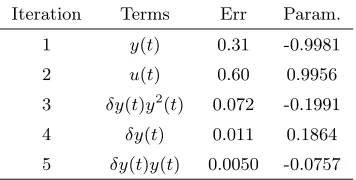
Iteration Terms Err Param. 1 y(t) 0.31 -0.9981 2 u(t) 0.60 0.9956 3 δy(t)y2
[image:7.595.75.253.75.165.2](t) 0.072 -0.1991 4 δy(t) 0.011 0.1864 5 δy(t)y(t) 0.0050 -0.0757 Table 2
Significant terms selected for theδ-domain non-linear model of the Van-der-Pol oscillator at a sampling frequency of 40Hz.
was an input delay) and then iteratively increasing the maximum order of non-linearitypup top= 5. The num-ber of terms selected in the FRO procedure was a super-set of 19 terms, which was pruned using the Bayesian Information Criterion (BIC) (Haber and Unbehauen, 1990).
The input-output order of theδ-domain model was de-tected asna = 2,nb= 0 and delayk= 0. The
identifica-tion of the difference equaidentifica-tion model was performed us-ing the usual backward shift operatorq−1, whereuq−1= u(t−1). The input-output order of theq-domain model was identified asna = 2,nb= 1 andk= 1. In the case
of both theδ- andq-domain models the maximum order of non-linearity was selected asp= 3.
The results of the model identification procedure are
shown for a sampling frequency of 40Hz, for the q
-domain model in table 1 and the δ-domain model in
table 2. These tables reveal the following points:
(1) The δ-domain model terms that are the
fast-sampling limit equivalents of the continuous-time model have dominated the structure selection and the corresponding parameter estimates of those terms are similar to the continuous-time values. (2) The FRO algorithm has attributed anErrof 1.00
to theq-domain termy(t−1), which implies that close to 100% of the data is described by that one term. This potential problem was initially implied by the analysis in section 4.2.
(3) The q-domain model contains significantly more terms than theδ-domain model, suggesting that the use of the δ-operator has lead to a more parsimo-nious structure.
5.3.1 Parameter Estimation
Figure 1 demonstrates that the information matrix that was inverted during least squares parameter estimation was ill-conditioned for theq-domain model, even at low sampling frequencies. This numerical problem was exac-erbated at higher sampling frequencies. In contrast the condition number of theδ-domain model was preserved across all sampling frequencies tested. This improvement in conditioning was notably present even at the slowest
0 50 100 150 200 250 300 350
102
104
106
108
1010
1012
1014
1016
Sampling Frequency (Hz)
Condition Number
δ−domain
[image:7.595.314.548.79.271.2]q−domain
Fig. 1. The condition number of the information matrix that is inverted during least squares parameter estimation.
sampling frequency which was 10Hz (5 times the excita-tion frequency bandwidth).
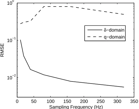
The parameters of theδ-domain model terms contained in (49) were found to converge towards the continuous-time values as the sampling rate was increased, as shown in figure 2. This suggests that the δ-domain parame-ters converge towards the continuous-time values, even whilst the relevant terms are contained as a subset of the full discrete-time model. The parameter estimates of theq-domain model terms contained in (50) were found to have some similarity to the expected values, as shown in figure 2, but not the same properties of convergence as the δ-domain model. This result shows that the lin-ear modelδ-operator property of parameter convergence can extend, in some cases, to that of non-linear system identification.
5.3.2 Structure Detection
The model terms expected to dominate the structure selection were the δequivalents of the continuous-time model and the correspondingq-domain model terms. It was found that the four expected δ-terms consistently dominated structure selection at all but the lowest sam-pling frequency (see table 3). In contrast the expected linear terms of theq-domain model dominated the struc-ture detection, but the expected non-linear terms ap-peared at inconsistent intervals (see table 4).
iden-Iteration Terms Err Param. 1 y(t−1) 1.00 2.0006
2 y(t−2) 5.19×10⁻⁶ -1.0006
3 u(t−1) 5.30×10⁻¹¹ 9.7390×10⁻⁶
4 y(t−1)u2(t−1) 2.03×10⁻¹³ 1.6993
×10−6
5 y(t−2)u2(t−1) 6.14×10⁻¹⁴ -1.7023×10⁻⁶
6 y3(t−2) 1.70×10⁻¹⁴ -0.5093
7 y3
(t−1) 4.20×10⁻¹⁴ 0.5080
8 y2(t−2) 3.98×10⁻¹⁴ 0.0023
9 y(t−1)y(t−2) 2.18×10⁻¹⁴ -0.0044
Table 1
Significant terms selected for theq-domain non-linear model of the Van-der-Pol oscillator at a sampling frequency of 40Hz.
Freq. (Hz) Model Terms
y(t−1) y(t−2) u(t−2) y3(t−2) y2(t−2)y(t−1)
10 1 2 3 5 7
20 1 2 3 5 7
40 1 2 3 6 10
80 1 2 3 6 10
160 1 2 3 9 10
[image:8.595.135.455.253.379.2] [image:8.595.323.529.410.535.2]320 1 2 3 9 10
Table 4
Iteration at which the relevantq-domain model term is selected in the FRO algorithm; with varying sample frequency.
0 50 100 150 200 250 300 350 10−2
10−1 100
Sampling Frequency (Hz)
RMSE
δ−domain q−domain
Fig. 2. Difference between continuous-time model param-eters and the estimated paramparam-eters corresponding to the model terms expected to be obtained in the fast-sampling limit for both theq- andδ-domain models.
tified non-linear model. This does not appear to be af-fected by increasing the sampling rate. This is a con-trasting result to that of parameter estimation, where the parameters do converge towards the continuous-time values as the sample rate increases.
Freq. (Hz) Model Terms
y(t) u(t) y2
(t)δy(t) δy(t)
10 1 2 3 6
20 1 2 3 4
40 1 2 3 4
80 1 2 3 4
160 1 2 3 4
320 1 2 3 4
Table 3
Iteration at which the relevantδ-domain model term is se-lected in the FRO algorithm; with varying sample frequency.
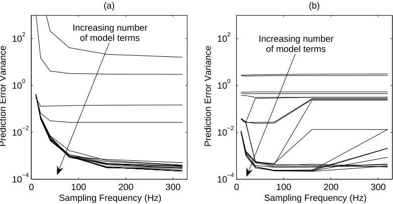
Figure 3(b) shows how the prediction error variance of theq-domain model has a tendency to increase at higher frequencies for a given number of model terms. This is in contrast to the δ-domain model; figure 3(a) shows that the error variance is decreased at higher sampling frequencies. This implies that the use of theδ-operator in non-linear system identification leads to more consistent performance across a range of sampling frequencies than theq-operator.
[image:8.595.48.283.419.603.2]0 100 200 300 10−4
10−2 100 102
Sampling Frequency (Hz)
Prediction Error Variance
(a)
0 100 200 300
10−4 10−2 100 102
Sampling Frequency (Hz)
Prediction Error Variance
(b)
Increasing number
of model terms Increasing number
[image:9.595.92.483.72.275.2]of model terms
Fig. 3. Prediction error variance at increasing sampling frequencies, where each line corresponds to a model with a given number of terms from 1 to 19 in the order selected by the FRO algorithm: (a)δ-domain and (b)q-domain.
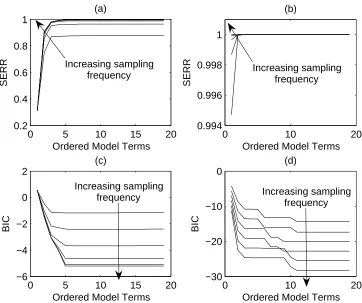
would have highErrand vice-versa. Therefore the sum of error reduction ratios (SERR) should be an indicator of model structure. Figure 4(a) indicates that there is a progressive usefulness in the selection of the first four terms in theδ-domain model, each of which have a di-rect correspondence to the continuous-time model (ex-cept in the case of the lowest sampling frequency). This progressive usefulness of model terms is not indicated in figure 4(b), for the q-domain model, where the SERR converges towards unity after the first term is selected. Note that this was to be expected from the analysis per-formed in section 4.2.
The BIC was used to truncate the ordered selection of model terms detected by the FRO algorithm. Figure 4(c) shows that the use of theδ-operator lead to the selec-tion of fewer terms at all sampling frequencies compared to theq-domain model, where the corresponding results are shown in figure 4(d). The use of theδ-operator in the test scenario presented here has consistently lead to a more parsimonious structure at fast and slow sampling frequencies; this implies that in general the use of the
δ-operator may lead to a more parsimonious description for certain model classes in non-linear system identifica-tion problems.
6 Conclusions
This investigation has shown the correspondence be-tween polynomial non-linear models described in theq -andδ-domains. This exact relationship implies the po-tential theoretical equivalence of the use of either op-erator in non-linear system identification. However, the practical application of non-linear modelling techniques (e.g. FRO structure selection) has highlighted the fact
that differences in identification (betweenqandδ) may arise, presumably resulting from numerical issues. Im-provements from using theδ-operator in the identifica-tion of a deterministic continuous-time non-linear sys-tem have been demonstrated, focusing on: (i) the con-vergence of the parameter estimates of the non-linear
δ-domain model to the continuous-time values (ii) the consistency of the detection procedure in terms of struc-tural linking to the continuous-time system and consis-tent selection of auxiliary model terms that contribute to an accurate system description at higher sampling fre-quencies, and (iii) the parsimonious model description.
7 Acknowledgements
The authors would like to acknowledge the anonymous reviewers and the Editor for System Parameter Estima-tion for their valuable comments.
References
Billings, S. A., Aguirre, L. A., 1995. Effects of the sam-pling time on the dynamics and identification of non-linear models. International Journal of Bifurcation and Chaos 5, 1541–1556.
Chadwick, M. A., Kadirkamanathan, V., Billings, S. A., 2006. Analysis of fast-sampled non-linear sys-tems: Generalised frequency response functions forδ -operator models. Signal Processing 86, 3246–3257. Chen, S., Billings, S. A., Luo, W., 1989. Orthogonal least
0 5 10 15 20 0.2
0.4 0.6 0.8 1
Ordered Model Terms
SERR
(a)
0 10 20
0.994 0.996 0.998 1
Ordered Model Terms
SERR
(b)
0 5 10 15 20
−6 −4 −2 0 2
Ordered Model Terms
BIC
(c)
0 10 20
−30 −20 −10 0
Ordered Model Terms
BIC
(d)
Increasing sampling frequency Increasing sampling
frequency Increasing sampling
frequency Increasing samplingfrequency
Fig. 4. (a) Sum of error reduction ratios of theδ-domain model. (b) Sum of error reduction ratios of theq-domain model. (c) Bayesian information criterion of model terms in theδ-domain model. (d) Bayesian information cost of model terms in the
q-domain model.
Fan, H., De, P., 2001. High speed adaptive signal pro-cessing using the delta operator. Digital Signal Pro-cessing 11, 3–34.
Fan, H., Soderstrom, T., Mossberg, M., Carlsson, B., Yuanjie, Z., 1999. Estimation of continuous-time AR process parameters from discrete-time data. IEEE Transactions on Signal Processing 47, 1232–1244. Goodwin, G. C., Middleton, R. H., Poor, H. V., 1992.
High-speed digital signal processing and control. Pro-ceedings of the IEEE 80, 240–259.
Haber, R., Unbehauen, H., 1990. Structure identifica-tion of nonlinear dynamic systems - a survey on in-put/output approaches. Automatica 26, 651–677. Kuznetsov, A., Bowyer, R., Clarke, D. W., 1999.
Esti-mation of multiple order models in theδ-domain. In-ternational Journal of Control 72, 629–642.
Larsson, E. K., Mossberg, M., Soderstrom, T., 2006. An overview of important practical aspects of continuous-time ARMA system identification. Circuits, Systems and Signal Processing 25 (1), 17–46.
Lauritsen, M. B., Rostgaard, M., Poulsen, N. K., 1997. GPC using delta-domain emulator-based approach. International Journal of Control 68, 219–232.
Leontaritis, I., Billings, S. A., 1985. Input-output para-metric models for non-linear systems Part 1:
deter-ministic nonlinear systems. International Journal of Control 2, 303–328.
Li, Q., Fan, H., 1997. On the properties of information matrices of delta-operator based adaptive signal pro-cessing algorithms. IEEE Trans. Signal Propro-cessing 45, 2454–2467.
Liu, G. P., Billings, S. A., Kadirkamanathan, V., 2000. Nonlinear system identification using wavelet net-works. International Journal of Systems Science 31, 1531 – 1541.
Middleton, R. H., Goodwin, G. C., 1986. Improved finite word length characteristics in digital control using the delta operator. IEEE Trans. Automatic Control 31, 1015–1021.
Middleton, R. H., Goodwin, G. C., 1990. Digital Control and Estimation: A Unified Approach. Prentice Hall, Englewood Cliffs, NJ.
Monaco, S., Normand-Cyrot, D., 1995. A unified repre-sentation for nonlinear discrete-time and sampled dy-namics. Journal of Mathematical Systems, Estimation and Control 5, 1–27.
[image:10.595.109.471.76.379.2]sig-nals and binary sequences with low autocorrelation. IEEE Transactions on Information Theory 16. Shim, K., Sawan, M. E., 2006. Singularly perturbed
uni-fied time systems with low sensitivity to model reduc-tion using delta operators. Internareduc-tional Journal of Systems Science 37 (4), 243–251.
Soderstrom, T., Fan, H., Carlsson, B., Bigi, S., 1997. Least squares parameter estimation of continuous-time ARX models from discrete-continuous-time data. IEEE Transactions on Automatic Control 42, 659–673. Suchomski, P., 2003. J-lossless and extended J-lossless
factorization approach for delta-domain H-infinity control. International Journal of Control 76, 794–809. Yuz, J. I., Goodwin, G. C., 2005. On sampled-data mod-els for nonlinear systems. IEEE Transactions on Au-tomatic Control 50.
A Proof of Lemma 3.1
Consider a single polynomial NARX model term χ(t) with non-linear order p, mapped to the δ-domain by substitution ofq= 1 +T δin (3),
p
Y
j=1 qnjφ
j(t) = p
Y
j=1
(1 +T δ)njφ
j(t) (A.1)
The terms arising from the RHS of this mapping can be be expressed as the ordered setMp,np,
Mp,np=
c0,1δ0φ1(t) × c0,2δ0φ2(t) ×. . .× c0,pδ0φp(t)
c1,1δ1φ1(t) × c0,2δ0φ2(t) ×. . .× c0,pδ0φp(t)
..
. ... ... ...
cn1,1δ
n1φ1(t)× c0,2δ0φ2(t) ×. . .× c0,pδ0φp(t) c0,1δ0φ1(t) × c1,2δ1φ2(t) ×. . .× c0,pδ0φp(t)
..
. ... ... ...
cn1,1δ
n1φ1(t)× c1
,2δ1φ2(t) ×. . .× c0,pδ0φp(t)
..
. ... ... ...
c0,1δ0φ1(t) × cn2,2δ
n2φ2(t) ×. . .× c0,pδ0φp(t)
..
. ... ... ...
cn1,1δ
n1φ1(t)× c
n2,2δ
n2φ2(t) ×. . .× c0
,pδ0φp(t)
c0,1δ0φ1(t) × c0,2δ0φ2(t) ×. . .× c1,pδ1φp(t)
c1,1δ1φ1(t) × c0,2δ0φ2(t) ×. . .× c1,pδ1φp(t)
..
. ... ... ...
cn1,1δ
n1φ1(t)× c0
,2δ0φ2(t) ×. . .× c1,pδ1φp(t)
..
. ... ... ...
..
. ... ... ...
c0,1δ0φ1(t) × cn2,2δ
n2φ2(t) ×. . .×c
np,pδ npφ
p(t)
..
. ... ... ...
cn1,1δ
n1φ1(t)× c
n2,2δ
n2φ2(t) ×. . .×c
np,pδ npφ
p(t)
(A.2)
The powersmk,j, ofδmk,jfromMp,npcan be defined for successive cross-product terms as (where the notation
mk,jindicates the power of thekthelement andjth
cross-product term),
mk,1 = mod (k−1, n1+ 1) mk,2 = mod
j
k−1
n1+1
k
, n2+ 1
mk,3 = mod
j
k−1 (n1+1)(n2+1)
k
, n3+ 1 ..
. ...
mk,p = mod
k−1
Qp−1
i=1ni+1
, np+ 1
(A.3)
be defined as
mk(t) = p
Y
j=1
cmk,j,jδ mk,jφ
j(t) (A.4)
The full mapping of aq-domain term to theδ-domain involves the summation of the rows of the setMp,npafter each row is scaled byTraised to the appropriate power. The appropriate power ofT corresponds to the sum of the powers ofδ in the rowk, ¯mk =Ppj=1mk,j. Hence
the mapping of a singleq-domain NARX termχ(t) is
p
Y
j=1 qnjφ
j(t) = r
X
k=1 Tm¯km
k(t) (A.5)
2
B Proof of Lemma 3.2
Consider the expression of a singleδ-domain polynomial NARX model term ψ(t) of order p mapped to the q -domain by substitution of (7) in (3)
p
Y
j=1 δnjφ
j(t) = p
Y
j=1
q−1
T
nj
φj(t) (B.1)
The terms arising from the expansion of (B.1) can be written as an ordered setM−
p,np similarly toMp,np, re-placing theδ-operator by the q-operator and the bino-mial coefficientscmk,j,j by c
−
mk,j,j and where each row ofM−
p,np is scaled by T
−m¯l,k. Hence the mapping of a singleδ-domain NARX termψ(t) to theq-domain is
p
Y
j=1 δnjφ
j(t) = r
X
k=1
Tm¯km−
k(t) (B.2)
wherem−
k(t) is thekthelement in the setM
−
p,np,
m−
k(t) = p
Y
j=1 c−
mk,j,jq mk,jφ
j(t). (B.3)
2
C Proof of Theorem 3.1
The mapping of thelth δ-domain toq-domain
polyno-mial NARX model term follows from the extension of Lemma 3.1,
pl
Y
j=1 qnl,jφ
l,j(t) = rl
X
k=1 Tm¯l,k
pl
Y
j=1
cl,ml,k,j,jδ ml,k,jφ
l,j(t).
(C.1)
where the application of Lemma 3.1 to the lth model
term leads to the definitions of (22), (23), (24) and (25). Hence the mapping of a full δ-domain model to theq -domain as defined in (21) follows immediately from the substitution of (C.1) in (4).
The preservation of the order of non-linearity when map-ping a single term of order pfrom the q- to δ-domain follows from the definition of the setMp,np, where the number of cross-product terms in each element, result-ing from the binomial expansion of (A.1), is exactlyp.
The set of term orders mk,j contained within the set
Mp,np is N = {0, . . . , n1, . . . ,0, . . . , np}. Correspond-ingly the set of term orders contained within the q -domain model termQp
j=1qnjφj(t) isNq ={n1, . . . , np},
i.enj ∈ Nq, forj= 1, . . . , p. Clearly,
max
k=1,...,r(N(k)) = maxj=1,...,p(Nq(j)) (C.2)
where the notation for a setN(k) indicates thekth
ele-ment of the set. By extension of (C.2) to the full model
composed ofwterms
max
l=1,...,w
max
k=1,...,rl
N(l)(k)
=
max
l=1,...,w
max
j=1,...,pl
N(l)
q (j)
(C.3)
which proves that the maximum time order of the model
terms is preserved when mapping between domains. 2
D Proof of Theorem 3.2
The mapping of the lthq-domain toδ-domain
polyno-mial NARX model term follows from the extension of Lemma 3.2,
pl
Y
j=1 δnl,jφ
l,j(t) = rl
X
k=1 T−m¯l,k
pl
Y
j=1 c−
l,ml,k,j,jq ml,k,jφ
l,j(t).
(D.1) where the application of Lemma 3.2 to the lth model
term leads to the definition of (27). Hence the mapping of a fullq-domain model to theδ-domain as defined in (26) follows immediately from the substitution of (D.1) in (10).
The preservation of the order of non-linearity when map-ping a single term of order pfrom the q- to δ-domain follows from the definition of the setM−
p,np, where the number of cross-product terms in each element, result-ing from the binomial expansion of (B.1), is exactlyp.
The set of term orders mk,j contained within the set
M−
p,np isN
− ={0, . . . , n1, . . . ,0, . . . , n
Correspond-ingly the set of term orders contained within the δ -domain model termQp
j=1δnjφj(t) isNδ ={n1, . . . , np},
, i.enj∈ Nδ, forj= 1, . . . , p. Clearly,
max
k=1,...,r N
−
(k)
= max
j=1,...,p(Nδ(j)) (D.2)
and by extension to the full model composed ofwterms
max
l=1,...,w
max
k=1,...,rl
N−(l)(k)=
max
l=1,...,w
max
j=1,...,pl
Nδ(l)(j)
(D.3)
which proves that the maximum time order of the model terms is preserved when mapping between domains.