Practical constraints on real time Bayesian filtering for NDE applications

Practical Constraints on Real time Bayesian Filtering

for NDE Applications

R. Summana, S. Piercea, G. Dobiea, J. Hensmanb, C. MacLeoda

a_{Department of Electronic and Electrical Engineering, University of Strathclyde, Glasgow,}

UK, G11XW.

b_{Department of Mechanical Engineering, Sheffield University, Sheffield, UK, S1 3JD}

Abstract

An experimental evaluation of Bayesian positional filtering algorithms applied to mobile robots for Non-Destructive Evaluation is presented using multiple positional sensing data - a real time, on-robot implementation of an Extended Kalman and Particle filter was used to control a robot performing representa-tive raster scanning of a sample. Both absolute and relarepresenta-tive positioning were employed - the absolute being an indoor acoustic GPS system that required careful calibration. The performance of the tracking algorithms are compared in terms of computational cost and the accuracy of trajectory estimates. It is demonstrated that for real time NDE scanning, the Extended Kalman Filter is a more sensible choice given the high computational overhead for the Particle filter.

Keywords: Robotics, Non-Destructive Evaluation, Bayesian Filtering

1. Introduction

Non-Destructive Evaluation (NDE) of engineering structures is an impor-tant and challenging task which can help to locate the presence and extent of structural defects before failure occurs. Regular NDE inspection of critical com-ponents can thus reduce costly outages, negative environmental impact as well as potential loss of life. A range of non-invasive NDE techniques are available including ultrasonic, visual, electromagnetic and radiography which are used to detect and characterise flaws in terms of their nature, size and position [1]. Through identification of anomalies, NDE can be used to replace only those components quantified to be defective and can thus contribute to the exten-sion of the operational life of the component/structure even perhaps beyond its designed lifetime.

Email addresses: [email protected](R. Summan),[email protected]

(S. Pierce),[email protected](G. Dobie),[email protected]

Industrial sectors for which NDE is of major importance include aerospace, nuclear and petrochemical extraction and processing. Such industries are a source of particular challenges, often presenting inspection sites located in inac-cessible locations or where environmental conditions are hazardous for human operators working at height, exposed to radioactivity, proximity to high temper-ature and/or pressure process plant. The financial impact of NDE inspections is also significant, arising from both the intrinsic inspection costs and the associ-ated cost of taking plant offline to conduct inspections [2]. Consequently in-situ automated inspection where feasible, is highly attractive, and potentially allows inspection of operational plant. The safety, environmental and financial bene-fits for automating NDE measurements are clear, and applicable across a broad range of NDE technology.

Automation is currently being addressed through deployment of sensor laden remotely controlled robotic devices, well established examples being pipeline inspection gauge (PIGS) systems [3] for internal pipe inspections or unmanned aerial vehicles (UAV) [4] for visual inspection. The use of such technology is very attractive in terms of safety, cost and the potential for minimal disruption to the inspection site especially if they allow plant operations to remain online. Robotic NDE inspection platforms are an active area of research, there are numerous examples in the literature proposing devices for a broad spread of application domains. A recent paper by Schempf et al [5] describes a robotic device to conduct inspections of natural gas distribution mains. The system is untethered and composed of interlocking modules allowing negotiation of pipe bends and utilizes a camera as the primary inspection sensor. Positioning is achieved through the use of encoders attached to the wheels of the modules and also through the counting of welds connecting pipe sections of known length. Shang et al [6] present a robotic system for inspecting non-ferrous aircraft wings and fuselages. The described robot is a large vehicle making use of suctions cups to adhere to the inspection surface. It has the capability of carrying a significant payload mass in the form of eddy current and thermographic sensors as well as a phased array probe and a solid coupled wheel probe. Fisher et al [7] developed a prototype system for surface inspection of gas tanks in ships making use of permanent magnets to adhere to the tank wall. The NDE sensor detected the leakage of injected helium from holes in the tank. White et al [8] developed a suction cup based system for inspection applications in the aerospace industry; a Kalman filter was used to fuse measurements from a Leica laser tracker and encoder data to determine the 6 d.o.f position of the robot.

Figure 1: RSA with air-coupled ultrasonic transducers attached. For a detailed description of the system architecture see [12]. Ultrasonic, magnetic flux leakage and eddy current sensors may be attached to the chassis in order to test the structure under investigation. Magnetic wheels are used to allow the robot to adhere to and negotiate 3D ferromagnetic structures.

Central to accomplishing the required degree of cooperating behaviour between multiple robots, is the is the accurate positioning of individual the RSA units.

Our requirement for integrating NDE measurements onto the robotic plat-forms presents a significant challenge to the positioning problem. For useful NDE images to be assembled from the RSA scanning, there are a number of physical influences on the measurement process that can considerably degrade the quality of the NDE images and thus their usefulness. For example in air-coupled ultrasonic imaging applications, the separation and orientation of the transducers to the sample is critical [13]. This is in addition to the basic degra-dation of image quality from the gross RSA positional uncertainty. For example it is not possible to assert defect presence or absence based upon comparison of expected time-of-flight (ToF) and measured ToF due to delays caused by error in location. As well as affecting the fundamental measurement principles used to identify defects, positioning is of importance to register NDE measurements from different sensors acquired from multiple scans conducted at different times. It important that the robot is able to return to the same structural location re-peatedly in order to monitor the time evolution of particular defects.

surfaces) and interaction with a priori unknown objects in the environment that may perturb the course of the robot [15]. These accumulated errors eventually lead to gross error between the true location and the encoder reported location. The effect is illustrated by simulation in Figure 2 showing the increase in error between the odometry reported path and actual path with trajectory length.

In order to reduce error in position the odometry must be supplemented with some other form of sensing. There are two main ways in which this sensory in-formation may be provided, firstly througha priori environmental information in the form of fixed known location beacons placed in the environment aiding the localisation of the robot. The second way is one in which no such external information is available and the robot must utilise purely its own onboard sen-sors to localise - the latter is known as Simultaneous Localisation and Mapping (SLAM) [14]. Both approaches although applicable in different cases make use of the same underlying filtering theory in order to combine sensor outputs. In the present work the output of the encoders are fused with an acoustic based GPS system for estimating the robot’s planar position [16].

Peralta-Cabezas et al [17] have investigated the first method in carrying out a comparison of ten Bayesian filters comprising of several variants of the Kalman and Particle filters as well hybrid filters that are composed of a combination of the two. Filtering was applied to a camera based tracking system and it was found that of all these filters the comparatively simple extended Kalman filter (EKF) and Particle filter (PF) perform best in terms of Mean Square Error (MSE) tracking error with respect to the true location of the robot. Tong and Barfoot [18] carried out a comparison of an EKF and sigma point Kalman filters for a 4-wheeled skid steer vehicle. The sigma point variant of the Kalman filter was found to be more robust and provided higher overall accuracy in comparison to the EKF. Bellotto and Hu examined the use of PF and Kalman filter based techniques in tracking people using a camera and laser range finder mounted on a robot.The authors showed that the Unscented Kalman filter performs as well as the PF at less computational cost.

In the current paper, comparative experimental results applicable to NDE measurements are presented for both EKF and PF tracking filters implemented on the on-board processing hardware of a single RSA unit. The structure of the paper is as follows, firstly the robotic hardware is presented followed by a statistical characterisation of the acoustic beacon positioning system. The filtering theory and implementation is then introduced followed by experimental evaluation of the performance, conclusions and future work.

2. Remote Sensing Agent (RSA)

−600 −400 −200 0 200 400 600 −600

−400 −200 0 200 400 600

Robot X Position (mm)

Robot Y Position (mm)

Figure 2: Typical raster path for NDE. Uncertainty in the robot’s position grows with time. The dashed line corresponds to the path reported by the odometry while the solid line pertains to the actual motion of the robot that may have resulted from wheel slippage on the corners of the path.

use of a Wi-Fi enabled 400 MHz Gumstix Connex [19] embedded processor to execute user defined instructions and process incoming sensory data. Each RSA individually constitutes an autonomous data acquisition and processing node. Detailed descriptions of the hardware have been previously published [12]. The integration of a flexible NDE measurement platform into the robot architecture is a clear differentiator for the Strathclyde RSA technology. Typically NDE sensors are not ”off the shelf” devices, but often complex instrumentation chal-lenges all of their own. The reader is referred to previous publications that discuss the actual development and operation of the NDE tools are detailed in [11]. The following section describes the kinematic model used by the filter algorithms.

2.1. Robot Model

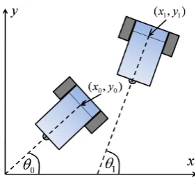
The location of a robot in 2D space is defined in Figure 3, it is determined by 3 variables - the (x, y) position of the drive axis midpoint andθ the angle of rotation with respect to the defined coordinate axes. The number of pulses pertaining to the left and right wheels available from the optical encoders, ∆r

and ∆l respectively, accrued in moving along the user specified line segment

allow prediction of the robot’s pose and is given by the following set of equations [15]:

xk=xk−1+



 rrcos(sin(θθkk−−11+ ∆+ ∆θθ)) ∆θ



 (1)

wherexk−1 is the pose of the robot at the previous time step, ∆θ=

c(∆r−∆l)

b

andr= c(∆r+∆l)

2 are the change in angle and the arc length traversed by the wheels between time stepskandk−1,cis the conversion factor between pulses and linear displacement and b is the distance between the drive wheels of the robot. It is the recursive nature of the odometry that causes the cumulative build of error evident in Figure 2: if at time stepk−1 the estimated position differs by an errorϵfrom the true state this is added to the subsequent estimate at time stepk.

3. Acoustic Beacon Location System

(a) (b)

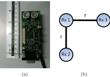
Figure 4: (a) A Cricket transceiver module. Inter-module distance is calculated from the time difference of arrival of simultaneous ultrasonic and RF emissions. (b)Arrangement of Cricket beacons. The RX’s are positioned on the corners of a quadrant of a circle with radius r.

of the ultrasonic pulse. The 1cm aperture and operating frequency produces a beamwidth at the -3dB point of ±26◦ with respect to the line perpendicular to the transducer face. The RF signal encodes the module identifier while the US serves to enable the TDoF calculation. The system compensates for the temperature perturbation of the speed of sound by using the mean of the temperatures measured at each module location.

Cricket may operate in 2 modes: the TX’s are fixed and the RX is mobile such that the TX’s must use a round-robin approach (in order to avoid signal interference amongst different modules) or the alternate mode where the TX is mobile and the RX’s are fixed resulting in round-robin updating of the robots. The former is preferred when multiple robots are in use allowing the platforms to simultaneously update their locations. Assuming three RX to TX distances have been acquired and given that the RX’s lie on a ring with radius r the location of the TX is calculated by trilateration [16] as follows:

  xytxtx

ztx

 =

 

1 2r(d

2

1−d22+r2) 1

2r(d

2

1−d23+r2)

±√(d2

1−x2−y2) 

 (2)

whered1,d2andd3are 3 RX - TX distances output from Cricket. The distances d1,d2andd3can be obtained very easily given a (x, y) robot location as follows:

db=

√

(x−xb)2+ (y−yb)2+z2b (3)

where (xb, yb, zb) are the beacon locations forb∈ {1,2,3}. The following section

3.1. Spatial accuracy and correction of Cricket Measurements

The accuracy of the distance measurements returned by a Cricket module was experimentally measured in one and two dimensions. The 1D experiment consisted of holding a TX static while a RX unit was moved in increments of 20mmalong a measurement rail with 1mmresolution from 0−2000mm with 15 individual distance measurements being acquired at each increment. The range of 2000mm was chosen because this fits within the inspection area used in the experimental evaluation section. Plotting the mean Cricket measured distance against the true distance (the line y = x) yields the graph shown Figure 5 clearly showing an error in gradient and offset. This was due to the clock frequency on the Cricket modules running at a frequency of 7.3728MHz rather than 8MHz assumed in the Cricket software. The distance measurements corrected to account for this error.

0 500 1000 1500 2000

0 200 400 600 800 1000 1200 1400 1600 1800 2000

True range (mm)

Measured range (mm)

True

Cricket

Figure 5: Cricket measured distance vs True distance over a distance of 0 to 2000mm. Cricket distance is calculated as the mean point at each measurement location where the points used to calculate the mean values are shown as dots.

The positional accuracy of the Cricket system in two dimensions was mea-sured through the acquisition of 300 measurements at each intersection point of a 7x7 grid with divisions of size 100mm x 100mm with and a resolution of 0.5mm; finer dimensions than considered in [16].

−400 −300 −200 −100 0 100 200 300 400 −400

−300 −200 −100 0 100 200 300 400

Beacon X Position (mm)

Beacon Y Position (mm)

Figure 6: Cricket uncertainty in the XY plane. The crossed points represent raw measurements with the 1D correction applied while starred points result from the spatial correction and the dots are the true location of the TX

consisted of measuring with Cricket known corner points of the rectangular 600mmx 500mminspection area used in the experiments to form the following matrix:

A=

(

BRx T Lx

BRy T Ly

)₋1

(4)

where (BRx, BRy), (T Lx, T Ly) were the bottom right and top left corners of

the inspection area respectively. A Cricket measurement p_m = (x, y) then undergoes a transform under A

P′=APm (5)

yielding the pointP′ = (x′, y′) which is subsequently passed through another transformation to form the calibrated pointPcalib as follows:

Pcalib= (

x

1−(_yy_′)(1−x′))(

y 1−(x

x′)(1−y′)

) (6)

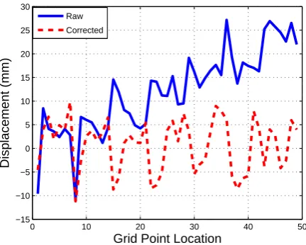
0 10 20 30 40 50 −15

−10 −5 0 5 10 15 20 25 30

Grid Point Location

Displacement (mm)

Raw

Corrected

Figure 7: Error in the calibrated (dashed line) and uncalibrated cases (solid line)

distribution of noise. The uncertainty of the distance readings returned from Cricket was evaluated after the spatial realignment and it was found that the histogram of distances pertaining to each measurement location was a function of the grid position and in the worst case followed a zero mean Gaussian density with a variance of 23mm2

4. Recursive Bayesian Filtering

The recursive Bayesian filter provides a probabilistic framework to fuse mul-tiple measurements in order to better estimate some variable of interest and in doing so it takes account of the uncertainties associated with the measurement sources [20]. A model of the system orprocess whose outputxis to be tracked is used to predict the distribution overx at time instantk−1 using equation 7 in the absence of any measurement of the process. This prediction is sub-sequently updated in light of a measurement z that has arrived at time step k using Equation 8 to produce a posterior distribution overx. Because these equations are in general computationally intractable this filter is not realisable in practice therefore approximations are used: the Kalman and Particle filters described in the following sections are such approximations.

p(xk|Zk−1) =

∫

p(xk|xk−1)p(xk−1|Zk−1)dxk−1 (7)

p(xk|Zk) =

p(zk|xk)p(xk|Zk−1)

p(zk|Zk−1)

4.1. Extended Kalman Filter (EKF)

The Extended Kalman filter [21], a state-space formulation, assumes zero mean Gaussian distributed noise sources. It predicts and propagates forward in time the covariance associated with the current estimate of pose. The state estimate is represented as a 3-vectorxwhose components comprise the variables defined in Figure 3, this estimate has an associated uncertainty which is encoded in the covariance matrix Σ these quantities are shown in Equation 9:

¯

x=

 xy

θ  ,Σ =

  σ

2

x σxσy σxσθ

σyσx σy2 σyσθ

σθσx σθσy σ2θ



 (9)

The state vector was modelled, using Equation 1, as a non-linear function, f, of the previous state and odometry:

xk=f(xk₋1,uk) +ϵk (10)

where xk is the pose of the robot, uk is the odometry measurement and ϵk

is a zero mean Gaussian noise source with covariance matrix R. A beacon measurement is modelled as follows:

zk=h(xk−1) +δk (11)

wherehis the function of Equation 3, zk= [d1, d2, d3]T is a measurement con-sisting of 3 beacons distances andδk is a zero mean Gaussian noise source with

covariance matrixQ. The entries ofQcontain the experimentally derived vari-ances in distance estimate from the acoustic location system. The Kalman filter implements the prediction-update cycle as follows. Using the process model and odometry only the prediction step estimates through Equations 11 and 12 the state and uncertainty associated with this state yielding ¯xkand ¯Σk respectively.

These predicted quantities are subsequently adjusted in light of the acoustic po-sitional measurement by Equations 14 and 15 giving, xk and Σk respectively.

The influence of the acoustic measurement is controlled by the Kalman gain matrixKk computed by Equation 13. The sequence of equations is as follows:

¯

xk=f(uk,xk−1) (12)

¯

Σk=GkΣk−1GTk +R (13)

Kk = ¯ΣkHkT(HkΣ¯kHkT +Q)−1 (14)

xk =x¯k+Kk(zk−h(x¯k)) (15)

Σk= (I−KkHk) ¯Σk (16)

where Gk, Hk are Jacobian matrices - required to propagate the state

uncer-tainty - of the state and measurement equations differentiated with respect to the state _∂x∂f

k−1,

∂h

Gk =



10 01 rrcos(sin(θθkk−−11+ ∆+ ∆θθ))−−rrsin(cos(θθkk−−1)1)

0 0 1



 (17)

Hk=

 (x

b1−_x¯

k−1)/d1 (yb1−y¯k−1)/d1 0 (xb2−_x¯

k−1)/d2 (yb2−y¯k−1)/d2 0 (xb3−_x¯

k₋1)/d3 (yb3−y¯k₋1)/d3 0 

 (18)

wheredb=

√

(¯x−xb)2+ (¯y−yb)2forb∈ {1,2,3}.

4.2. Particle Filter

Particle filtering is a sequential Monte Carlo technique that uses a sample based representation of the probability distribution associated with robot pose. It does not make the Gaussian noise assumption of the EKF and so maybe considered as being more generic than the EKF. This distribution is represented as a collection of pose, weight pairs of the form {xi_k, w_ki}N_i=1, where N is the number of samples taken to approximate the true distribution,xi_kis theith pose sample andw_ki is its associated weight which is proportional to the probability of being the true pose of the robot. The probability distribution over pose is then represented as a weighted shifted sum of delta functions as follows:

p(xk|Zk)≈

N

∑

i=1

wi_kδ(xk−xik) (19)

where Zk is the set of all measurements received up until time k. The PF

estimate of robot pose is simply the expected value of this distribution calculated by:

xk =

N

∑

i=1

xi_kw_ki (20)

Sampling from the posterior (19) is difficult because in general an analytic representation is not readily available [22], therefore, another simpler distribu-tion termed the proposal or importance distribudistribu-tion that shares the same sup-port as the posterior is used instead. The conventional choice is the transitional distribution [23]p(xk|xk−1) i.e. the robot motion model of Equation 1. The prediction step of the predict-update cycle is implemented through sampling from this distribution.

The integration of a measurement into the PF is implemented through com-putation of the sample weights. The normalised weights (such that∑N_i=1wi

k =

1) associated with the particles are calculated using Equation 3 implemented in the likelihood function as follows:

w_ki =w_ki₋₁p(zk|x

i k)

∑N i=1wik

in which, assuming independent and identically distributed samples,p(zk|xik)

is given by:

p(zk|xik) =

R∏=3

b

1 √

2πσ2

beacon

e(

(√(xi−xb)2 +(yi−yb)2 +z2

b−db)2

−2σ2 beacon

)

(22)

where (xi, yi) is the predicted location of the robot by theith particle,σbeacon2 is

the variance of the TX to RX distance approximated by a Gaussian distribution with the remaining variables as defined in Equation 3. The likelihood function in effect assigns more weight to those particles closer to an incoming beacon measurement, where the size of the weight is a function of the variance of the distance measurements.

A key step in this algorithm is that of resampling the particles which involves discarding particles with low weight and replicating those particles with higher weights due to their higher probability of being the true location of the robot. Resampling may be invoked every time the PF runs or when the number of effective particlesNEF F falls below a threshold calculated as follows:

NEF F =

1 ∑N

i=1(w

i k)2

(23)

There are numerous resampling algorithms that maybe used, it was found that stratified resampling [23] applied whenNEF F dropped below 80% produced the

best results during the experimental evaluation.

5. Experimental Evaluation of EKF vs PF

Efficient C++ implementations of the EKF and PF were written for exe-cution on-board the RSA. To comply with best practice, the UMBMark [24] procedure was carried out to fine tune the wheel base and wheel diameters to ensure optimal odometry estimation. Ground truth was measured using a commercial state-of-the-art photogrammetry based dynamic motion tracking system, Vicon MX. Using a calibrated 6 camera T160 system, the robot pose (translation and orientation) could be tracked with sub-millimetre accuracy. The following sections describe the method used to align the coordinate frames of the different tracking systems used in the experiment followed by the evalu-ation of the implemented algorithms on real world data representative of NDE scanning.

5.1. Coordinate Frame Alignment

The modules were then aligned using the Vicon reported locations. Alignment between the Cricket and Vicon coordinate frames was achieved through the sin-gular value decomposition (SVD) of the correlation matrix resulting from the product of corresponding point pairs measured by both systems following the method of N¨uchter [25]. The systems were configured to track the same physical point on the robot acquiring 300 measurements at 5 grid locations yielding the point setsp_v andp_c for the Vicon and Cricket systems respectively solving the correspondence problem by default. Equations 24 and 25 define the correlation matrix and SVD procedure that allowed the relative rotation and translation, Randt to be recovered respectively

H =

N

∑

i=1

p′_viTp′_ci= 

SSxxyx SSxyyy SSxzyz

Szx Szy Szz



 (24)

H=UΛVT, R=V UT, t=p¯c−Rp¯v (25)

wherep′v andp′care the point sets with their respective means removed andp¯c andp¯vare the point set centroids. The average displacement error between the transformed Vicon points and the raw Cricket measurements wasϵ=−3.7mm. This was the best error that could be achieved in practice and manifests as an offset in the errors calculated in the following section.

5.2. Raster Scan Experiment

To simulate a typical course employed in a real NDE scan a robot was instructed to execute a raster scan consisting of 600mm horizontal sweeps and 100mmvertical sweeps contained in the rectangle of dimension 600mmx 500mm starting with the pose p_start = [300mm,−300mm,180◦]T _{in the plane. This}

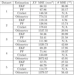
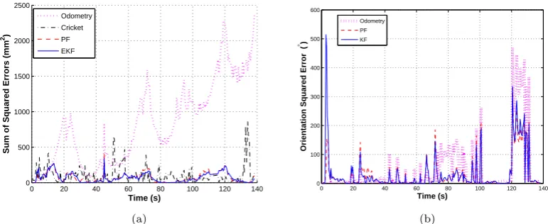
scan was repeated multiple times to generate 5 different datasets for analysis. The trajectory estimates from all estimation sources for dataset 1 are shown in the graph of Figure 8a. The EKF and PF (using 200 particles) curves have a stronger correlation with the Vicon curve than odometry which becomes in-creasingly erroneous. The estimation squared errors of each source with respect to ground truth is shown in Figure 9a while the numerical MSE errors are tab-ulated in Table 1. It is clear from the graphs that the error in odometry grows with path length, its oscillatory behaviour being due to the robot turning back to ground truth on corner rotations thus reducing the accumulating error. The filter estimates are essentially a smoothed version of the Cricket data where the odometry fulfils the smoothing function. It is clear from Table 1 that the error of both the PF and EKF is less than that of the positional sources used in iso-lation. Inspection of Table 1 confirms the reduction of positional error enabled through filtering for different datasets.

executed offline on a PC. From this result it maybe concluded that the system is sufficiently linear within the system time-step defined by the odometry such that the potential gains offered by the PF are cancelled out. This conclusion was tested by considering the scenario in which the odometry arrives at a slower rate. The encoder data was decimated by a factor of 10 in effect simulating a larger time-step, 10 times greater than the raw data. The resultingN vs error plot is shown in Figure 11 where the PF curve now intersects at approximately 50 particles and subsequently saturates below the EKF curve where each PF point is again 5 runs averaged. The larger time-step means that the EKF has to linearise a more non-linear region of the state-space which gives rise to greater linearisation error and subsequently higher MSE. The saturation of the PF error to the level of the EKF in Figure 10 suggests that the EKF is Bayes optimal as when N becomes large the PF becomes Bayes optimal. It maybe said from Figure 11 that the PF is more efficient in the sense that it produces an error in the decimated-data case comparable to the case processing the raw data.

The computational cost of running the filters onboard the robot is an impor-tant factor in practice since the robot has other processing tasks running during operation. The EKF is less of a computational burden in comparison to the PF in which execution time is a function of the number of particlesN. Measuring execution time resulting from running a single predict-update cycle for each filter while varying N, yields Figure 12. The curve is valid for the particular implementation on the specific hardware being used but gives an idea of the trend that would be true given another implementation/hardware combination. The PF curve displays a linear growth with N, reaching a value of approxi-mately 17ms when using 3000 particles whereas the EKF approximately stays constant with a value of 0.04ms. The EKF is more suited to realtime operation particularly when more functions are added to extend the robots capabilities.

6. Conclusion

NDE plays a critical role in industry with regard to pre-empting component failure and thus averting economic and human cost. This paper focused upon methods to accurately localise a (purpose built) robotic vehicle proposed to operate in a multi-robot NDE scanning system. The vehicle receives noisy positional updates from onboard wheel encoders and an external acoustic based GPS system at 100Hz and 3Hz respectively. The former is a relative system that is subject to drift like all such methods of estimation, while the latter provides absolute updates too infrequently for practical use. The use of EKF and PF Bayesian filters was investigated for combining the available positional estimates and an experimental comparison of the performance of these filters was performed.

Dataset Estimation XY MSE (mm2_{) θMSE (}◦2₎

1

EKF 66.53 36.06

PF 67.86 33.17

Cricket 146.58 N/A

Odometry 774.51 51.07

2

EKF 119.18 8.76

PF 138.94 15.74

Cricket 178.61 N/A

Odometry 1537.55 20.94

3

EKF 50.36 20.99

PF 53.41 21.58

Cricket 111.90 N/A

Odometry 1320.73 42.68

4

EKF 69.29 17.95

PF 71.84 19.37

Cricket 133.69 N/A

Odometry 2072.62 45.91

5

EKF 57.75 27.55

PF 60.79 27.40

Cricket 114.77 N/A

Odometry 1379.57 56.43

Table 1: Pose error for each estimation source with respect to ground truth for each dataset

−400 −300 −200 −100 0 100 200 300 400

−400 −300 −200 −100 0 100 200 300

Robot X Position(mm)

Robot Y Position(mm)

ODOM EKF PF VICON CRICKET

(a)

0 20 40 60 80 100 120 140 −50

0 50 100 150 200 250

Time (s)

Robot Orientation (

°)

Vicon Odometry PF KF

(b)

0 20 40 60 80 100 120 140 0

500 1000 1500 2000 2500

Time (s)

Sum of Squared Errors (mm

2)

Odometry

Cricket PF

EKF

(a)

0 20 40 60 80 100 120 140 0

100 200 300 400 500 600

Time (s)

Orientation Squared Error (

°)

Odometry PF KF

(b)

Figure 9: (a) Error in (x, y) position of trajectory estimates with respect to Vicon (b) Error of robot orientation

linear within the system time step (dictated by the encoders) that the potential benefits of the PF do not become apparent. Indeed it also shown that if the rate of the encoder data is reduced the EKF estimation error increases as a consequence of larger linearisation error. Within the constraints of the described system, the conclusion that can be drawn from this experiment is that there is no benefit in using the PF. This, however, is not true in general and shows that choice of filtering technique is dependent upon both the system setup and the models employed in the algorithms. A practical aspect of importance for resource limited systems such as the presented system is the computational cost of algorithms running onboard. An attractive benefit of the EKF it is the ability to compute the update in a fixed time period while the cost associated with the PF is proportional to the number of particles used of which the optimal number is not always clear.

Future work will incorporate multiple NDE scan results from a structural inspection using similar filtering algorithms to enable data fusion.

Acknowledgement

This research received funding from the Engineering and Physical Sciences Research Council (EPSRC) and forms part of the core research program within the Research Centre for Non-Destructive Testing (RCNDE), in the UK.

References

101 102 103 0.4

0.6 0.8 1 1.2 1.4 1.6 1.8 2 2.2

x 104

N

MSE (mm

2 )

PF EKF

Figure 10: PF saturates to the level of the EKF in processing raw data. Error bars are plotted for each PF point showing range of values used to calculate the mean point.

[2] P. Cawley, “Non-destructive testing-current capabilities and future direc-tions,” Proceedings of the Institution of Mechanical Engineers, Part L: Journal of Materials: Design and Applications, vol. 215, no. 4, pp. 213–223, 2001.

[3] “Pipeline inspection technologies demonstration report,” tech. rep., US De-partment of Transportation Pipeline and Hazardous Materials Safety Ad-ministration., March 2006.

[4] D. L. von Berg, S. A. Anderson, A. Bird, N. Holt, M. Kruer, T. J. Walls, and M. L. Wilson, “Multi-Sensor Airborne Imagery Collection and Processing Onboard Small Unmanned Systems,” in AIRBORNE INTELLIGENCE, SURVEILLANCE, RECONNAISSANCE (ISR) SYSTEMS AND APPLI-CATIONS VII (Henry, DJ, ed.), vol. 7668 of Proceedings of SPIE-The International Society for Optical Engineering, SPIE, SPIE-INT SOC OP-TICAL ENGINEERING, 2010.

[5] H. Schempf, E. Mutschler, A. Gavaert, G. Skoptsov, and W. Crowley, “Vi-sual and nondestructive evaluation inspection of live gas mains using the ExplorerTM family of pipe robots,”Journal of Field Robotics, vol. 27, no. 3, pp. 217–249, 2010.

[6] J. Shang, T. Sattar, S. Chen, and B. Bridge, “Design of a climbing robot for inspecting aircraft wings and fuselage,”Industrial Robot: An International Journal, vol. 34, no. 6, pp. 495–502, 2007.

101 102 103 0.6

0.8 1 1.2 1.4 1.6 1.8 2 2.2 2.4x 10

4

N

MSE (mm

2 )

PF EKF

Figure 11: PF falls below the EKF line when data is decimated. Error bars are plotted for each PF point showing range of values used to calculate the mean point.

wheels,” in Intelligent Robots and Systems, 2007. IROS 2007. IEEE/RSJ International Conference on, pp. 1216–1221, IEEE, 2007.

[8] T. White, R. Alexander, G. Callow, A. Cooke, S. Harris, and J. Sargent, “A mobile climbing robot for high precision manufacture and inspection of aerostructures,” The International Journal of Robotics Research, vol. 24, no. 7, p. 589, 2005.

[9] M. Friedrich, L. Gatzoulis, G. Hayward, and W. Galbraith, “Small in-spection vehicles for non-destructive testing applications,” Climbing and Walking Robots, pp. 927–934, 2006.

[10] M. Friedrich, G. Dobie, C. Chan, S. Pierce, W. Galbraith, S. Marshall, and G. Hayward, “Miniature Mobile Sensor Platforms for Condition Monitoring of Structures,”IEEE SENSORS JOURNAL, vol. 9, no. 11, p. 1439, 2009.

[11] G. Dobie, A. Spencer, S. Pierce, W. Galbraith, K. Worden, and G. Hay-ward, “Simulation and Implementation of Ultrasonic Remote Sensing Agents for Reconfigurable NDE Scanning,” in AIP Conference Proceed-ings, vol. 1096, p. 990, 2009.

[12] G. Dobie, W. Galbraith, M. Friedrich, S. Pierce, and G. Hayward, “Robotic Based Reconfigurable Lamb Wave Scanner for Non-Destructive Evalua-tion,” inIEEE Ultrasonics Symposium, 2007, pp. 1213–1216, 2007.

0 500 1000 1500 2000 2500 3000 0

2 4 6 8 10 12 14 16 18

N

Execution Time (ms)

PF

EKF

Figure 12: On-board execution time for a single predict-update cycle. The spikes at N = 2160 and N = 2410 result from increased CPU activity due to other processes running concurrently

[14] H. Durrant-Whyte and T. Bailey, “Simultaneous localisation and mapping (SLAM): Part I the essential algorithms,” Robotics and Automation Mag-azine, vol. 13, no. 2, pp. 99–110, 2006.

[15] J. Borenstein, H. Everett, and L. Feng, “Where am I? Sensors and methods for mobile robot positioning,” University of Michigan, vol. 119, p. 120, 1996.

[16] N. Priyantha, The cricket indoor location system. PhD thesis, Mas-sachusetts Institute of Technology, 2005.

[17] J. Peralta-Cabezas, M. Torres-Torriti, and M. Guarini-Hermann, “A com-parison of Bayesian prediction techniques for mobile robot trajectory track-ing,”Robotica, vol. 26, no. 05, pp. 571–585, 2008.

[18] C. Tong and T. Barfoot, “A Comparison of the EKF, SPKF, and the Bayes Filter for Landmark-Based Localization,” in Computer and Robot Vision (CRV), 2010 Canadian Conference on, pp. 199–206, IEEE, 2010.

[19] “Gumstix inc..” http://www.gumstix.com/, Accessed June 2011.

[20] S. Thrun, W. Burgard, and D. Fox,Probabilistic robotics. MIT Press, 2008.

[21] R. Kalmanet al., “A new approach to linear filtering and prediction prob-lems,”Journal of basic Engineering, vol. 82, no. 1, pp. 35–45, 1960.

[23] B. Ristic, S. Arulampalam, and N. Gordon, “Beyond the Kalman filter,” IEEE Aerospace and Electronics Systems Magazine, vol. 19, no. 7, pp. 37– 38, 2004.

[24] J. Borenstein and L. Feng, “UMBmark: A benchmark test for measuring odometry errors in mobile robots,” Ann Arbor, vol. 1001, pp. 48109–2110.