Application of the functional renormalization group method to classical free energy models
Leo Lue1,a)
Department of Chemical and Process Engineering, University of Strathclyde James Weir Building, 75 Montrose Street, Glasgow G1 1XJ,
United Kingdom
(Dated: 31 May 2015)
A simple functional renormalization group method is presented to correct the behavior of
classical free energy models near the critical point. This approach is applied to the
Soave-Redlich-Kwong equation of state to illustrate its ability to better reproduce the phase behavior
of simple fluids and to understand the influence of its parameters on the shape of the
vapor-liquid phase diagram. The method is then extended to account for the correlations induced
by intramolecular bonds. It is then applied to a first order thermodynamic perturbation theory
for chain fluids to examine fluids composed of linearly bonded Lennard-Jones atoms. Unlike
previous approaches for applying renormalization group corrections to chain fluids, this is
able to accurately reproduce the critical point without predicting an overly flat liquid-vapor
coexistence region.
INTRODUCTION
Large-scale density fluctuations lead to universal scaling behavior of the free energy of a fluid
near the critical point. These take the form of non-analytic behavior of the free energy, which are not
present in the classical free energy models typically used by engineers to describe the thermodynamic
behavior of fluids. As a consequence, there can be significant deviations of the predictions of these
free energy models from experimentally observed results.
Much of the early work in describing this non-classical phenomena originally focused only on
states near the critical region. Phenomenological approaches have been used to combine the results of
this work with classical thermodynamic models in order to construct a free energy model that has the
correct scaling behavior in the critical regime and the classical behavior of the original model away
from the critical point. This crossover approach has been applied to several classical free energy
models, including cubic equations of state1–3, the perturbation theory for square-well fluids4, and
statistical associated fluid theory (SAFT)5,6.
Another method which gained popularity is the phase-space cell approximation, which was
orig-inally developed by Wilson7,8 and extended to describe the behavior of simple fluids by White and
coworkers9–11. This approach was later modified12, including mixtures13, and cubic equations of
state14. This method is relatively easy to apply to any free energy model.
There have been several attempts in recent years to apply the phase-space cell method to fluids
containing chain molecules15–17. Typically, these formulations are based on the SAFT or related
equations of state. These types of theories account for the connectivity of the molecules only in a
local fashion. When the phase-space cell method has been applied to long chain systems, it has been
observed that the predicted vapor-liquid coexistence curve becomes spuriously broad and flat15–17.
This artifact is due, in part, to the neglect of density correlations that arise from the intramolecular
bonding in the system.
It has been recognized that forms of the free energy of chain molecules that only depend on the
polymer concentration through the monomer packing fraction lead to the wrong scaling behavior of
the second virial coefficient with polymer molecular weight18. These include SAFT and the
Flory-Huggins models. Attempts have been made to combine the renormalization group for polymers with
the SAFT equation for linear19 and star polymers20, however, these were limited to the good solvent
regime and do not apply to phase separating systems.
A rigorous, molecularly based approach to applying the renormalization group method to classical
fluids is the hierarchical reference theory (HRT)21–23. This method accounts for the influence of long
range density fluctuations by examining the changes in the free energy of a fluid with changes in the
theory, a direct connection is made with the underlying molecular properties of the system. HRT
is able to accurately describe the crossover from the universal behavior of the free energy near the
critical point to its more specific, molecularly dependent properties outside the critical region. This
method has been successful in describing the properties of simple fluids21,22and mixtures24. The main
shortcomings of this approach are its complexity and computational requirements.
Still another approach is the functional renormalization group (FRG) method25, which has found
many applications in the areas of quantum field theory and condensed matter physics. Recently, a
close connection between FRG and hierarchical reference theory has been found26.
Ionescu and co-workers have formulated27 a sharp cut-off version of HRT and demonstrated its
application to the φ4 model. This functional renormalization approach offers a simple method for
providing critical corrections to classical free energy models. In this work, we demonstrate its
appli-cation. In addition, we provide a slight generalization of this method to account for the correlations
in chain molecules.
The remainder of this paper is organized as follows. In the next section, we discuss the functional
renormalization method and present a rough derivation for its application to free energy models for
classical fluids. Afterward we apply this functional renormalization method to a cubic equation of
state. We then discuss the issue of critical corrections for chain molecules, and then generalize the
method to apply to fluid composed of extended molecules. Finally, this method is used to describe
the phase behavior of a Lennard-Jones chain fluid.
FUNCTIONAL RENORMALIZATION GROUP METHOD
In this section, the basic ideas behind the functional renormalization group method and its
applica-tion to classical fluids are discussed. We consider a simple fluid that interacts with a pairwise additive
potentialu, which can be divided into a
u(r) =uref(r) +ul(r) (1)
where ul is the attractive portion of the interaction potential between molecules in the system, and
uref is the shorter ranged repulsive portion of the interaction potential. Typically, we assume that the
free energy functionalFref[ρ](whereρ(r)is some density profile) of a fluid that interacts only with
the reference portion of the potentialuref is known.
The grand partition function Ξ of the classical molecular system can be formally written as a
functional integral12
Ξ[γ] =
Z
Dρ(·) exp
( Z
drγ(r)ρ(r)−β 2
Z
drdr0ρ(r)ul(|r−r0|)ρ(r0)−Fref[ρ]
)
whereβ= (kBT)−1withT being the absolute temperature of the system andkBbeing the Boltzmann
constant, andγ is an applied external field. The functional integral overρ represents the summation
of the exponential term evaluated at all permissible “shapes” of the density profile in the system This
expression is formally exact, however, in practice it is not possible to evaluate without making further
approximations.
One method to approximate the functional integral is to completely neglect the fluctuations in
the density profile, and to simply take the largest value of the integrand. This leads directly to the
mean-field approximation28:
F[ρ]≈Fref[ρ] +
β 2
Z
drdr0ρ(r)ul(|r−r0|)ρ(r0). (3)
whereF is the free energy function of the fluid with the pairwise interaction potentialu =uref +ul.
This approximation is fairly good away from the critical point; however, near the critical regime,
density fluctuations make a significant contribution to the properties of the system, and the mean-field
approximation becomes increasingly poor.
Rather than attempting to evaluate the entire contribution of the density fluctuations at once,
an-other approach is to try to sequentially integrate the density fluctuations of increasing wavelength in
order to obtain a series of approximations to the free energy. The rationale behind this is that it may
be easier to approximate the change of the free energy due to a limited set of fluctuations. This is the
idea behind the renormalization group method.
The starting point of this method is to assume that we know the free energy functionalFΛ[ρ], which
is the free energy functional that includes fluctuations on length scales less than2πΛ−1 and neglects those with a lower wavenumber. Note that a good approximation for FΛ[ρ] is easier to obtain than
F[ρ], because small wavelength fluctuations (i.e. fluctuations with wavenumbers greater than2π/σ, whereσ is the size of a molecule) are usually strongly suppressed by excluded volume interactions.
We assume that a good approximation for the functionalFΛis available, for some value ofΛ∼2π/σ.
The grand partition function given in Eq. (2) can be rewritten as12
Ξ[γ] =
Z
Λ
Dρ(·) exp
( Z
drγ(r)ρ(r)− β 2
Z
drdr0ρ(r)ul(|r−r0|)ρ(r0)−FΛ[ρ]
)
(4)
where the functional integral over the density is now restricted to fluctuations with wavenumbers less
thanΛ.
To implement the renormalization group method, we construct a series of approximations to the
grand partition functionΞQ, where only density fluctuations of wavenumber greater thanQand less
thanΛare integrated over. IfQ≥Λ, then the free energy functional associated withΞQwill be equal
to
FΛ[ρ] +
β 2
Z
as all density fluctuations will be suppressed, and the mean-field approximation will be valid.
The grand partition function of a system in the absence of density fluctuations with a wave number
belowQcan in principle be evaluated by adding an additional two-body interactionRQto the system
which will suppress long range fluctuations:
ΞQ[γ] =
Z
Λ
Dρ(·) exp
( Z
drγ(r)ρ(r)− β 2
Z
drdr0ρ(r)ul(r,r0)ρ(r0)
−1 2
Z
drdr0ρ(r)RQ(|r−r0|)ρ(r0)−FΛ[ρ]
) (5)
The precise form of the cut-off functionRQis arbitrary, however, it must satisfy some key requirements23.
First, its Fourier transformRˆQ(q)must be a monotonic function ofqand vanish rapidly asqbecomes
very large. This ensures that it does not influence the functional integration over density profiles with
a short wavelength. In addition, it should become large as q ≤ Q; this is the mechanism by which
it suppresses the contribution of large wavelength fluctuations. In this work, we use the “optimized”
cut-off function suggested by Litim29,30
ˆ
RQ(q) =K(Q2−q2)Θ(Q−q) (6)
whereΘis the Heaviside step function, andKis an arbitrary constant.
We do not want to directly evaluate the functional integral in Eq. (5). Rather, we want to know
how the free energy changes with respect to changes in Q, given by changes in RQ which can be
interpreted as changes in the interaction potential in the system. The functional derivative of the free
energy functional with respect to the pair potentialubetween molecules in the system is given by28,31
δF
δu(|r−r0|) =
β 2ρ2(r,r
0
) (7)
whereρ2 is the two-body density function.
Therefore, the change in the free energy FQ of the system, corresponding to the grand partition
functionΞQ, due to a change inQcan be written as:
∂FQ
∂Q = 1 2
Z
drdr0ρ(2)Q (r,r0)∂RQ(|r−r
0|)
∂Q . (8)
For convenience, a modified free energyFQ is introduced, which excludes the interaction energy
introduced by the cut-off function
FQ[ρ] =FQ[ρ]−
1 2
Z
drdr0ρ(r)RQ(|r−r0|)ρ(r0), (9)
which approaches the original free energy functional in the limitQ →0. This removes the influence of the cut-off function on the properties of the system at a mean-field level. The variation of the
modified free energy withQis then given by
∂FQ
∂Q = 1 2
Z
drdr0
h
ρ(2)Q (r,r0)−ρ(r)ρ(r0)
i∂RQ(|r−r0|)
The term in the square brackets in Eq. (10) can be written in terms of the direct correlation function
cQof the system, which is related to the free energy functional as
δ2F Q
δρ(r)δρ(r0) =
1 ρ(r)δ
d(r−r0)−c
Q(r,r0). (11)
whereδdis Dirac delta function inddimensions (d= 3in this work). Substituting the direct correla-tion funccorrela-tion, we find27
∂FQ
∂Q = 1 2
Z
drdr0
1 ρ(r)δ
d(r−r0
)−cQ(r,r0) +RQ(|r−r0|)
−1
∂RQ(|r−r0)|
∂Q . (12)
For a uniform fluid, where the average properties of the system do not vary spatially, this reduces to
∂fQ
∂Q = ρ 2
Z dq
(2π)3
h
1−ρˆcQ(q) +ρRˆQ(q)
i−1 ∂RˆQ(q)
∂Q (13)
wherefQ = FQ/V is the modified free energy density. This equation is exact and gives the flow of
the free energy with respect to the cut-off wavenumberQ27.
In order to implement this renormalization process, we require a model for the direct correlation
function in the fluid. Within the HRT, this is typically done through using the Ornstein-Zernike
equa-tion combined with an approximate closure relaequa-tion (e.g., mean spherical approximaequa-tion, hypernetted
chain approximation, self-consistent Ornstein-Zernike approximation, etc.).
The key element of HRT is that although simple approximations do not lead to the correct long
range behavior of the correlation function, they do give a fairly accurate description of the short
ranged correlations in a fluid. Consequently, rather than directly trying to compute all the correlations
in a fluid, a better strategy is to approximate the difference in the correlation function between fluids
with slightly differing interaction potentials.
In order to develop a practical procedure, we assume that the free energy can be approximated by
a local functional given by a truncated gradient expansion in terms of the density:
FQ[ρ]≈
Z
dr
fQ(ρ(r))−
B
2∇ρ(r)· ∇ρ(r) +· · ·
(14)
whereB is a parameter that is related to the range of the interactions/correlations in the system. In
general, when a free energy functional is put through the RG process, new terms will be generated. A
free energy which is originally local will have non-local terms. Non-local terms that are generated by
the renormalization process are neglected.
For this simple form for the free energy, the direct correlation function is given by (see Eq. (11)):
ρ−1−cQ(q) =fQ00(ρ(r)) +Bq
2+· · · .
(15)
where prime denotes a derivative with respect to density. This makes the assumption that the
the value ofB, we note that the direct correlation function is equal to the interaction potential at very
large separations. Therefore, at small values ofq, we have approximately28
ˆ
cQ(q)≈ −βuˆl(q) +· · · (16)
By expanding the above relation in powers ofq, we can estimate
B ≈ −4π 3!
Z ∞
0
drr4βul(r) (17)
From this, we ascertain thatB is roughly proportional to the strength of the attractive potential and
inversely proportional to temperature.
By substituting the simple approximation for the direct correlation function given in Eq. (15) into
Eq. (13) and choosingK =B in the cut-off function (see Eq. (6)), we find that the integral over the wavevector q, which appears in Eq. (13), can be performed analytically. This leads to a non-linear
partial differential equation for the free energy as a function of the cut-off wavevectorQ27:
Q∂fQ ∂Q =
KdBQ5
f00
Q+BQ2
(18)
where in three dimensions the constantKd= 1/(6π2).
In general, Eq. (18) can be applied to any free energy model in order to correct its behavior near
the critical point. This non-linear partial differential equation can be solved to determine the evolution
of the free energy withQ, where density fluctuations of larger and larger wavelengths are taken into
account. The initial condition is taken at the cutoffQ= Λof the original free energy27:
fΛ=f.
wheref is the original, classical model for the free energy. The corresponding boundary conditions
are thatfQ is fixed at the original value off atρ = 0and for some high value ofρ, which is always
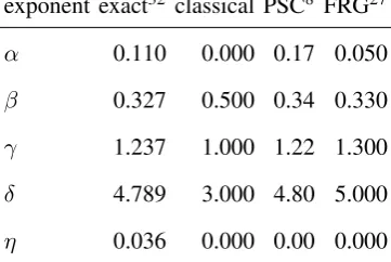
far from the critical density. The actual free energy of the system corresponds to the limitQ→0. Typically, the original free energy will have classical values of the critical exponents, which are
summarized in Table I. This renormalization process leads to a free energy with non-classical critical
exponents27, which are shown in the final column of Table I. Note that the critical exponentβ, which
is related to the shape of the coexistence curve, should not be confused with the inverse temperature
β = (kBT)−1. As a comparison, estimates of the “exact” values of the critical exponents32, as well as
the predictions from the phase-space cell renormalization method, are also shown.
APPLICATION TO A CUBIC EQUATION OF STATE
In order to concretely illustrate the utility of Eq. (18), we apply the approximate FRG method
a cubic equation which is widely used in industry to describe the thermodynamic properties of fluids
and fluid mixtures. The pressure is given by
p= ρkBT 1−ρb−
ρa(T)
1 +ρb (19)
wherea(T)is a temperature dependent parameter relating to the strength of the intermolecular attrac-tions, andbis a parameter relating to the size of the molecules. The corresponding expression for the
Helmholtz free energy density is
f(ρ, T)b= (ρb)(lnρb−1)−(ρb) ln(1−ρb)−(ρb)βa(T)
b ln(1 +bρ). (20)
The critical point of the SRK equation of state is33,34
kBTcb/a(Tc) = 0.202677
pcb2/a(Tc) = 0.0175999
ρcb= 0.259921
whereTcis the critical temperature,pcis the critical pressure, andρcis the critical density. The critical
compressibility factor for this equation of state isZc= 1/3. The vapor-liquid coexistence curve of the
SRK equation is shown in as the dashed line in Fig. 1(a). Because the SRK equation is analytical at
the critical point, it has a critical exponentβ = 0.5— the classical value. As a result, the coexistence curve has a shape which is much too sharp as compared to that typically found experimentally.
In order to apply the renormalization group transformation to the model free energy, the parameters
Λ andB must first be specified. The parameterΛrepresents the length scale for which fluctuations have already been incorporated in the classical free energy. For this, we expectΛb1/3 of the order or
smaller than one and use it as a dimensionless parameter that can be varied. The parameterB which
appears in the free energy functional shown in Eq. (14) relates to the gradient term of the density.
Consequently, we expect it to be proportional to the strength of the intermolecular interactions. In
addition, its range should be on the order on which the fluctuations have already been captured in the
system. Therefore, for the SRK equation of state, we selectB as
B =βa(T)Λ−2B¯ (21)
where B¯ is a dimensionless parameter, which can be adjusted to fit experimental data, and β = (kBT)−1.
The nonlinear partial differential equation in Eq. (18) is solved using the method of lines. The
partial derivatives of the free energy with respect to density are performed using the central difference
method. The resulting set of first-order ordinary differential equations are solved using the
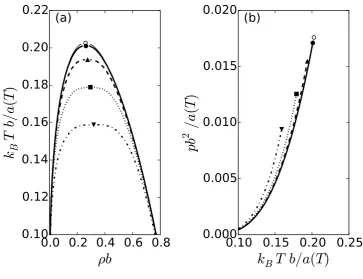
Figure 1 shows the vapor-liquid phase diagram as predicted by the SRK equation of state and
as modified by the renormalization group transformation given by Eq. (18). In this figure, the B¯
parameter is held fixed, while Λb1/3 is varied. Note that we assume that density fluctuations with a
wavelength smaller than2π/Λhave already been incorporated into the original free energy. Applying the renormalization group process will incorporate density fluctuations of larger wavelengths2π/Qby
integrating the flow equation, Eq. (18), overQtowards increasingly smaller values. If the parameter
Λis set to zero, then the original free energy is retained because all size fluctuations have already been
incorporated. The larger the value of Λ, the more fluctuations need to be added to the original free energy, which tends to have a stabilizing influence. From Fig. 1(a), we see that increasing the value
ofΛdecreases the critical temperature and increases the flatness of the vapor-liquid phase envelope.
This is a consequence of increasing the size of the critical region. Inside the critical region, the
system is dominated by fluctuations, and the value of the critical exponentβ (which is equal to0.330 within the approximate FRG method that is used in this work) dictates the shape of the vapor-liquid
coexistence curve. Outside this region, the shape of the coexistence curve is well described by
mean-field theory, which hasβ = 0.5, leading to a “sharper” shape. In addition, the coexistence pressure
tends to increase (see Fig. 1(b)).
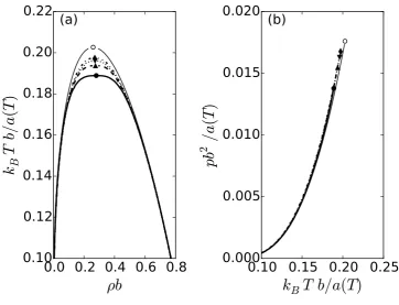
The affect of varying the parameter B, while holding¯ Λ fixed, on the phase diagram is shown in Fig. 2. Increasing the value of B¯ decreases the critical temperature, gradually flattening the top
of vapor-liquid phase envelope. Recall that the B parameter is the prefactor to the gradient term in
the free energy functional (see Eq. (14)). It gives a penalty for variations in the density distribution
in the system: large values of this parameter disfavor density fluctuations. Therefore, increasing
¯
B suppresses these stabilizing fluctuations and, consequently, increases the size of the vapor-liquid
coexistence region.
The parameter B¯ does not have as pronounced an affect on the vapor pressure curve, as on the coexistence phase envelope (see Fig. 2(b)). The vapor pressure curves calculated with different values
ofB¯appear to be quite similar, although they stop at lower values of the pressure and temperature for
larger values ofB¯.
THE INFLUENCE OF INTRAMOLECULAR CORRELATIONS
The renormalization group method described above accounts for large scale density fluctuations,
where different sections of the system are coupled mainly by intermolecular interactions. The
ex-tent and strength of these correlations are characterized by the parameter B. However, the method
does not account for other types of correlations that may occur in the system. In the case of chain
them. While at moderate to high monomer concentrations these correlations are typically screened
down to monomer length scales, at low densities, these correlations extend to the size of the molecules,
which for polymers or other macromolecules can be much larger than the monomer size.
These correlations tend to reduce the density fluctuations in the system36. In the renormalization
group methods developed to correct the critical behavior of classical free energies for simple liquids
(such as the phase-space cell method or the method described in the previous section of this work), the
correlations due to intramolecular bonding are neglected. As a consequence, attempting to empirically
adjust the parameters of the method to fit empirical or simulation data can lead to anomalies, such as
the vapor-liquid coexistence curve being much too flat (e.g., see Figs. 1 and 7 in Ref. 15 or Fig. 5 in
Ref. 16).
To better understand the influence of chain connectivity on the correlations in a solution, we
exam-ine an ideal gas of lexam-inear chains, each consisting ofN bonded monomers. In this case, the scattering
functionS(q)of the monomers in the system36
S(q)≈N[1 +q2R2g/3 +· · ·]−1 (22)
where Rg is the radius of gyration of the molecules, and ρ is the monomer number density. The
corresponding expression for the direct correlation function is
ρ−1−ˆc(q)≈ 1
N ρ[1 +q
2R2
g/3 +· · ·] (23)
The prefactor outside the square brackets on the right of Eq. (23) represents the inverse isothermal
compressibility of an ideal gas. This characterizes the strength of the monomer density fluctuations
in the system. The second term inside the square brackets denotes the influence of bonding on the
correlations in the system.
Generalizing this ideal gas expression for the direct correlation function to a system where the
monomers have size and interact, we find36
ρ−1−cˆQ(q) =fQ00(ρ) +Bq 2+1
3 R2g N ρq
2+· · ·
(24)
The first two terms in Eq. (24) are precisely the same as those for the simple liquid. The third term
represents the correlations in the system due to the connectivity of the monomers in the chain. At low
densities, the connectivity induces correlations in the monomer density profile on length scales larger
than the monomer size. As the density increases, these correlations are screened, with a characteristic
decay lengthλthat varies as36:
λ2 = 1 3
R2 g
Substituting this expression for the direct correlation function into Eq. (13), we can again
analyti-cally evaluate the integral overq. In this case, the flow equation for the free energy becomes:
Q∂fQ ∂Q =
KdBQ5
(fQ00 +BQ2)
3 (Ql)2
1− 1
QlarctanQl
(25)
whereξ2 = Rg2/(3N)is a length scale relating to a scaled size of the molecules in the system, and l2 =ρ−1ξ2/(f00
Q+BQ2).
In the limit that the molecules are small compared to the other correlation lengths in the system,
ξ → 0, and this equation reduces to Eq. (18). The critical corrections only become significant when the wavelength of the density fluctuations becomes larger than the size of the molecules (which may
be much larger than the monomer size).
APPLICATION TO CHAIN MOLECULES
In this section, the properties of linear chains composed of atoms interacting through the
Lennard-Jones potential (whereε is the energy scale, andσ is the size parameter) are examined. Each chain
in the system consists of N Lennard-Jones atoms bonded to each other with a bond length l. The
thermodynamics of the system is modeled using the first order thermodynamic perturbation theory
(also referred to as the soft-SAFT theory) developed by Johnson and coworkers37.
The Helmholtz free energy is considered to be composed of a contribution from a fluid of
discon-nected Lennard-Jones atomsfref and a contribution due to the bonding of the atoms within the chains.
The resulting expression for the residual Helmholtz free energy densityfres(the difference between
the Helmholtz free energy density of the system and that of an ideal gas at the same temperature and
density) is
fres=fref +fchain. (26)
wherefref is the residual Helmholtz free energy density of a Lennard-Jones monomer fluid, andfchain
is the chain bonding contribution to the Helmholtz free energy density of the chain system.
The free energy of the monomer Lennard-Jones fluid is computed from the equation of state
de-veloped by Johnson and coworkers38. The chain contribution is given by the work required to hold
two Lennard-Jones atoms together at a distance of the bond lengthl in the monomer fluid:
fchain = ρ
N(N −1) lny
ref(l)
whereyref is the indirect correlation function of the disconnected Lennard-Jones fluid. The
mathe-matical form for this term is taken from Ref. 37.
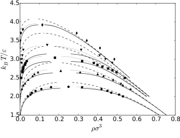
The predictions of the first order thermodynamic perturbation theory (TPT) for the vapor-liquid
in Fig. 3. The corresponding Monte Carlo simulation data39,40 are given by the symbols. TPT
con-sistently predicts a much larger coexistence region and a higher critical temperature than found by
simulation.
We apply the functional RG method to a first order thermodynamic perturbation theory
approxi-mation for the free energy. For the chains with N = 4, 8, 16, and32, the solid lines are the results of the RG transformation with the parametersΛσ = 1, BΛ2/(βεσ3) = 5, and ξ/σ = 0. While the RG predictions are reasonably good forN = 4, they get progressively worse asN increases for these
fixed values of the parameters, severely underestimating the height of the coexistence curve.
For the same chain lengths, the dotted lines for the RG transformation with the parametersΛσ = 1, BΛ2/(βεσ3) = 5, andξ/σ = 0.5. By adding the size correction, given by the parameterξ, the low density arm of the coexistence curve shifts slightly up and to the left, leaving the high density arm
relatively unmoved for the longer chain lengths. These curves are able to describe the coexistence
curve fairly well for all these chain lengths.
For the case N = 100shown in Fig. 3, the solid line corresponds to the RG transformation with Λσ = 0.5, BΛ2/(βεσ3) = 5, and ξ/σ = 0, and the dotted line corresponds to the parameters
Λσ = 0.5, BΛ2/(βεσ3) = 5, andξ/σ = 0.5. Based on these results, it appears that to get a good
description of the phase behavior of chain molecules, the parameterΛshould decrease slightly with chain length.
CONCLUSIONS
In this work, we have examined the application of a simple functional renormalization group
method to provide fluctuation corrections for classical free energy models. This method can be readily
applied to any model to better reproduce the non-analytical behavior of the thermodynamic properties
near the critical point.
In this work, we only illustrated the applicability of the functional renormalization group method
to general classical free energy models that are commonly used by engineers to describe fluid
ther-modynamic properties. The quantitiesΛ,B, andξappearing in the flow equation (see Eq. (25)) have
been left as adjustable parameters. This approach does, however, have a more rigorous molecular
basis, and, in principle, the parameters can be linked more closely to the molecular features of the
system.
More sophisticated approximations for the renormalizing free energy functional, beyond the
sim-ple gradient approximation28, can be used to obtain a more rigorous approach. However, this would
come at a cost of increased complexity and computational burden.
intramolecular correlations which result from bonds between atoms within a molecule. These
cor-relations tend to suppress the density fluctuations in the system and, as a consequence, shrink the
critical region. The neglect of this effect when applying the renormalization group method to systems
composed of large molecules has probably led to the calculation of vapor-liquid coexistence curves
that are much too flat compared to that observed experimentally. By including intramolecular
corre-lations, the FRG method is able to provide a good description of phase behavior of Lennard-Jones
chain fluids, as compared to computer simulation results.
One of the key practical limitations of current RG corrections has been the practical difficulties
in applying these methods to mixtures. While most of these methods can be straightforwardly
gen-eralized to account for multicomponent systems, such as the phase-space cell approximation and the
functional renormalization group approach described here, they rapidly become impractical as the
number of components in the system increases. This severely limits their usefulness in addressing
real engineering problems. It is hoped that in presenting this different approach to implementing the
renormalization group idea may stimulate new approximate methods to attacking multicomponent
systems.
REFERENCES
1Kiselev S. Cubic crossover equation of state. Fluid Phase Equil. 1998;147(12):7 – 23.
2Wyczalkowska AK, Anisimov MA, Sengers JV. Global crossover equation of state of a van der
Waals fluid. Fluid Phase Equil. 1999;158-160:523–535.
3Behnejad H, Cheshmpak H, Jamali A. The Extended Crossover Peng-Robinson Equation of State
for Describing the Thermodynamic Properties of Pure Fluids. J Stat Phys. 2015;158(2):372–385. 4Kiselev SB, Ely JF, Lue L, Elliott JR. Computer simulations and crossover equation of state of
square-well fluids. Fluid Phase Equil. 2002;200:121–145.
5Kiselev S, Ely J, Adidharma H, Radosz M. A crossover equation of state for associating fluids.
Fluid Phase Equil. 2001;183-184:53–64.
6Kiselev SB, Ely JF, Tan SP, Adidharma H, Radosz M. HRX-SAFT Equation of State for Fluid
Mixtures: Application to Binary Mixtures of Carbon Dioxide, Water, and Methanol.Ind Chem Res. 2006;45(11):3981–3990.
7Wilson KG. Renormalization Group and Critical Phenomena. I. Renormalization Group and the
Kadanoff Scaling Picture. Phys Rev B. 1971;4:3174–3183.
8Wilson KG. Renormalization Group and Critical Phenomena. II. Phase-Space Cell Analysis of
Critical Behavior. Phys Rev B. 1971;4:3184–3205.
of simple fluids. J Chem Phys. 1992;96(6):4559–4568.
10White JA, Zhang S. Renormalization group theory for fluids.J Chem Phys. 1993;99(3):2012–2019. 11White JA, Zhang S. Renormalization theory of nonuniversal thermal properties of fluids. J Chem
Phys. 1995;103(5):1922–1928.
12Lue L, Prausnitz JM. Renormalization-group corrections to an approximate free-energy model for
simple fluids near to and far from the critical region. J Chem Phys. 1998;108(13):5529–5536. 13Lue L, Prausnitz JM. Thermodynamics of fluid mixtures near to and far from the critical region.
AIChE J. 1998;44(6):1455–1466.
14Fornasiero F, Lue L, Bertucco A. Improving cubic EOSs near the critical point by a phase-space
cell approximation. AIChE J. 1999;45(4):906–915.
15Llovell F, P`amies JC, Vega LF. Thermodynamic properties of Lennard-Jones chain molecules:
Renormalization-group corrections to a modified statistical associating fluid theory. J Chem Phys. 2004;121(21):10715–10724.
16Forte E, Llovell F, Vega LF, Trusler JPM, Galindo A. Application of a renormalization-group
treatment to the statistical associating fluid theory for potentials of variable range (SAFT-VR). J Chem Phys. 2011;134(15):154102.
17Forte E, Llovell F, Trusler JM, Galindo A. Application of the statistical associating fluid theory
for potentials of variable range (SAFT-VR) coupled with renormalisation-group (RG) theory to
model the phase equilibria and second-derivative properties of pure fluids.Fluid Phase Equil. 2013; 337:274–287.
18Lue L, Friend DG, Elliott JR. Critical compressibility factors for chain molecules.Mol Phys. 2000; 98(18):1473–1477.
19Lue L. Equation of state for polymer chains in good solvents. J Chem Phys. 2000;112(7):3442– 3449.
20Patrickios CS, Lue L. Equation of state for star polymers in good solvents. J Chem Phys. 2000; 113(13):5485–5492.
21Parola A, Pini D, Reatto L. Liquid-Vapor Transition from a Microscopic Theory: Beyond the
Maxwell Construction. Phys Rev Lett. 2008;100:165704.
22Parola A, Pini D, Reatto L. The smooth cut-off hierarchical reference theory of fluids. Mol Phys. 2009;107(4-6):503–522.
23Parola A, Reatto L. Recent developments of the hierarchical reference theory of fluids and its
relation to the renormalization group. Mol Phys. 2012;110(23):2859–2882.
24Parola A, Pini D. Liquid-vapour transition in screened Coulomb binary mixtures. Mol Phys. 2011; 109(23-24):2989–2999.
26Caillol JM. Link between the hierarchical reference theory of liquids and a new version of the
non-perturbative renormalization group in statistical field theory. Mol Phys. 2011;109(23-24):2813– 2822.
27Ionescu CD, Parola A, Pini D, Reatto L. Smooth cutoff formulation of hierarchical reference theory
for a scalarφ4 field theory. Phys Rev E. 2007;76:031113.
28Hansen JP, McDonald IR. Theory of Simple Liquids. London: Academic Press, 2nd ed. 1986. 29Litim DF. Mind the gap. Int J Mod Phys A. 2001;16(11):2081–2087.
30Litim DF. Optimized renormalization group flows. Phys Rev D. 2001;64:105007.
31Baus M, Lovett R. A direct derivation of the profile equations of Buff-Lovett-Mou-Wertheim from
the Born-Green-Yvon equations for a non-uniform equilibrium fluid. Physica A. 1992;181(34):329 – 345.
32Pelissetto A, Vicari E. Critical phenomena and renormalization-group theory. Phys Rep. 2002; 368(6):549 – 727.
33Redlich O, Kwong JNS. On the Thermodynamics of Solutions. V. An Equation of State. Fugacities
of Gaseous Solutions. Chem Rev. 1949;44(1):233–244.
34Soave G. Equilibrium constants from a modified Redlich-Kwong equation of state. Chem Eng Sci. 1972;27(6):1197 – 1203.
35Hindmarsh AC, Brown PN, Grant KE, Lee SL, Serban R, Shumaker DE, Woodward CS.
SUN-DIALS: Suite of Nonlinear and Differential/Algebraic Equation Solvers. ACM Trans Math Softw. 2005;31(3):363–396.
36Grosberg AY, Khokhlov AR. Statistical Physics of Macromolecules. Woodbury: AIP Press. 1994. 37Johnson JK, Mueller EA, Gubbins KE. Equation of State for Lennard-Jones Chains. J Phys Chem.
1994;98(25):6413–6419.
38Johnson JK, Zollweg JA, Gubbins KE. The Lennard-Jones equation of state revisited. Mol Phys. 1993;78(3):591–618.
39Escobedo FA, de Pablo JJ. Simulation and prediction of vapour-liquid equilibria for chain
molecules. Mol Phys. 1996;87(2):347–366.
40Sheng YJ, Panagiotopoulos AZ, Kumar SK, Szleifer I. Monte Carlo calculation of phase equilibria
LIST OF FIGURE CAPTIONS
Figure 1 The vapor-liquid coexistence curve (a) and the vapor pressure (b) as determined by the
Soave-Redlich-Kwong (SRK) equation of state and the renormalization group with B¯ = 1 and (i) Λb1/3 = 0.5 (solid line, filled circle), (ii) Λb1/3 = 1 (dashed line, filled triangle up), (iii)
Λb1/3 = 1.5(dotted line, filled square), and (iv) Λb1/3 = 2(dashed-dotted line, filled triangle
down). The thin solid line is for the SRK equation of state. The symbols denote the critical
point. The open circle denotes the critical point of the SRK equation of state.
Figure 2 The vapor-liquid coexistence curve (a) and the vapor pressure (b) as determined by the
Soave-Redlich-Kwong (SRK) equation of state and the renormalization group withΛb1/3 = 1and (i) ¯
B = 0.5 (solid line, filled circle), (ii)B¯ = 1 (dashed line, filled triangle up), (iii)B¯ = 1.5
(dotted line, filled square), and (iv)B¯ = 2(dashed-dotted line, filled triangle down). The thin solid line is for the SRK equation of state. The symbols denote the critical point. The open
circle denotes the critical point of the SRK equation of state.
Figure 3 Vapor-liquid coexistence curve for linear chains composed of (i) N = 4 (circles), (ii) N = 8 (triangles up), (iii) N = 16 (squares), (iv) N = 32 (triangles down), and (v) N = 100
(diamonds), Lennard-Jones atoms. The symbols are Monte Carlo simulation data from Refs. 39
and 40, the dashed lines are the predictions of the TPT, and the solid and dotted lines are from
0.0 0.2 0.4 0.6 0.8
ρb
0.10 0.12 0.14 0.16 0.18 0.20 0.22
k
BT
b/
a(
T)
(a)
0.10 0.15 0.20 0.25
k
BT b/a(T)
0.000 0.005 0.010 0.015 0.020
pb
2
/a
(T
)
[image:17.595.115.479.65.344.2](b)
0.0 0.2 0.4 0.6 0.8
ρb
0.10 0.12 0.14 0.16 0.18 0.20 0.22
k
BT
b/
a(
T)
(a)
0.10 0.15 0.20 0.25
k
BT b/a(T)
0.000 0.005 0.010 0.015 0.020
pb
2
/a
(T
)
[image:18.595.116.479.65.342.2](b)
0.0 0.1 0.2 0.3 0.4 0.5 0.6 0.7 0.8
ρσ
31.5 2.0 2.5 3.0 3.5 4.0 4.5
k
BT/
[image:19.595.117.478.69.344.2]ε
LIST OF TABLES
TABLE I. Estimates of the critical exponents from the phase-space cell (PSC) approximation and the functional
renormalization group (FRG) method.
exponent exact32 classical PSC8 FRG27
α 0.110 0.000 0.17 0.050
β 0.327 0.500 0.34 0.330
γ 1.237 1.000 1.22 1.300
δ 4.789 3.000 4.80 5.000