Multi-objective optimization of hyperelastic material constants : a feasibility study

1 INTRODUCTION

The ability to accurately simulate a component’s be-havior allows the engineer to gain a greater under-standing of its expected service life. To do this suc-cessfully, the conditions the component is exposed to (structural and/or thermal) must be known, along with the corresponding material properties. In the case of rubber components, the description of a giv-en material requires indepgiv-endgiv-ent characterization due to the variation in properties resulting from chemical composition, processing and manufactur-ing methods. In addition, the stress-strain response of rubber is highly nonlinear and dependent on the applied mode of deformation, requiring measure-ment of its multi-axial response.

Hyperelastic material models are widely used in simulation or mathematical descriptions of the static response of rubber. These may have a micro-mechanical or phenomenological bases. Although the former is physical in its formulation, both ap-proaches typically require the same degree of testing to calibrate the response. Compressibility effects may be taken into account by partitioning the de-formation gradient into isochoric and deviatoric components, which requires an additional confined compression experiment. Models of more complex isothermal behaviors experienced by rubbers, such as the Mullins effect with permanent set and induced anisotropy (Diani, et al., 2009), hysteresis and visco-elasticity (Bergstrom & Boyce, 1999), are usually based on hyperelastic models. The remainder of this paper’s content will study the isothermal and

quasi-static material response of rubber and a novel meth-od to obtain hyperelastic constants from experi-mental data.

The most common method of characterizing the static and incompressible response of rubber is through performing three homogeneous tests: uniax-ial tension (UT), planar tension (PT) (equivalent to pure shear) and equibiaxial tension (ET). These tests were popularized by Treloar on 8% Sulphur rubber (Treloar, 1944) who collected the equibiaxial ten-sion, or 2-dimensional extenten-sion, data with the use of an inflated rubber sheet. Uniaxial and planar ten-sion data can both be collected using cut rubber sheets of simple geometry and a commonplace uni-axial testing machine. However, equibiuni-axial testing requires some form of bespoke testing equipment usually in the form of simultaneous loading of per-pendicular axes within a 2D plane or perper-pendicularly applied inflation and punch tests.

Due to the difficulty of applying equibiaxial load-ing and gainload-ing accurate results, several different methods have been developed to obtain this data. One method is to adapt a uniaxial testing machine with a device that translates a controlled ratio of the applied vertical force horizontally (Brieu, et al., 2006). The difficulty in this method is in achieving a homogeneous equibiaxial response, as the chosen geometry of the sample will affect the degree of biaxiality (Seibert, et al., 2014). Alternatively, a load can be applied radially to a circular sample using a complex pulley system. Other methods use inhomogeneous deformations and advanced imaging

Multi-objective optimization of hyperelastic material constants: a

feasibility study

S. Connolly, D. Mackenzie & T. Comlekci

Department of Mechanical & Aerospace Engineering, University of Strathclyde, Glasgow, UK

techniques to extract the required equibiaxial material response (Sasso, et al., 2008).

In this study, a multi-objective optimization pro-cedure was developed to determine whether hypere-lastic material constants can be obtained by an alter-native method. Standard homogeneous tests are represented by simple finite element representations for use in the optimization process to obtain the op-timal hyperelastic constants. If successful, this method will be extended to efficiently gain opti-mized material constants using simple inhomogene-ous test data and equivalent finite element simula-tions.

2 OPTIMIZATION METHODOLOGY 2.1 Material data and modelling

Treloar’s data for UT, PT & ET tests from (Steinmann, et al., 2012) were adopted for use in this optimization procedure. This data set is commonly used as a benchmark in the development and valida-tion of hyperelastic material models.

Comparison studies investigating several material models in terms of the best fit to the entire data set (Marckmann & Verron, 2006) and the best fit to all data sets using data from a single test (Steinmann, et al., 2012, Hossain & Steinmann, 2013) indicate that the micro-mechanical extended-tube model (Kaliske & Heinrich, 1999) performed best overall. The best phenomenological model was the third-order Ogden model (Ogden, 1972) with six material constants, alhough this model is incapable of predicting other data sets when only one test’s data was used.

Ideally, the extended-tube and third-order Ogden material models would therefore be used in this study, however, the extended-tube model was not available at the time of study and required a UHYPER or UMAT subroutine for its implementation. Therefore, the third-order Ogden model was used along side a third-order Yeoh model (Yeoh, 1993), which is a hybrid micro-mechanical model with a phenomenological adjustment. Since the number of coefficients is proportional to the time required for the optimization process, with only three material constants, the third-order Yeoh model provided an initial insight into the feasibility of the chosen optimization methods and a suitable comparison.

2.2 Finite element modelling

For each mode of deformation, an Abaqus input script was generated with only a single millimeter cubed element. Within this script, the hyperelastic constants were parameterized such that they could be easily identified and controlled by the optimizer. Displacement boundary conditions were applied for each variation to the appropriate nodes, shown for

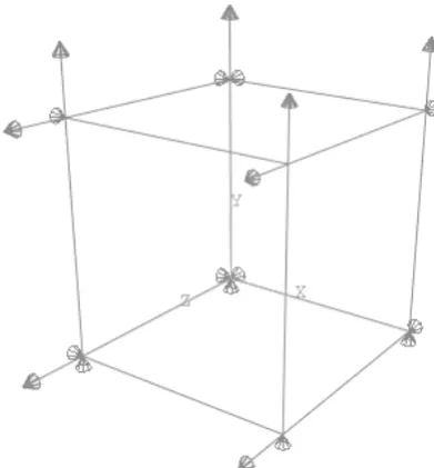
the case of equibiaxial tension in Figure 1. With dis-placements applied in millimeters, the nodal force reaction was extracted along with the nodal dis-placement to give stress and strain results in MPa and mm/mm respectively. Though the extracted force from a single node gives only a quarter of the actual stress value, the matched data was conse-quently quartered for comparison.

Figure 1. Equibiaxial Tension boundary conditions for the sin-gle element simulated model

2.3 Optimization method

The optimization procedure is performed automati-cally using a combination of two Simulia products: Abaqus and Isight. Abaqus is used for the simulation of the input set of hyperelastic constants using the simple finite element models, discussed in section 2.2. Isight is responsible for assessing and directing the input of the hyperelastic constants based on the results of the comparison of the error between the fi-nite element results and the experimental data sets. As there are multiple data sets, one for each mode of deformation, the optimization process is therefore multi-objective and a weight function is used to en-sure that the error of each data set’s magnitude is normalized. For all optimizations, the absolute dif-ference (error) function is used.

nomi-nal strain range: -0.9 ≤ ε ≤ 9.0, using the Drucker stability criterion. (Abaqus, 2016)

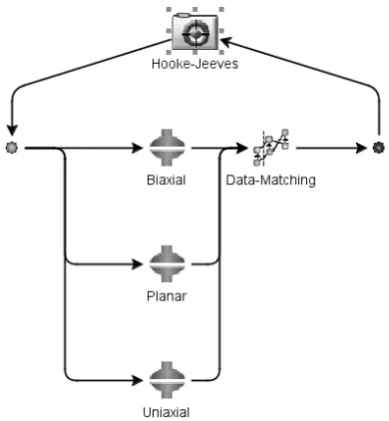
In the selection of the optimization method, two distinct variations were used: the first used initial guesses based on the values obtained by the Abaqus evaluation and employed an optimization algorithm; the second method used trivial starting points and wide-ranging bounds with a hybrid optimization-exploratory algorithm. In the former, the Hooke-Jeeves algorithm (Hooke & Hooke-Jeeves, 1961) was used due to its ability to find local minima. As for the lat-ter, the parallel Pointer-2 algorithm (Van der Velden & Koch, 2010) was selected. Pointer-2 is an algorithm that controls four optimisation methods in serial or in parallel, ensuring that the design space is explored and most, if not all, minima are found within it. The Isight optimisation process for the Hooke-Jeeves method is shown in Figure 2.

Figure 2. Hooke-Jeeves multi-objective optimization within Isight

3 OPTIMIZATION RESULTS

For both material models, an optimization using each method was attempted. In the case of the Hooke-Jeeves optimization, which is somewhat de-pendent on the chosen starting point, the initial ma-terial constants were chosen to within one decimal point of the evaluated constant from Abaqus. As for the upper and lower bounds, the nearest whole inte-ger was used rounding upwards and downwards re-spectively. In the Pointer-2 optimization, the starting points were chosen arbitrarily and the constants were bound by a wide range.

The solutions found to be optimal for the fit of all data sets were compared in terms of the absolute dif-ference (error) function used for the optimization. Stress-strain graphs were plotted to visually assess their fit to the material data. In the presentation of the results, the following abbreviations are used:

Er-ror: absolute difference (error), Abq: Abaqus evalu-ated results, H-J: Hooke-Jeeves and P-2: Pointer-2. Other symbols used are the common notations for the hyperelastic material constants or have been pre-viously defined.

3.1 3rd_{-order Yeoh}

Given that the third-order Yeoh model was not ranked as a highly accurate model in the referenced comparison studies, it was not expected to achieve as close a fit as the Ogden model. This was observed to be the case in the initial Abaqus evaluation of the material models. The Hooke-Jeeves model was ca-pable of gaining a better fit to the data, in terms of average error and the Pointer-2 optimization gained solutions with a significantly smaller error value. Solutions for the Pointer-2 and Hooke-Jeeves opti-mizations are shown in Table 1, along with the Abaqus evaluated results. The Drucker stability check revealed that all sets were stable for the as-sessed nominal strain range.

Table 1. Hyperelastic constants and absolute difference (error) for third-order Yeoh optimizations

___________________________________________________ Yeoh: Abq H-J P-2 ___________________________________________________ c10 0.1852 0.1740 0.2032 c20 (E-3) -1.449 -3.242E-3 -2.786 c30 (E-5) 3.973 2.460 6.847 ___________________________________________________ Average Error 1.407 1.298 1.097 ___________________________________________________ ET Error 2.367 0.8590 1.767 PT Error 0.4686 1.582 0.6573 UT Error 1.386 1.453 0.8663 ___________________________________________________

Figure 3. Third-order Yeoh quartered stress-strain plot

3.2 Third-order Ogden

The third-Ogden model was expected to capably achieve a solution for the simpler Hooke-Jeeves method. However, the Pointer-2 method was less likely to achieve the desired result due to the vast number of numerical combinations with six coeffi-cients. After running the Pointer-2 optimization for a 24 hour period, the program was stopped and the best result was taken. As can be seen in Table 2, the result is significantly worse than the Abaqus and Hooke-Jeeves results, in terms of absolute difference (error), for all data sets. This set was also found to be unstable in uniaxial tension greater than ε = 3.08 and, the equivalent deformation mode, in biaxial compression less than ε = -0.505. The other sets were completely stable over the assessed range.

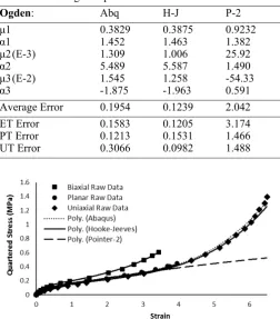
Table 2. Hyperelastic constants and absolute difference (error) for third-order Ogden optimizations

___________________________________________________ Ogden: Abq H-J P-2

___________________________________________________

μ1 0.3829 0.3875 0.9232

α1 1.452 1.463 1.382

μ2 (E-3) 1.309 1.006 25.92

α2 5.489 5.587 1.490

μ3 (E-2) 1.545 1.258 -54.33

α3 -1.875 -1.963 0.591 ___________________________________________________ Average Error 0.1954 0.1239 2.042 ___________________________________________________ ET Error 0.1583 0.1205 3.174 PT Error 0.1213 0.1531 1.466 UT Error 0.3066 0.0982 1.488 ___________________________________________________

Figure 4. Third-order Ogden quartered stress-strain plot

The stress-strain results of the third-Ogden opti-mization are shown in Figure 4. As previously, the optimization results are plotted using sixth-order polynomials. Both the Abaqus and Hooke-Jeeves re-sults are a good fit of the entire data set. However, as suggested by the numerical error, the Pointer-2 set did not manage to gain a suitable set of coefficients within the prescribed time. If run for long enough, a comparable or better result would be obtained. However, the required time for a solution would not be a feasible alternative means for material charac-terization.

3.3 Observations

The third-order Ogden model produced a signifi-cantly better fit of the data than the third-order Yeoh model. However, with six coefficients, the Ogden model did not gain a suitable solution with the ex-ploratory method. When viewing the sets of coeffi-cients produced within the Pointer-2 optimization, the constants of the Ogden model were found to fluctuate significantly for solutions with similar magnitudes of error. This demonstrates that a unique set of constants may not exist for the third-order Og-den model for this data set due to it being phenome-nological in nature, which is in agreement with Og-den et al (OgOg-den, et al., 2004). This is shown in Figure 5, where the magnitude of the third-order Ogden coefficients are plotted for five solutions with similar error. This suggests that, where an approxi-mate initial guess is not known, mechanically based models with fewer coefficients are preferable.

Figure 5. Third-order Ogden coefficients plotted for five opti-mization results with similar error

4 NOVEL MATERIAL CHARACTERISATION METHOD

This method, if successful, could provide an alter-native to bespoke equibiaxial testing equipment when gathering the multi-axial response for rubber-like materials. The data to capably characterize the incompressible, static response is hypothesized to use three tests: uniaxial tension, planar tension and bonded uniaxial compression tests. The benefit of these tests is that they can all be performed using the same uniaxial testing machine, provided it is capable of producing the required loads in both tension and compression. Additionally, the required specimens are of simple geometry and easy to manufacture.

The accuracy of the method is largely dependent on both the experimental results and finite element results. The finite element results will be of approx-imately comparable accuracy to the material model’s limitations, provided that finite element phenomena are appropriately considered, notably mesh conver-gence and volumetric-locking in this instance. How-ever, the experimental error may be increased due to the inclusion of inhomogeneous tests. These may re-quire significantly more cycling before a consistent response is attained, due to the propagation of stress-softening through the specimen, owing to the Mullin’s effect. Also, the strain-rate will be some-what variant throughout the material and will require consideration for the different tests to be consistent in this regard.

In order to validate this method, it will be im-portant to use material models to generate simulated equibiaxial data for comparison to equibiaxial data gathered in a more conventional form. Also, it will be necessary to use compression specimens of dif-ferent diameter to provide further validation and demonstrate repeatability.

5 CONCLUSIONS

Using Treloar’s data and two multi-objective opti-mization techniques, the feasibility of integrating these techniques in an alternative method for materi-al characterization has been investigated. The results of this study have found that a suitable initial value and approximate bounds for the hyperelastic coeffi-cients is of significant importance. Also, higher-order phenomenological models are expected to be less appropriate unless an optimization process that exploits local minima is used.

In gaining optimized constants, the Hooke-Jeeves method was more efficient than the Pointer-2 meth-od, as would be expected. However, the time taken to gain a solution using either multi-objective opti-mization method is substantially longer than the Abaqus evaluation tool. A significant portion of the time required is spent in ‘housekeeping’ tasks within Abaqus, some examples are: accessing the license server, writing the results files and reading output database files. For this type of optimization, the

simple homogeneous deformations of the unit-cube models could be more efficiently simulated in a purely mathematical form.

6 ACKNOWLEDGEMENTS

This project was supported in full by an EPSRC Studentship grant related to (EP/N509760/1).

7 REFERENCES

Abaqus 2016. v2016 User's Manual, Dassault Systèmes, Provi-dence, RI, USA

Bergstrom, J. S. & Boyce, M. C., 1999. Mechanical behavior of particle filled elastomers. Rubber chemistry and technol-ogy, 72(4), pp. 633-656.

Brieu, M., Diani, J. & Bhatnagar, N., 2006. A New Biaxial Tension Test Fixture for Uniaxial Testing Machine - A Val-idation for Hyperelastic Behavior of Rubber-like materials. Journal of Testing and Evaluation, 35(4), pp. 1-9.

Diani, J., Fayolle, B. & Gilormini, P., 2009. A review on the Mullins effect. European Polymer Journal, 45(3), pp. 601-612.

Hooke, R. & Jeeves, T., 1961. Direct Search Solution of Nu-merical and Statistical Problems. Journal of the ACM (JACM), 8(2), pp. 212-229.

Hossain, M. & Steinmann, P., 2013. More hyperelastic models for rubber-like materials: consistent tangent operators and comparative study. Journal of the Mechanical Behavior of Materials, 22(1-2), pp. 27-50.

Kaliske, M. & Heinrich, G., 1999. An extended tube-model for rubber elasticity: statistical-mechanical theory and finite el-ement implel-ementation. Rubber Chemistry and Technology, 72(4), pp. 602-632.

Marckmann, G. & Verron, E., 2006. Comparison of hyperelas-tic models for rubber-like materials. Rubber Chemistry and Technology, 79(5), pp. 835-858.

Ogden, R. W., 1972. Large Deformation Isotropic Elasticity - On the Correlation of Theory and Experiment for Incom-pressible Rubberlike Solids. Proceedings of the Royal Soci-ety of London A: Mathematical, Physical and Engineering Sciences, 326(1567), pp. 565-584.

Ogden, R. W., Saccomandi, G. & Sgura, I., 2004. Fitting hy-perelastic models to experimental data. Computational Me-chanics, 32(6), pp. 484-502.

Sasso, M., Palmieri, G., Chiappini, G. & Amodio, D., 2008. Characterization of hyperelastic rubber-like materials by biaxial and uniaxial stretching tests based on optical meth-ods. Polymer Testing, 27(8), pp. 995-1004.

Seibert, H., Scheffer, T. & Diebels, S., 2014. Biaxial testing of elastomers-Experimental setup, measurement and experi-mental optimization of specimen’s shape. Technische Mechanik, 34(2), pp. 72-89.

Steinmann, P., Hossain, M. & Possart, G., 2012. Hyperelastic models for rubber-like materials: consistent tangent opera-tors and suitability for Treloar’s data. Archive of Applied Mechanics, 82(9), pp. 1183-1217.

Treloar, L. R. G., 1944. Stress-strain data for vulcanised rubber under various types of deformation. Transactions of the Faraday Society, Volume 40, pp. 59-70.

Van der Velden, A. & Koch, P., 2010. Isight design optimiza-tion methodologies. ASM Handbook, Volume 22.