Implicit network descriptions of RLC networks and the problem of re-engineering

City, University of London Institutional Repository

Citation: Livada, M. (2017). Implicit network descriptions of RLC networks and the

This is the accepted version of the paper.

This version of the publication may differ from the final published

version.

Permanent repository link: http://openaccess.city.ac.uk/17916/

Link to published version:

Copyright and reuse: City Research Online aims to make research

outputs of City, University of London available to a wider audience.

Copyright and Moral Rights remain with the author(s) and/or copyright

holders. URLs from City Research Online may be freely distributed and

linked to.

City Research Online: http://openaccess.city.ac.uk/ [email protected]

Networks and the Problem of

Re-engineering

by

Maria Livada

A thesis submitted for the degree of Doctor of Philosophy (Ph.D.) in Control Theory

in the

Systems and Control Research Centre

School of Mathematics, Computer Science and Engineering

This thesis introduces the general problem of Systems Re-engineering and focuses to the special case of passive electrical networks. Re-engineering differs from classical control problems and involves the adjustment of systems to new requirements by intervening in an early stage of system design, affecting various aspects of the underlined system struc-ture that affect the final control design problem. Addressing problems of re-engineering requires the development of a system representation able to embody these structural changes. In the case of Re-engineering in passive electrical networks, certain types of re-engineering transformations involve alterations of values or nature of existing elements, modification of network’s topology and possible evolution of the network. We resort to the Implicit Network DescriptionW(s) as a unifying representation, which stems from the Impedance/Admittance integral-differential models, since it enables the representa-tion of such parametric and structural changes of the system as perturbarepresenta-tions on it. By using tools and results from classical network theory and algebraic systems theory, the thesis deals with the development and study of fundamental system aspects of this new description in terms of McMillan degree, regularity and other system properties of the implicit network description. The thesis also examines the effect of transformations that preserve network cardinality on the Implicit Network Description and particularly in the natural frequencies of the network. This leads to the formulation of Determinantal Frequency Assignment Problems for natural frequency improvements. Using the exte-rior algebra, algebraic geometry framework we prove sufficient conditions for complex frequency assignability for a special case of network transformations and we examine whether real solutions to the problem exist. Additionally, transformations linked to the variation of network cardinality, are represented as augmentation or reduction in terms of dimension of the Implicit Network Description and by identifying those that remain intact we are in position to define fixed dynamics, enabling the formulation of partial

Maria Livada City, University of London, July 18, 2017

Undertaking this PhD has been a truly life-changing experience for me and it would not have been possible to do without the support and guidance that I received from many people.

First and foremost, I would like to express my deepest gratitude to my supervisor Profes-sor N. Karcanias for giving me inspiration, motivation and guidance during my research studies. Without his supervision, immense knowledge and support the development of my Thesis would not have been possible and without his directions and suggestions on several aspects I would not have managed to overcome the difficulties faced during my research studies. In a more personal level, I would also like to acknowledge the moral support he provided me and the fact that he stood always by me throughout my years in London.

I also wish to pay special tribute to Dr. J. Leventides for sharing his knowledge with me, for his support and for his constructive suggestions during my research. The important work he has conducted along with his in-depth knowledge in the fields of Mathemat-ics and Control made the discussions we had invaluable and offered me the chance to consider from a different perspective the subject matter of this Thesis.

I also would like to thank all the members of the Research Control Centre in City, University of London for their excellent collaboration and feedback during this work. A special thanks to Dr. E. Milonidis and Professor G. Halikias for their collaboration along with moral support and understanding during the best and the worst of times. Moreover, I would like to acknowledge the external examiner, Professor G. Papavasilopoulos, for his comments and suggestions during Viva examination towards the improvement of my Thesis.

Finally, I would like to thank my family for standing by me everywhere, anywhere and for everything, regardless the distance and the circumstances and for believing in me. I am and will be grateful for life for everything you are doing for me. Last but not least, a great thanks goes to my friends, especially those who have or had a similar experience with mine, for being there for me when I needed them most, for all the good and bad times we had and for all their understanding and support throughout these years.

I, Maria Livada, hereby declare that this thesis titled, ‘Implicit Network Descriptions of RLC Networks and the Problem of Re-engineering’ and the work presented in it are my own. I also confirm that:

The work presented in this Thesis is my own unless stated and referenced in the

text accordingly.

Where I have consulted the published work of others, this is always clearly

at-tributed.

I have acknowledged all main sources of help.

I grant powers of discretion to the Librarian of City University London to allow

single copies of this Thesis for study purposes, subject to normal conditions of acknowledgement.

Signed:

Date:

List of Figures ix

List of Tables xi

Abbreviations xiii

Notation xv

1 Introduction 1

2 Systems and Mathematics Background 7

2.1 Introduction. . . 7

2.2 Background of Graph Theory and Properties . . . 8

2.3 Polynomial Matrices and Matrix Pencils . . . 14

2.4 Determinantal Assignment Problem . . . 20

2.5 Tools from Exterior Algebra . . . 23

2.6 Laplace Expansion Technique . . . 26

2.7 Complex, Real Varieties and Morphisms . . . 27

2.8 Intersection Theory of Complex Algebraic Varieties . . . 30

2.9 Conclusions . . . 37

3 Systems Re-engineering and Networks: Problem Statement, Litera-ture Review and Research Agenda 39 3.1 Introduction. . . 39

3.2 The Re-engineering Problem . . . 40

3.3 Review of Network Research. . . 45

3.4 Research Agenda: Systems Theory and Redesign of Internal Implicit Models 56 3.5 Conclusions . . . 57

4 Implicit Network Descriptions and Their Properties 59 4.1 Introduction. . . 59

4.2 Impedance Modeling, Loop Topology and Selection of Independent Loops 60 4.3 Admittance Modeling and Vertex Topology . . . 68

4.4 The Internal Network Operator W(s) and the Implicit Network Description 78 4.5 Relationship Between Impedance and Admittance Operators . . . 79

4.6 The Network Pencil and its Relationship to the Internal Network Descrip-tion . . . 82

4.7 Network Regularity and Invertibility of W(s) . . . 84

4.8 Natural Frequencies and the Network Pencil . . . 96

4.9 Conclusions . . . 102

5 Properties of Implicit Network Descriptions and The McMillan

De-gree 103

5.1 Introduction. . . 103

5.2 Implicit McMillan Degree and Its Calculation . . . 104

5.3 Necessary and Sufficient Conditions For Determining The Implicit McMil-lan Degree . . . 108

5.4 Graph Systematic Approach of Necessary and

Sufficient Conditions . . . 115

5.5 The Network Pencil P(s) and Links to the McMillan Degree of the Network121

5.6 Examples . . . 123

5.7 Conclusions . . . 133

6 System Transformations Preserving or Altering Network Cardinality

and Possibly the McMillan Degree 135

6.1 Introduction. . . 135

6.2 RLC Network Transformations Preserving McMillan Degree and Network Cardinality . . . 136

6.3 RLC Network Transformations Preserving Cardinality but Altering McMil-lan Degree . . . 142

6.4 RLC Network Transformations Altering Cardinality and the McMillan Degree . . . 145

6.5 Fixed Dynamics of RLC Networks under Network Transformations . . . . 158

6.6 Conclusions . . . 166

7 RLC Networks Redesign As Frequency Assignment Problems:

Cardi-nality Preserving Transformations 167

7.1 Introduction. . . 167

7.2 Frequency Assignment by Cardinality Preserving Transformations . . . . 168

7.3 Frequency Assignment in RLC Networks via Diagonal Perturbations . . . 170

7.4 A Cohomology Approach to Frequency Assignment . . . 179

7.5 Improving Natural Frequencies By Network Redesign: Frequency Assign-ment, Passivity and The Family Of Strongly Stable Polynomials . . . 188

7.6 Conclusions . . . 195

8 Conclusions and Future Research 197

8.1 Conclusions . . . 197

8.2 Future Research Work . . . 200

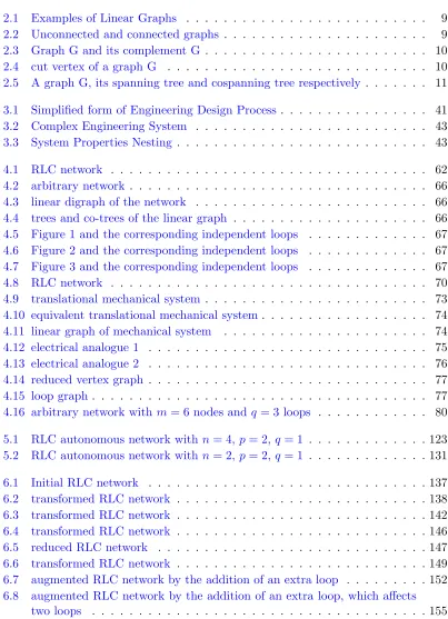
2.1 Examples of Linear Graphs . . . 9

2.2 Unconnected and connected graphs . . . 9

2.3 Graph G and its complement G . . . 10

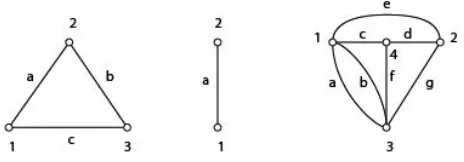
2.4 cut vertex of a graph G . . . 10

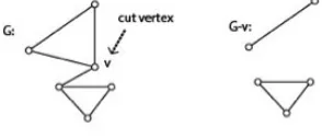
2.5 A graph G, its spanning tree and cospanning tree respectively . . . 11

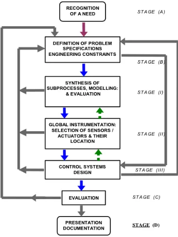
3.1 Simplified form of Engineering Design Process . . . 41

3.2 Complex Engineering System . . . 43

3.3 System Properties Nesting . . . 43

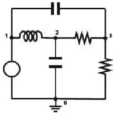
4.1 RLC network . . . 62

4.2 arbitrary network . . . 66

4.3 linear digraph of the network . . . 66

4.4 trees and co-trees of the linear graph . . . 66

4.5 Figure 1 and the corresponding independent loops . . . 67

4.6 Figure 2 and the corresponding independent loops . . . 67

4.7 Figure 3 and the corresponding independent loops . . . 67

4.8 RLC network . . . 70

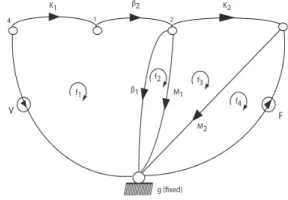
4.9 translational mechanical system . . . 73

4.10 equivalent translational mechanical system. . . 74

4.11 linear graph of mechanical system . . . 74

4.12 electrical analogue 1 . . . 75

4.13 electrical analogue 2 . . . 76

4.14 reduced vertex graph . . . 77

4.15 loop graph. . . 77

4.16 arbitrary network withm= 6 nodes and q = 3 loops . . . 80

5.1 RLC autonomous network withn= 4,p= 2,q = 1 . . . 123

5.2 RLC autonomous network withn= 2,p= 2,q = 1 . . . 131

6.1 Initial RLC network . . . 137

6.2 transformed RLC network . . . 138

6.3 transformed RLC network . . . 142

6.4 transformed RLC network . . . 146

6.5 reduced RLC network . . . 147

6.6 transformed RLC network . . . 149

6.7 augmented RLC network by the addition of an extra loop . . . 152

6.8 augmented RLC network by the addition of an extra loop, which affects two loops . . . 155

6.9 Network (1) . . . 158

6.10 Network (1a) . . . 159

6.11 Network (1b) . . . 160

6.12 Augmented Network (2a) . . . 161

6.13 Augmented Network (2b) . . . 161

6.14 Augmented Network (2c) . . . 162

6.15 Augmented Network (2d) . . . 162

1 Classification of pure elements. . . 204

cmi columnminimalindices

DAP Determinantal AssignmentProblem

FAP FrequencyAssignment Problem

IAI Impedance-AdmittanceImplicit

MFD MatrixFraction Description

QPR Quadratic Pl¨uckerRelations

PPM PolePlacement Map

RLC Resistance, Inductance, Capacitance

rmi rowminimalindices

SES Structure Evolving Systems

SoS System of Systems

fed Finite ElementaryDivisors

ied Infinite Elementary Divisors

W(s) Implicit Network Description (Operator) P(s) Implicit Network Pencil (Loop / Nodal)

L,R,C Matrices of Inductors, Resistors and Capacitors δm Implicit McMillan degree

Cn Complexn−space

G Graph of a network ρ(G) Rank of a graph G µ(G) Nullity of a graph G

ξ Implicit vector of the state space description p derivative operator

G(s) Transfer function

Nr(s) Right polynomial matrix numerator Dr(s) Right Polynomial matrix denominator

R(s) Field of rational functions R[s] Ring of polynomials

T(s),H(s),M(s) Polynomial matrix

fi(s) Invariant polynomial matrix

Ic Column minimal indices of rational space Ir Row minimal indices of rational space N_l Left-rational vector space

Nr Right-rational vector space Cp pth compound matrix

Qp,n Set of strictly increasing sequences of p integers Qp,n(t) Element of the ordered set

Mm,n(F) Set of (m x n) matrices with elements from the fieldF

Pn(C) n-Projective space

X Topological space

V Smooth variety

A∗_{V Intersection ring} H∗(V,Λ) Cohomology Ring

χ Polynomial map

Z(s) Network impedance matrix / operator Y(s) Network admittance matrix / operator Gv Natural vertex graph of a network

B Matrix of A-type elements

C Matrix of T-type elements and

D Matrix of D-type elements

P(p) Rosenbrock system matrix pencil Pt Frequency Assignment Map

DPt Differential of the frequency assignment map

a Cohomology class

ϕi Roots of polynomialt(s)

⊕ direct sum

⊗ tensor product

E(x) Equivalence class Adjp p-th Adjoint p(s) target polynomial

Introduction

The thesis deals with aspects of Systems Re-engineering specialised to the case of passive electrical networks. Re-engineering is a problem different from traditional control prob-lems and this emerges when it is realised that the systems designed in the past cannot perform according to the new performance requirements and such performance cannot be improved by traditional control activities. Re-engineering implies that we intervene in early stages of system design involving sub-processes, values of physical elements, in-terconnection topology, selection of systems of inputs and outputs and of course retuning of control structures. This is a very challenging problem which has not been addressed before in a systematic way and needs fundamental new thinking, based on understanding of structure evolution during the stages of integrated design [Kar08]. A major challenge in the study of this problem is to have a system representation that allows study of evo-lution of system properties as well as structural invariants [Mor73, KM80]. For linear systems the traditional system representations, such as transfer functions, state space models and polynomial type models do not provide a suitable framework for study struc-ture and property evolutions, since for every change we need to compute again these models and the transformations we have used do not appear in an explicit form in such models. It is for this reason, for a general system, such system representations are not suitable for study of system representations on re-engineering.

It has been recognized [KL06,Kar11,SR61] that for the special family of systems defined by the passive electrical networks (RLC), there exists a representation introduced by the loop/ nodal analysis, expressed by the impedance/admittance integral-differential models, which have the property of re-engineering transformations of the following type:

1. Changing the values or possible nature of existing elements without changing the network topology,

2. Modifying the network topology without changing network cardinality, that is number of independent loops or nodes,

3. Augmenting or reducing the network by addition or deletion of sub-networks, 4. Combination of all the above transformations.

These kinds of transformations may be represented as perturbations on the original impedance/admittance models. The above indicates that impedance/admittance integral-differential models, which from now on will be referred to as Implicit Network Descrip-tions is the natural vehicle for studying re-engineering on electrical networks. Although issues related to realisation of impedance/admittance transfer functions within RLC topologies, has been the topic of classical network synthesis [BD49, HS14], the system aspects of such descriptions have not been properly considered. Addressing problems of network re-engineering requires the development of the fundamental system aspects of such new descriptions in terms of McMillan degree, regularity and a number of other properties. Certain problems of evolution (of system properties) are linked to Fre-quency Assignment, as far as natural frequencies under re-engineering and this requires use of techniques developed within control theory for Frequency Assignment Problems [KG84,KLG88,LK95b,LK09].

Thesis Objectives

The main objectives of this research are summarised below:

(i) Development of system properties for the Implicit Network Descriptions.

(ii) Defining network transformations under re-engineering and express them as trans-formations on the Implicit Network Operator W(s).

(iii) Study of Frequency Assignment under re-engineering.

Approach

theoretic results, algebraic systems theory and finally the framework for studying De-terminantal Assignment Problem (DAP) from control theory, particularly tools from exterior algebra [MM64, KG84], algebraic geometry and intersection theory [Mum76,

Ful84,Bor91].

Main Achievements

The main achievements of this thesis are in the area of:

1. System Properties of Implicit Network Descriptions in terms of characterising the property of regularity, McMillan degree, existence of infinite frequencies.

2. Transformations preserving the network cardinality are defined and represented as additive transformations on the Implicit Network Description and this naturally leads to formulation of Determinantal Natural Frequency Assignment problems. 3. Transformations linked to the variation of network cardinality, that is

augmenta-tion or deleaugmenta-tion of sub-networks are represented as augmentaaugmenta-tion or reducaugmenta-tion (in terms of dimension) of the Implicit Network Description. This leads in a natural way into the identification of fixed dynamics under such transformations and the formulation of partial structure assignment problems.

4. The exterior algebra, algebraic geometry, intersection theory framework [MM64,

KG84], [Mum76,Ful84,Bor91] has been specialised to Natural Frequency Assign-ment of networks under re-engineering. Sufficient conditions for complex frequency assignability have been proven for a certain case of network transformations, the existence of real solutions to the problem has been investigated and necessary conditions for natural frequencies improvements have been established.

5. The new framework for re-engineering is based on autonomous system descriptions, that is they are implicit, without inputs and outputs. Such descriptions provide the means for studying system structure assignment problems by the selection of input-output, however such a problem has been considered for future research.

Thesis Outline

In Chapter 2, a summary of the background methodologies, basic definitions and fun-damental concepts, that are deployed as background in this thesis, are presented. Fun-damental concepts from graph theory and basic results for polynomial matrices and matrix pencils are also provided. Additionally, an abstract version of the Determinantal Assignment Problem (DAP) is stated along with the basic notions from exterior algebra which are essential in the study of this problem. Finally, a summary of notions from algebraic geometry/topology and intersection theory are provided.

The motivation for the study ofRLC Network Re-engineering problems, as part of the general problem of Systems Re-engineering, is given in Chapter3. Apart from that, the complexity of the overall problem is explained and different aspects of Re-engineering are presented. Several different aspects of the network theory which are related to this problem and those regarding the Determinantal Assignment Problem (DAP) are reviewed and these results lead to the development of a research agenda for the thesis.

In Chapter6, we investigate the effect of certain types of re-engineering transformations on the structure of the Implicit Network Operator W(s), or equivalently on the struc-ture of the a triple of matrices L,C,R that characterise the network, through various examples. It is shown that these types of transformations may or may not affect the cardinality (and/or the Implicit McMillan degree δm) of the RLC network. Finally, the identification of fixed dynamics of anRLC network, under such transformations, is examined and the main result is derived.

In Chapter 7, the network re-engineering problem under cardinality preserving trans-formations is examined as a Frequency Assignment Problem. We restrict ourselves in a special case of DAP, that is the Zero Assignment via Diagonal Perturbations and we consider the case were non-dynamical elements (resistors) are added to the network, in order to assign the desired natural frequencies. The zeros of theImplicit Network Opera-tor W(s) describe the natural frequencies of the network, which can be tuned to achieve the desired properties. Since we are interested in the generic solvability of the problem we allow complex solutions and we investigate the surjectivity property of the Frequency Assignment Map of the problem, which is linked with the rank of its differential. Then we provide a generic solution by using the Dominant Morphism theorem and we prove that the sufficient conditions hold true. Furthermore, after compactifyingCnwe use the

cohomology ring of the compactified space (P1(C))nto compute the number of solutions of the problem (for a known polynomial with desired frequencies). We distinguish two cases and for each one, we count the number of solutions in terms of the maximum value of theImplicit McMillan degree δm. Finally, in the last section we examine the frequency assignment problem via diagonal perturbations in anRLC network (where resistors are added), for natural frequency improvements. We establish the necessary conditions for the natural frequencies to be assigned in a certain area of the stability region.

Publications

During the PhD studies the following publications have been made:

Conferences

• N. Karcanias, J. Leventides, and M. Livada. Matrix Pencil Representation of Struc-tural Transformations of Passive Electrical Networks. InInternational Symposium on Communications, Control, and Signal Processing, Athens, Greece, 2014

• N. Karcanias, J. Leventides, and M. Livada. Multi-parameter structural transfor-mations of passive electrical networks and natural frequency assignment. In2014 22nd Mediterranean Conference on Control and Automation, MED 2014, pages 984–989, 2014

• J. Leventides, M. Livada, and N. Karcanias. McMillan Degree of Impedance, Admittance Functions of RLC Networks. In 21st International Symposium on Mathematical Theory of Networks and Systems, Groningen, The Netherlands, 2014

• J. Leventides, M. Livada, and N. Karcanias. Zero assignment problem in rlc net-works. IFAC-Papers On Line, 49(9):92 – 98, 2016

• N. Karcanias, M. Livada, and J. Leventides. System Properties of Implicit Pas-sive Electrical Networks Descriptions. In20th IFAC World Congress, IFAC 2017, Toulouse, France, 2017

Journals

Systems and Mathematics

Background

2.1

Introduction

The aim of this chapter is to present a summary of the background methodologies, theoretical control results, basic definitions, fundamental concepts and properties that are used as background in this thesis. The various topics presented in this chapter may be found in more detail in the list of references.

The structure of this chapter is as follows: In the section2.2we present fundamental def-initions and notions from graph theory, which consists the basis for the classical network theory as well as the matrix representation of graphs in terms of fundamental matri-ces. Next, in section 2.3, basic results for polynomial matrices and matrix pencils are summarized and various invariants are given under strict equivalence of matrix pencils. In section2.4theAbstract Determinantal Assignment problem is formulated, which is a unifying framework for studying problems of certain nature and the Pole Placement Map (PPM) of the problem is defined, whose onto properties are related with the solvability of the problem. In section 2.5 basic tools from exterior algebra such as the compound matrix and its properties are defined. In the next section (2.6) the Laplace expansion technique is introduced in a simple manner, which will be used extensively in Chapter 5. In section 2.7 a brief description on basic definitions for real and complex varieties is given and the notion of a morphism (for real and complex varieties) is explained. Furthermore, the Dominant Morphism theorem is stated, which will be used for the derivation of the sufficient condition for arbitrary frequency assignment in Chapter 7.

Finally, the last section (2.8) is concerned with central aspects in Intersection Theory

of complex algebraic varieties. A brief discussion about the process ofcompactification

is made and how this process affects the intersection problem under consideration. This is also illustrated by means of examples. Furthermore, the intersection ring of a vari-ety is introduced, which in turn sets the grounds for defining the cohomology ring of a topological space, which in the context of algebraic geometry is an intersection ring. The cohomology ring will be utilized in Chapter 7, in order to compute the number of solutions of a system of polynomial equations, defining the Zero Assignment Problem in RLC networks.

2.2

Background of Graph Theory and Properties

2.2.1 Linear Graphs

This subsection is concerned with those aspects of electrical network theory that rely on graph theory. Initially, some basic definitions on Linear Graphs [SR61] are presented:

Definition 2.1. Edge or Element: An edge (or element) of a graph is a line segment including its distinct end-points.

Definition 2.2. Vertex or Node: The endpoint of an edge is called a vertex (or node).

After introducing the notions of a vertex and an edge, we can easily define a linear graph.

Definition 2.3. : Linear Graph: A linear graph is a collection of edges with the property that the only point in common which two of them have is a vertex (or node).

It should be stated here that only finite graphs are considered here, i.e. graphs containing finite number of edges and vertices. Some examples of basic linear graphs are shown in figure2.2.1.

Figure 2.1: Examples of Linear Graphs

Definition 2.4. Sub-graph: A subset of the edges of a graph is a sub-graph. Thus, a sub-graph is itself a graph. A sub-graph is called proper if it does not contain all the edges of the graph.

Definition 2.5. Initial, final and terminal vertices: An initial vertex is the vertex of the first edge that is not shared by the second edge. Likewise, a final vertex is the vertex of the last edge that is not common to the previous edge. Both the initial and final vertices are called the terminal vertices of an edge sequence.

Definition 2.6. Degree of a vertex: The number of edges that are incident to a vertex is called the degree of a vertex.

Next, we introduce the notion of a path and of a circuit or loop:

Definition 2.7. Path: A sequence of edges that all appear only once in the sequence is called a path if the degree of each non-terminal or internal vertex of the sequence is 2 and the degree of each terminal vertex is 1.

Definition 2.8. Circuit or loop: An sequence of edges as defined in the above definition is called a circuit or a loop if it is closed and all vertices are of degree 2.

Definition 2.9. Connected graph: A graph G is connected if there exists a path between any two vertices of the graph.

The next figure is an example of a connected and an unconnected graph respectively.

Figure 2.2: Unconnected and connected graphs

Definition 2.10. Complement of a graph G:The complement of a simple linear graph G, where v is the number of vertices of Gand E is the number of edges ofG is the graph: G0 , where its edges are exactly the edges not in G.

Figure 2.3: Graph G and its complement G

Definition 2.11. Cut vertex of a graph G: A vertex of a graphG is a cut vertex of G if the graph G−v resides of a greater number of components than G.

We shall demonstrate this with the following example:

Figure 2.4: cut vertex of a graph G

Next, the notion of a separable graph is given:

Definition 2.12. Separable graph G: A graph G is separable if either is not con-nected or there exists at least one cut vertex in the graph. Else, the graph G is non-separable (i.e. if every subgraph of G has at least two vertices in common with its complement.)

Remark 2.1. [SR61]

(a) A connected separable graph G must contain at least one subgraph, which has only one vertex in common with its complement.

Apart from these, another fundamental issue of graphs are its trees and co-spanning trees. There are necessary for the development of the independent loops as we shall see next.

Definition 2.13. Forest- Sub-forest: A graph G that does not contain any circuits (circuitless) is called a forest. A subgraph of a forest is called a sub-forest.

Definition 2.14. Tree- Subtree: A tree is a connected forest. A connected subgraph of a tree is called subtree respectively.

Thus, a more formal definition of a tree is that is a connected subgraph of a connected graph, which contains all the vertices of the graph but does not contain any circuits.

Definition 2.15. Spanning tree: A subtree of a connected graph G is called spanning tree if it includes all the vertices of the graph G.

Definition 2.16. Cospanning tree: The cospanning tree of a graph G is defined by:

G−T ,T ∗.

Definition 2.17. Branches: Branches are called the edges of a spanning tree.

Definition 2.18. Links (Chords): Links or chords are called the edges of a co-spanning tree respectively.

The above definitions are demonstrated in figure (2.5). Next we give the definition of

Figure 2.5: A graph G, its spanning tree and cospanning tree respectively

Definition 2.19. f-circuits (fundamental circuits): f-circuits of a connected graph Gfor a treeT are thee−v+1 circuits formed by each chord and its unique tree path.

To provide the next definition it is essential to state therank andnullity of a graphG.

Definition 2.20. Rank of a graph G:The rank of the graph G is equal toρ(G) = n−k, where n is the number of vertices of the graph andk is the number of maximal connected subgraphs of the graph.

Definition 2.21. Nullity of a graph G: We denote the nullity of the graph G as µ(G) =m−n+k, wherem denotes the number of edges,n is the number of vertices and kis the number of maximal connected subgraphs of the graph.

It is important to note thatρ(G)≥0 and thatµ(G) +ρ(G) =m, wheremis the number of edges of the graph.

Definition 2.22. Cut- set of a graph G: A cut-set is a set of edges of a connected graph Gsuch that the removal of these edges from the graph reduces the rank ofG by one, provided that no proper subset of this set reduces the rank ofG by one when it is removed from G.

Thus, it follows that removing the cut-set of edges without their vertices it separates the graph into two pieces, hence the graph is unconnected.

Definition 2.23. f-cut set (fundamental system of cut sets): The fundamental system of cut-sets with respect to a tree T is the set of v−1 cut-sets, one for each branch, in which each cut-set includes exactly one branch ofT.

Finally, before we establish the notion of an electrical network, we describe the notion of planar and directed graphs.

Definition 2.24. Planar Graphs: A graph is calledplanar if it can be mapped onto a plane and there are no two edges with a common point that is not a vertex.

are ordered pairs, that is the arc from vertex U to vertexV is expressed as (u, v) and the other pair (v, u) is the opposite direction arc. We also have to keep track of the multiplicity of the arc

Electrical network theory is formulated in terms of two variables, current and voltage, associated with each network element. We now state the definition of an electrical network [SR61]:

Definition 2.26. Electrical Network: An electrical network is a directed (oriented) linear graph consisting of two real-valued functionsv(t), i(t) associated with each edge and which satisfy the vertex and path laws [SR61].

The Vertex and Path laws as well as the development of independent loops are demon-strated in Chapter 4, where an extensive description is given.

2.2.2 Graphs and Matrix Representation

In this subsection we describe the matrix representation of graphs. We restrict the pre-sentation in terms of the following matrices; thevertex incidence matrix, theincidence

matrix of a graph and the circuit matrix, as these are related with some of the results in this thesis. An extensive presentation of matrix representations of linear graphs can be found in [SR61].

Vertex Incidence Matrix

For a non emptydirected graphG= (V, E) that contains no-loops, the vertex incidence

matrix is a matrixA= (aij) of dimensionn×m, wherendenotes the number of vertices, m the number of edges in the graph and eachaij is:

aij =     

   

1, ifvi is the initial vertex ofej −1, ifvi is the terminal vertex of ej

Incidence Matrix

We can construct theincidence matrix of a graph by eliminating a row from the all vertex incidence matrix and hence theincidence matrix of a graph is not unique, as there exist n possible rows that can be removed. The vertex corresponding to the eliminated row is known as the reference vertex.

Circuit Matrix

Let G = (V, E) a directed graph that contains circuits (or loops). The circuits in the directed graph have an orientation, i.e. every circuit is given an arbitrary direction. Then, the entries of the circuit matrix B= (bij) of the directed graph Gare given by:

bij =     

   

1, if the arcej ∈Ci and they are in the same direction −1, if the arcej ∈Ci and they are in opposite directions

0, otherwise

whereC1, ...Cl correspond to the circuits of the graphG.

2.3

Polynomial Matrices and Matrix Pencils

[KV02b] In this section we will introduce some fundamental results on polynomial ma-trices and matrix pencils, which are essential for the study of properties of the Implicit Network Operator and the zero structure of linear systems [Kar09].

State Space and Transfer Function Representations

The most general state-space representation of a linear time invariant multivariable system with pinputs, m outputs and nstate variables is given by the following model:

S(A,B,C,D) : ˙x=Ax+Bu, y =Cx+Du (2.1)

n×p,m×n and m×p respectively.

The implicit (autonomous) form of description (2.1) is given by:

S(Φ,Ω) : 



I 0 0 0 0 0

  ∆ =Φ      ˙ x ˙ u ˙ y      ∆

= ˙ξ =





A B 0 C D −I

  ∆ =Ω      x u y      ∆ =ξ (2.2)

where Φ,Ωdenote the coefficient matrices andξ = h

xt, ut, yt it

is the implicit vector of the state space description, which contains the state, input and output vectors and makes no distinction between them. The above description is a generalized autonomous differential description of the form:

S(F,G) :Fz˙=Gz (2.3)

In equation (2.3),F,Gare matrices of dimension r×k andz is ak- vector.

The matrix pencil pF−G is referred as the implicit system pencil and characterizes completely the state-space description and the above system. The implicit description (2.2) may be also expressed as:

S(Γ,∆) : 



pI−A −B

−C −D

    x u  =   0 −y 

, P(p) = 



pI−A −B

−C −D



 (2.4)

where P(p) is the matrix pencil, p denotes the derivative operator and it is known as theRosenbrock system matrix pencil [Ros70].

Time domain descriptions may be expressed in the s-domain by introducing Laplace transforms. Thus, the matrix pencils are expressed aspolynomial matrices ins.

Linear systems can also be expressed in terms of a transfer function model G(s) as:

Y(s) =G(s)U(s) (2.5)

description ofG(s) is given by the following form:

G(s) =Nr(s)Dr(s)−1=Dl(s)−1Nl(s) (2.6)

whereNr(s),Nl(s) are the (m×p) right, left polynomial matrix numerators respectively and Dr(s), Dl(s) correspond to p×p and (m×m) polynomial matrix denominators, whereDr(s),Nr(s), andDl(s), Nl(s) assumed right and left coprime respectively.

Proposition 2.1. For anm×p rational matrix G(s) consider the matrix fraction de-scriptionG(s) =Nr(s)Dr(s)−1=Dl(s)−1Nl(s)whereNr(s),Nl(s)are them×pright,

left polynomial matrix numerators respectively and Dr(s), Dl(s) are the corresponding

p×p, m×m polynomial matrix denominators. Then,

a) The pairDr(s), Nr(s) is right coprime, if and only if the composite matrix

Tr(s) =

h

Nr(s)t,Dr(s)t

it

has full rank and no zeros.

b) The pairDl(s), Nl(s) is left coprime, if and only if the composite matrix

Tl(s) = [Dl(s),Nl(s)]

Polynomial Matrices and Matrix Pencils [Kar09]

Definition 2.27. A (q×r) matrixT(s) with elements from the field of rational func-tionsF=R(s) is calledrational, whereas if the elements of the matrix are from the ring

of polynomials R[s] is calledpolynomial.

Next, we present the rank and thezeros of a polynomial matrix.

• The rank ofT(s) overR(s) is denoted by ρ=rank(T(s)) and is called thenormal

rank ofT(s).

• T(s) may be viewed as a function of the complex variables. Thezeros ofT(s) are the values s=z, such thatrank(T(s)) =ρz< ρ. ρz is called local rank of T(s).

The structure of zeros of T(s) is linked to study of certain form of equivalence defined on such matrices, which reveals the zeros as roots of invariant polynomials [Kar09].

Definition 2.28. LetT1(s),T2(s) beq×r polynomial matrices. These matrices are

called R[s]-unimodular equivalent, or simply R[s]-equivalent, if there exist q ×q and

r×rpolynomial matricesUl(s),Ur(s) respectively with the property|Ur(s)|=c1 6= 0,

|Ul(s)|=c26= 0 and calledR[s]-unimodular such that:

T1(s) =Ul(s)T2(s)Ur(s)

This relation reveals an equivalence and for any matrix T(s) there is an equivalence class and associated invariants.

Before we proceed we will introduce the notions of equivalence and invariants.

Definition 2.29. [KV02b] For a setX, we denote by E an equivalence relation on X and letx∈ X; the equivalence class, or orbit ofx underE is defined as:

E(x) ={y: y∈ X :xEy}

Definition 2.30. [KV02b] Let,X,T be sets,E an equivalence relation defined onX. We define:

(i) A function f : X → T is called an invariant of E, when ∀x, y∈ X : xEy implies f(x) =f(y),

(ii) f : X → T is called acomplete invariant ofE, when f(x) =f(y) impliesxEy,

(iii) A set of invariants {fi :fi :X → Ti, i= 1,2, ..., k} is a complete set for E, if the map defined by f :X → T₁×...× T_k, where x→ (f1(x), ..., fk(x)) is a complete invariant for E on X.

A complete invariant defines a one to one correspondence between the equivalence classes E(x) and the image of f. If f : X → T1 ×...× Tk where x → (f1(x), ..., fk(x)) is a complete invariant for E on X, then the set (f1(x), ..., fk(x)) characterizes uniquely E(x). The valuesfi(x) are often called invariants [KV02b].

Definition 2.31. [KV02b] A set ofcanonical formsforE equivalence onX is a subset C of X such that ∀x∈ X there is a uniquec∈ C for which xEc.

Theorem 2.1. Smith Form[Kar09] IfT(s)is aq×r polynomial matrix with normal rank ρ≤min(q, r) there exist unimodular matrices Ul(s), Ur(s) such that:

Ul(s)T(s)Ur(s) = 

       

f1(s) 0 . .. 0

fρ(s) ... 0 0 · · · 0



       

=S(s)

where S(s) isq×r polynomial matrix f1(s), ..., fρ(s) are uniquely defined and f1(s)/f2(s)· · ·/fρ(s).

The polynomialsfi(s) are calledinvariant polynomials ofT(s) and the setfi(s), i= 1, .., ρ is a complete invariant underR[s]-equivalence. The finite zeros of T(s) are defined by

multiplicities and groupings. The set of z- elementary divisors is defined for every zero zby grouping all factors with root at z. The set of all elementary divisors is acomplete invariant underR[s]- equivalence [Kar09].

Below we present the definition of a matrix pencil.

Definition 2.32. [Kar09] A matrix pencil sF−G is a special case of a polynomial matrix, where F, G are q ×r real (or complex) matrices and s is an independent complex variable taking values on the compactified complex plane (including points at infinity).

Definition 2.33. [Kar09] Two pencils sF−G,sF0−G0 of dimension q×r arestrict equivalent, if there exist real matrices Q,R of dimensionq×q,r×r respectively such that:

sF0−G0=Q(sF−G)R, |Q|,|R| 6= 0

Pencils may be represented in a homogeneous form assF0−ˆsG0, with s,ˆsindependent complex variables. An ordered pair (α, β) where at least one of the α, β 6= 0 describes the frequencies on the compactified complex plane. Finite frequencies correspond to (α, β) : β 6= 0. Two single variable pencils may be linked to the homogeneous pencil sF−sˆG. These are sF−Gand sF−sˆGand some sets of invariants may be defined [Kar09].

Strict Equivalence Invariants of Matrix Pencils

Here we present sets of invariants under strict equivalence of matrix pencils.

Elementary Divisors: [Kar09] The Smith form of the homogeneous pencil sF−G

defines a set of elementary divisors of the following type: sp, (s−asˆτ), ˆsq. The set of elementary divisorssp, (s−asˆ)τ) are calledzero and non-zero finite elementary divisors

Minimal Indices: [Kar09] A matrix pencilsF−G, where at least one ofNr(sF−G), or N_l(sF−G) are non trivial, i.e. 6= 0 are called singular, otherwise they are called

regular. ByNr(sF−G) we define:

Nr(F,G) ={x(s) : (sF−G)x(s) = 0, x(s)r×1 vectors}

and is the right- rational vector space with dimension dimN_r(sF−G) =r−ρ and by Nl(F,G) the left- rational vector space with dimNl(sF−G) =q−ρ

Nl(F,G) =yt(s) : yt(s)(sF−G) = 0, yt(s) 1×q vectors

IfN_r(sF−G)6= 0, then the minimal indices of this rational space are denotedI_c(F,G) = {i, i= 1, ..., µ}and referred to ascolumn minimal indices(cmi) of the pencil. Similarly, ifN_l(sF−G)6= 0 then the minimal indices of this rational vector space are denoted by Ir(F,G) ={ηj, j = 1, ..., ν} and referred to asrow minimal indices (rmi).

In general, ifX(s) is anr×(r−ρ) polynomial basis for N_r(T), or any rational vector spaceX with dimX =r−ρ, then it is calledleast degree if it has no zeros. A polynomial basis X(s) = (x1(s), ..., xr−ρ(s)) with column degrees d1, ..., dr−ρ is said to be of least complexity, if P

di =δ(X) where δ(X) stands for the degree of X(s), which is defined as the maximal of the degrees of all maximal order minors of X(s). Aminimal basis is a least degree and least complexity polynomial basis of Nr(T) and the ordered set of degreesd1, ..., dr−ρ are calledright minimal indices andδr(T) =Pdi as the right-order ofT(s). Equivalently,left minimal indices and left order are defined onNl(T) [Kar09].

2.4

Determinantal Assignment Problem

a linear and multilinear problem (decomposability of multivectors), or an intersection of a linear variety with a nonlinear projective variety.

The Abstract DAP has been defined as the problem of solving the following equation with respect to polynomial matrixH(s):

det{H(s)·M(s)}=f(s) (2.7)

where, f(s) is a polynomial of an appropriate degree d and M(s) a given polynomial matrix. It has been proven in [Kar13a], that all dynamics can be shifted from H(s) to M(s). Thus, the problem is transformed to aconstant DAP. An equivalent formulation of the problem is described below:

Problem 2.1 (Abstract DAP). Given a polynomial matrix M(s) ∈ R(m+p)×p[s],

in-vestigate the solvability of the equation:

fM(s, H) = det{H·M(s)}=f(s) (2.8)

with respect toH∈_R(p×(p+m)_{[s], wheref(s) is an arbitrary polynomial of degree equal}

to the degree1 of M(s).

Using the Binet-Cauchy Theorem [MM64] the constant DAP can be formulated as fol-lows:

Cp(H)·Cp(M(s)) =f(s) (2.9)

Then the problem can be factored as a:

• Linear problem: Solve the following equation with respect tox:

x·P =f (2.10)

• Multi-linear problem: For a givenx find a matrix such that:

x=Cp(H) (2.11)

which is an intersection of a linear variety, with the Grassmann set of all decom-posable vectors [KG84].

IfH is of the form H=h I Λ i

and M(s) =

D(s)t, N(s)tt the composite matrix of a coprime MFD of a strictly proper system, then we can define a map [Lev07]:

F :Cp×m →Cn (2.12)

such that:

F(Λ) = [fn−1, ..., f0]

where the determinant det(D(s) + ΛN(s)) =sn_+f

n−1sn−1+...+f0. The map F is

defined as the pole placement map of the problem, which in turn can be factored in a linear and a multilinear map as illustrated below:

F :Cp×m T→1 Cσ1_→P1_Cn

The multilinear map of the problem is:

T1(Λ) =Cp([Ip,Λ]) F(H) =Cp([Ip,Λ])P1

where σ1 = (m_m+_!pp_!)!, whereas the linear map is represented by the coefficient matrix P1

of the p-th compound Cp of M(s), i.e.

Cp(M(s)t) = [1, s, .., sn]P₁t

The two central aspects of DAP concern the solvability conditions of the problem and whenever the problem is solvable, to provide methods for constructing solutions which may be distinguished intoexact andgeneric solutions.

The derivation of solutions in this class of determinantal problems relies on degenerate controllers 2. Specifically, the solvability of the problem relies on the surjectivity prop-erties of the related map and especially on the rank of its differential at the degenerate

controller. That is, when the rank of the differential (of the map) is full at the degenerate controller then the problem is solvable [LK95b]. Generically, this condition is satisfied when the number of controller parameters exceeds the number of independent equations and thus numerical procedures can be utilized for the construction of solutions [Lev07].

The complex solvability of the determinantal problem may be tackled by applying the Dominant Morphism theorem [Bor91, Hum75, MH78] for complex varieties, which re-lates to the onto properties of a complex rational or polynomial map. In fact, such a map is almost onto when there exists a point in the domain of the map, such that the differential at this point (a linear map) is onto. The surjectivity of the related map constitutes a sufficient condition for arbitrary pole assignment.

Some fundamental results has been developed so far. For a generic system with transfer functionG(s) = _DN(₍s_s)₎, such thatmp > n, the PPM F is onto. This case is still open for a non-generic system. The surjectivity property of F was proved by the computation of the differential D(F)Λ0 at the degenerate controller Λ0. Whenever the D(F)Λ0 has

full rank, F is onto (for complex and real PPM F). This has been dealt in [LK95b]. Furthermore, the case wheremp=nhas been examined in [HM77,BB81], which prove thatF is generically (almost) onto and is still open for a non-generic system.

2.5

Tools from Exterior Algebra

In this section we present the main tools from exterior algebra and algebraic geometry such as the compound matrices which are very useful and are encountered in several applications.

2.5.1 Lexicographic Ordering [Kar87]

a. Qp,n denotes the set of strictly increasing sequences ofp integers (1≤p≤n) chosen from 1, ..., n, e.g. Q2,4 ={(1,2),(1,3),(1,4),(2,3),(2,4),(3,4)}. The number of

(3,5,8)<(4,5,6). That is thelexicographic ordering of the elements inQp,n. The set of sequencesQp,n will be assumed with its sequences lexicographically ordered and the elements of the ordered setQp,nwill be denoted byQp,n(t),t= 1,2, ..., n_p or simply byω.

b. The subset of Qp,n whose sequences do not contain any of the indices of a given α∈Qp,n will be denoted by Qα_p,n, e.g. Q₂α_,4 ={(1,4)}, if α= (2,3). The number of elements in this set is equal to n−p_p

. The elements ofQα_p,n will be denoted by Qα_p,n(t) or by ωα.

c. If k1, ..., kn are elements of the field F and ω = (i1, ..., ip) is a sequence in Qp,n,

(1≤p≤n), then the productki1, ..., kip will be denoted by kω.

d. Assume that A = [aij] ∈ Mm,n(F), where Mm,n(F) denotes the set of (m ×n)

matrices with elements from the field F; let k, p be positive integers that satisfy

1 ≤k≤ m, 1≤p ≤n and let α = (i1, ..., ik) ∈Qk,m and β = (j1, ..., jp) ∈Qp,n.

ThenA[α|β]∈Mk,p(F) denotes the submatrix ofA which contains rowsi1, ..., ik and columnsj1, ..., jp.

2.5.2 Compound Matrices

In mathematics and particularly in the field of exterior algebra, the p−th compound matrix (or the p−th adjugate) of an m×p matrix A ∈ _Fm×n _{is the} m

p

× n_p

For the case of 2-vectors, if{e_i⊗e_j}_(i,j)∈{1,2,...,n}, i6=j, is a basis of V × V, dimV =n,

then

x∧y = (xiei)∧(yjej) = (xiei)⊗(yjej)−(yjej)⊗(xiei)

=xiyje_i⊗e_j−yjxie_j ⊗e_i=xiyje_i∧e_j

=xiyje_i∧e_j +xjyie_j∧e_i, i < j

= (xiyj−xjyi)e_i∧e_j, i < j

=

xi yi

xj yj

e_i∧e_j, i < j

Thus a decomposable 2-vector may be derived by the 2-minors of a matrix. Next, follows an extensive definition of the compound matrix, sometimes called the p−th exterior power ofA.

Definition 2.34 (Compound Matrix [MM64]). The p- compound matrix of a matrix

A ∈ _Fm×n, 1 ≤ p ≤ min{m, n} is a m_p× n_p

matrix whose entries are det(A[α|β]), α∈Qp,m,β ∈Qp,narranged lexicographically inαandβ. This matrix will be designated by Cp(A). To demonstrate this, we present the following example:

IfA∈_F3×3 _{and p= 2, the Q}

2,3 ={(1,2),(1,3),(2,3)} and

C2(A) = 

    

det{A(1,2)|(1,2)} det{A(1,2)|(1,3)} det{A(1,2)|(2,3)} det{A(1,3)|(1,2)} det{A(1,3)|(1,3)} det{A(1,3)|(2,3)} det{A(2,3)|(1,2)} det{A(2,3)|(1,3)} det{A(2,3)|(2,3)}



    

It is clear that, the special case p = _mn

implies an n_p

- dimensional column-vector Cp(A), which is decomposable. Hence, if A= (a₁, a₂, ..., a_k)∈_Fn×p, 1≤p≤n then

and the entries of the p-th compound of matrix A, i.e. Cp(A) are the Pl¨ucker coordi-nates.

The following fundamental theorem is essential for the development of several parts in this thesis.

Theorem 2.2 (Binet-Cauchy Theorem [MM64]). If A ∈ _Fm×n, B ∈ _Fn×k and 1 ≤ p≤min{m, n, k} then the following equality holds

Cp(A·B) =Cp(A)·Cp(B) (2.14)

which expresses in a form of compound matrices the composition law of the exterior

powers of linear maps when matrix representations are considered.

Remark 2.2. Properties of Compound Matrices [MM64] i) (Cp(A))t=Cp(At), whereAtis the transpose of A.

ii) Cp(λA) =λpCp(A), λ∈F.

iii)Cp(In) =I₍n

p), whereIp is the p

×p identity matrix. iv) (Cp(A))−1 =Cp(A)−1

v)Cp(A)∗ = (Cp(A))∗, whereA∗ is the conjugate transpose of AF=C.

vii) Cp(A) =Cp(A), whereA is the conjugate ofA.

viii)Sylvester - Franke Theorem: det(Cp(A)) = (detA)( n−1

p−1)

2.6

Laplace Expansion Technique

[Mey00] In this section the generalized Laplace Expansion technique is introduced and demonstrated how it can be utilized for the computation of determinants. The technique is revisited in more detail in the context of the cofactor. This technique is essential as it in the derivation later results.

For ann×nmatrixA, let

thek×ksubmatrix ofAthat lies on the intersection ofi1, i2, ..., ikrows andj1, j2, ..., jk

columns, and

M(i1i2· · ·ik|j1j2· · ·jk)

the (n−k)×(n−k) minor determinant obtained by deleting thei1, i2, ..., ik rows and j1, j2, ..., jk columns respectively from the matrixA.

The cofactor ofA(i1i2· · ·ik|j1j2· · ·jk) is defined as the signed minor: _

A(i1i2· · ·ik|j1j2· · ·jk) = (−1)i1+i2+···+ik+j1+j2+···+jkM(i1i2· · ·ik|j1j2· · ·jk)

Equivalently, for each fixed set of column indices 1≤j1 ≤ · · · ≤jk≤nthe determinant of Amay be expressed as:

det (A) = X

1≤i1≤···≤ik≤n

detA(i1· · ·ik|j1· · ·jk) _

A(i1· · ·ik|j1· · ·jk) (2.15)

where each of the sums in equation (2.15) contains n_k terms.

2.7

Complex, Real Varieties and Morphisms

In this section the basic notions of real and complex varieties are introduced [Mum76,

Lev93,Hum75].

Fundamental Notions on Varieties

Initially, we introduce the notions ofprojective and affine varieties.

Definition 2.35. Affine variety: A setXofFnwhose coordinates, i.e. x= (x1, x2, ..., xn)

satisfy the polynomial equationsfi(x) = 0, 1≤i≤pis called anaffine variety and will be denoted asV.

If we define aprojective space Pn(F) over a field F, then theprojective variety is defined

Definition 2.36. Projective variety: The set of all points of Pn(F) whose

coor-dinates satisfy the following homogenous polynomial equations fi(x0, x1, x2, ..., xn) =

0, 1≤i≤p is aprojective variety X¯.

We shall note here that every affine varietyX inFn can be compactified to a projective

variety ¯X inPn(F) and vice versa.

A subset of a variety V that satisfies an additional set of equations is called subvariety

of V. If a variety V cannot be expressed as a sum of two proper subvarieties is called

irreducible, otherwise is calledreducible.

The topology that stems from defining all closed sets of a varietyV as its subvarieties is a Zarisky topology and the open sets of this topology are calledZarisky open sets.

In general thedimension of a varietyV is the minimum number of independent pareme-ters that define the variety. in other words, the dimension of an irreducible varietyV is the dimension of the tangent space (for tangent space see [Mum76]) of a smooth point of V. Computationally, the dimension of a variety is given by n−rank(J), where J denotes theJacobian, i.e. J = _∂xj∂fi calculated on a smooth point of the variety and nis the dimension of the underlying space [Lev93].

IfV₁,V₂ two projective varieties in Pndefined by the equations

fi(x0 , x1, x2, ..., xn) = 0, 1≤i≤p1 hj(x0, x1, x2, ..., xn) = 0, 1≤j≤p2

(2.16)

then theintersection of varieties V1,V2is defined by the points ofPnwhich satisfy both

equations simultaneously and will be denoted by V1∩ V2.

The unionV1∪ V2 of two projective varieties V1,V2 inPF is defined by the points ofPF

that satisfy the equations:

fi(x0 , x1, x2, ..., xn)hj(x0, x1, x2, ..., xn) = 0 for 1≤i≤p1 and 1≤j≤p2 (2.17)

Lemma 2.1. [Lev93] LetV1,V2 two projective varieties inPn(C). The variety V1∩ V2 is nonvoid and dim(V1∩ V2)≥dimV1+ dimV2−nif dimV1+ dimV2 ≥n.

The variety V₁∩ V₂ is generically empty if dimV₁+ dimV₂ < n.

Equivalently, for two affine varieties V1,V2 inCn we have the following lemma.

Lemma 2.2. [Lev93] Let two irreducible affine varieties V₁,V₂ in Cn. Then either

a. V₁∩ V₂ =∅, or

b. dim(V1∩ V2)≥dimV1+ dimV2−n.

IfV₁ andV₂ are Zarisky open subsets of the projective varieties, then their intersections can be analyzed by using their closures ¯V1, ¯V2 and lemma2.1[Lev93].

Morphisms of Complex and Real Varieties

At this point we will present the notion of amorphismfor both complex and real varieties and we will introduce the Dominant Morphism theorem for complex varieties, which is essential for establishing some of the results in this thesis.

Morphisms of Complex Varieties

If X,Y two affine varieties, then a morphism φ : X → Y is a map defined by φ = (φ1, ..., φn), whereφ1, ..., φn are polynomial functions.

In the case whereX,Y two projective varieties, then then a morphism φ:X → Y is a map defined byφ= (φ1, ..., φn), whereφ1, ..., φn are homogeneous polynomial functions

of the same degree [Lev93,Hum75].

Next, we state when a morphism is calleddominant.

A dominant morphism is very close to be onto, i.e. there is a Zarisky open subset of Y, U, such that U ⊂φ(X). To check whether a morphism φ :X → Y is dominant

it is sufficient to find a point x ∈ X where φ is locally onto. This can be achieved by calculating the differential (Dφ)x at the pointx∈ X; if the differential is onto thenφis locally onto at x∈ X [Lev93].

Corollary 2.1. If φ : X → Y a morphism of varieties and ∃x ∈ X such that the differential (Dφ)x is onto, then φ is almost onto.

Finally, we present theDominant Morphism theorem.

Theorem 2.3. Dominant Morphism Theorem[Hum75]

Ifφis an algebraic map between two complex varietiesX andY such thatdimX ≥dimY

then∃x∈ X: rankDφx= dimY if and only if φ is (almost) onto.

Morphisms of Real Varieties

A morphism can be described similarly for the case of real affine varieties and projective real varieties. Unlike the case of complex varieties, where the image of a projective variety through a morphism is always a variety, in the case of real varieties the image of a morphism is a semialgebraic set.

Next, we will state the notion of adominant morphism for the case of real varieties. Ifφ:X → Y a morphism of two irreducible varieties X,Y, theφ is calleddominantif and only ifφ( ¯X) =Y. We can test whether the morphism is dominant via the rank of its differential at some pointx∈ X. The difference between the complex and the real case is that in the real case, if the morphism is dominant it is not implied thatφ(X) covers almost the whole Y. In fact, the image φ(X) has dimension equal to the dimension of Y and is defined by inequalities [Lev93,Hum75].

2.8

Intersection Theory of Complex Algebraic Varieties

2.8.1 Compactification

Assignment Problem (DAP) and is examined in Chapter 7 of this thesis, is a problem that involves the solution of algebraic equations, which is a problem of intersection of varieties [Ful84]. This intersection problem consists the parametrization of one set of varieties by another set and this can be visualized by a certain element of an intersection ring of a variety.

Complex numbers F = C consist the natural field for the intersection theory of

vari-eties, which is algebraically closed. That is, every polynomial equation of one complex variable can always be solved and the number of solutions (when their multiplicities are considered as well) is equal to the degree of the polynomial. However, there are cases where this does not always apply, i.e the system to be solvable, and the equations might intersect at infinity, where infinity describes the infinity space of the projectivisation. Projectivisation is a method which associates a non- zero vector space V with a pro-jective space P(V), whose elements are one- dimensional subspaces ofV. For example

the system of equations xy = 1 and xy = −1 is not solvable and the two equations intersect at infinity, i.e after projectivising them into xy=z2 _{and xy =−z}2_{, then their}

intersection occurs only if z= 0, which describes the infinity space of the projectivisa-tion. We know that two projective varieties X,Y ⊂_Pn₍

C) always intersect given that

dimX+dimY ≥n(lemma2.1) and the intersection is proper if every irreducible com-ponent ofX ∩ Y has dimension equal to dimX+dimY −n. Also of great interest is the fact that in the case of projective varieties as spaces of parametrized intersections, the number of points of intersection, given that are finite, remains the same as parameters vary. This may not happen in the case of parametrized intersections on affine varieties, as some of the points of the intersection may disappear at infinity as parameters vary and that consists a great disadvantage.

As a result, it is convenient to utilize projective varieties rather than affine ones. We call the projective variety that stems from the affine onecompactification. We can create this new projective variety by combining a negligible set of points of the affine variety, i.e. the

points at infinity. We shall note here that there is not a unique way of compactifyingCn

finite solutions would be of greater dimension than the variety of solutions at infinity. In this case whenever the intersection is nonvoid on the compactified space, it should contain a finite point [Lev93].

The above are demonstrated in the following examples:

Example 2.1. [Lev93] Let   

 

a1+b1x+c1y+d1xy = 0 a2+b2x+c2y+d2xy = 0

a set of algebraic equations in C2, with d1, d2 6= 0. The above set of equations will

either have points as solutions or no solutions at all, depending upon the coefficients. By compactifyingC2 intoP2(C) this corresponds to homogenizing these equations as:

  

 

a1+b1x_λ +c1_λy +d1x_λy_λ = 0 a2+b2x_λ +c2_λy +d2x_λy_λ = 0

or equivalently

  

 

λ2a1+λb1x+λc1y+d1xy = 0 λ2a2+λb2x+λc2y+d2xy = 0

To find solutions at infinity, we set λ = 0 and so xy = 0. Hence the solutions of this system are: (1,0,0) and (0,1,0). Both of them correspond to solutions at infinity, since λ = 0. What we observe is that the new solution set is not smaller than the finite solution set since it is zero dimensional. Since the new set of equations will always have a solution and dimensional arguments cannot be used to conclude whether the set will contain a finite solution or not, it is necessary to compute the number of finite solutions in another way. The total number of solutions (i.e. finite and infinite) can be computed by utilizing Bezout’s theorem, which can be applied in the projective space

Pn(C). Bezout’s theorem states that the number of common points of two algebraic

the number of finite solutions can be calculated by subtracting the number of infinite solutions from the total number of solutions. In this case, the total number of solutions is equal to 2·2 = 4 and the finite solutions are equal to 4−2 = 2. Whenever the infinity solutions set contains a variety of excess dimension, the computation of them is an issue. The problem can be resolved by considering another compactification, where solutions at infinity won’t exist. This will be demonstrated in subsection 2.8.2 where another compactification will be introduced.

Example 2.2. Consider the set of algebraic curves in the affine space C2:

  

 

xy+ 2x2_{= 1} x2−y= 0

The compactification ofC2 intoP2(C) corresponds to the homogenisation of the system

of equations as:

  

 

x λ y λ + 2

x2 λ2 = 1

x2

λ2 −

y λ = 0 or equivalently:

  

 

xy+ 2x2 =λ2 x2−λy= 0

The total number of solutions (finite and infinite) is given by Bezout’s theorem, which holds for the projective space Pn(C). Hence, the total number of solutions is equal to

2·2 = 4.

Solutions at infinite can be determined forλ= 0. Then, the systems becomes:

  

 

xy+ 2x2 = 0 x2 _{= 0}

⇔   

 

0 = 0 x= 0

2.8.2 Cohomology Ring as an Intersection Ring

[Lev93] For the purposes of this thesis, in particular to tackle the Zero Assignment Problem in RLC networks (Chapter 7), we utilize a topological intersection theory, calledcohomology theory. The following subsection introduces a brief description in the notions of anintersection ring and subsequently of thecohomology ring of a topological space X. The approach adopted in this thesis utilizes the cohomology ring to find the total number of solutions for the Zero Assignment Problem via diagonal perturbations, in a rather simple and numerical manner. Thus, the purpose of this subsection is to familiarize the reader with the main idea rather than present the mathematical formalism that depicts this theory.

Intersection Ring

The intersection ring of a smooth varietyV ∈Pn(C) can be denoted byA∗V. Aside from

being an additive group it is also enriched with the structure of a graded ring and has the structure of Zmodule. In this ring, every subvariety of co-dimensionk corresponds

to an equivalence classhX i, which belongs to theAk_{V, i.e. thek- th graded component} of the intersection ring. Thecup product, which is the dual of the intersection product, serves the multiplication in the ring.

The intersection ring stems from the fact that every subvariety X ⊂ V of a smooth varietyV ∈Pn(C) may be described by an equivalence classhX iof a suitable equivalence

relation defined on the set of all formal sumsP

kiXiof irreducible subvarieties ofX. The dual of the intersection ring, denoted by A∗V, is the additive group of all equivalence classes onV. The intersection of varieties corresponds to the product operation inA∗V. That is, ifhX1i,hX2itwo equivalence classes such that the intersectionX1∩X2is proper,

then the product ofhX₁i · hX₂iforms a linear combination of the irreducible components of the intersection X1 ∩ X2, whose coefficients are the intersection multiplicities. For

a finitely generated intersection ring, with a finite basis eij = D

Vi j E

Cohomology Ring

[Lev93] The cohomology ring defined by H∗(V,Λ) with coefficients in Λ, is a graded ring, which can be assigned to every topological spaceX. Λ is a commutative ring, i.e. Λ =RorCor ZorZn orQ; the cohomology ring is a positively graded ring up to the

dimension ofX, thus for an m- dimensional topological space X we have that:

H∗(X,Λ) = ⊕m j=0H

j_(X,Λ)

where Hj(X,Λ) is the j-th cohomology module of X with coefficients in Λ and the grading is called cup product.

In the context of algebraic geometry, H∗(V,Z) is an intersection ring (graded ring)

like the intersection ring [Ful84]A∗(V), that multiplication corresponds to intersection of varieties and addition corresponds to union of varieties. Finally, every sub-variety coincides to a cycle, i.e. an element of the cohomology ring or in other words, each algebraic subset of a variety is assigned a cohomology class. Continuously varying the subset, yields another subset with the same cohomology class.

The cup and cross product of Topological spaces

Condider two subsetsA,B ⊂ X of a topological space X. Thecup product is defined as the following operation:

Hk(X,A)⊗Hn(X,B)→Hk+n(X,A ∪ B)

On cohomology level the cup product operation commutes up to a sign determined by the grading. Specifically, for a∈Hk(X) and b∈Hn(X), we have that ba= (−1)kn_ab. Hence, as mentioned before the cohomology ringH∗(X) is a commutative graded ring.

Next, we will present the cross product and the cohomology of the products of two topological spaces.

the cohomology class:

(p∗₁a)∪(p∗₂b)∈Hk+n(X × Y,(A × Y)∪(X × B))

wherep1, p2 are the projection maps [Lev93]:

p1: (X × Y,A × Y)→(X,A) p2 : (X × Y,X × B)→(Y,B)

For two topological spacesX andYthe cross product operation gave rise to the structured-preserving map:

x: ⊕ i+j=mH

i_(X)⊗Hj_(X)→Hm_(X×Y)

In other words, there is a cross product operation operation by which an i-cycle on X and aj-cycle onY may be combined to create an (i+j)- cycle onX × Y; so that there is an explicit linear mapping defined from the direct sum to Hm(X×Y). The above decomposition, known as K¨unneth decomposition, is a statement relating the homology of 2 objects to the homology of their product and can be performed for spaces if certain requirements are satisfied.

The number ofj- dimensional holes in a topological space is measured by the torsion free part of Hj(V,Z), j > 0, while the number of connected components in V is measured

viaH0(V,Z). Certain connected spaces without holes (likeCn) have trivial cohomology

rings H∗(V,Z) = H0(V,Z) = Z and their use do not generate results. Hence, it is

more suitable the intersection problem under consideration each time, to be examined in the compactified space Cn. The compactification of Cn creates certain holes whose

dimension and number depends upon the way that points at infinity are joined together. Thus, the new compactified space is richer and the corresponding cohomology ring is more ideal for calculations [Lev93].

In the previous setting and considering the above, a system of polynomial equations can be assigned to a cycle in the cohomology ring. The number of solutions may be calculated via the cup product of the cohomology ring H∗(X,Z). The equations are