Numerical Methods for Solving the Inverse Problem of Parameter Identification in Parabolic and Fourth-Order Partial Differential Equations

(1)

Rochester Institute of Technology

RIT Scholar Works

Theses

Thesis/Dissertation Collections

8-30-2013

Numerical Methods for Solving the Inverse

Problem of Parameter Identification in Parabolic

and Fourth-Order Partial Differential Equations

Nathaniel Bush

Follow this and additional works at:

http://scholarworks.rit.edu/theses

This Thesis is brought to you for free and open access by the Thesis/Dissertation Collections at RIT Scholar Works. It has been accepted for inclusion in Theses by an authorized administrator of RIT Scholar Works. For more information, please [email protected].

Recommended Citation

(2)

Numerical Methods for Solving the Inverse Problem of

Parameter Identification in Parabolic and

Fourth-Order Partial Differential Equations

by

Nathaniel Bush

A Thesis Submitted in Partial Fulﬁllment of the Requirements

for the Degree of Master of Science in Applied and Computational Mathematics

School of Mathematical Sciences

College of Science

Rochester Institute of Technology

Rochester, NY

Aug 30, 2013

Advisor: Dr. Akhtar A. Khan

Committee: Prof. Dr. Patricia Clark

Dr. Bonnie Jacob

(3)

Abstract

There is a broad range of mathematical problems that can be classiﬁed under the title of inverse

problems. In this thesis we concern ourselves with the inverse problem of identifying variable

coeﬃcients from observation data given an underlying fourth-order or parabolic partial diﬀerential

equation. We focus on the methods that are employed to derive the gradient of the output

least-squares, modiﬁed output least-squares, and equation error approach cost functionals. We show

the complete derivation of equations, computation of ﬁnite element matrices necessary to ﬁnd the

solution of the inverse problem, and display numerical results achieved by numerical implementation

(4)

Dedication

I would like to express the deepest appreciation for my thesis advisor, Dr. Akhtar Khan, for his

expert guidance. Moreover, I have immense gratitude for his continual dispensing of motivation,

selﬂess actions in all matters, and ability to understand my shortcomings. Without his guidance

my thesis would not have been a success.

I would also like to thank my thesis committee members, Dr. Baasansuren Jadamba, Dr. Bonnie

Jacob, and Prof. Patricia Clark for their assistance. Furthermore, I thank the amazing group of

people that I have worked with under Dr. Akhtar Khan’s leadership, especially Brian Winkler,

Erin Crossen, Selin Sariaydin, Ben Parker, and Aydar Uatay. Their support was essential to the

(5)

Committee Approval:

Dr. Akhtar Khan Date

Thesis Advisor

Dr. Baasansuren Jadamba Date

Committee Member

Dr. Bonnie Jacob Date

Committee Member

Prof. Patricia Clark Date

(6)

Contents

Introduction 8

1 Inverse Problem of Coefficient Identification 10

1.1 Direct Problem and Inverse Problem . . . 10

1.2 Well-posedness . . . 11

1.3 General Inverse Problem Formulation . . . 12

1.4 Regularization . . . 13

1.5 Inverse Problem Algorithm . . . 14

2 The Fourth-Order Inverse Problem 16 2.1 Direct Problem Formulation . . . 16

2.2 FEM Implementation . . . 18

2.2.1 Stiﬀness Matrix Computation . . . 18

2.2.2 Load Vector Computation . . . 29

2.2.3 Mass Matrix Computation . . . 30

2.3 Inverse Problem Formulation . . . 31

2.3.1 The Fr´echet derivative of the parameter to solution operator for fourth-order equations . . . 32

2.3.2 Derivative of U(A) . . . 33

2.3.3 Adjoint Stiﬀness Derivation . . . 34

(7)

Section CONTENTS

2.4 Output Least-Squares Approach . . . 56

2.4.1 Discretized Cost Functional . . . 57

2.4.2 Gradient Derivation . . . 57

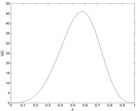
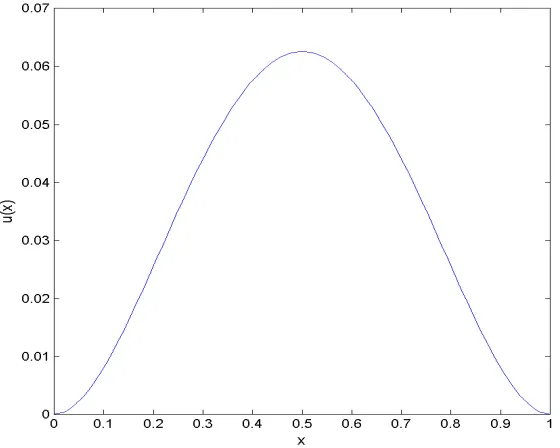
2.4.3 Direct Problem Numerical Examples . . . 58

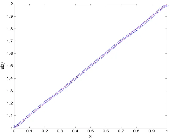
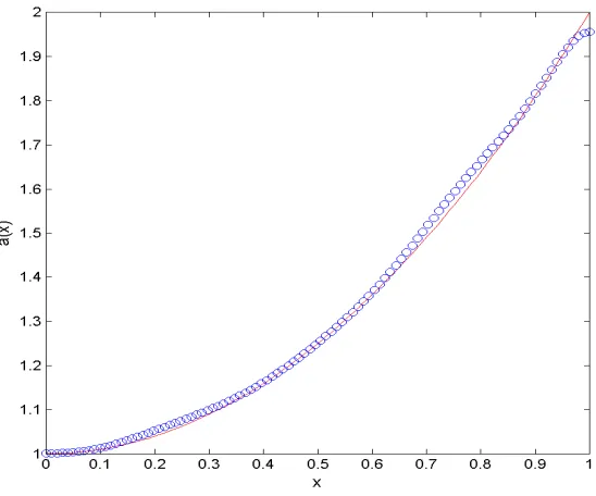
2.4.4 Inverse Problem Numerical Examples . . . 61

2.5 Modiﬁed Output Least-Squares Approach . . . 63

2.5.2 Gradient Derivation . . . 63

2.5.3 Direct Problem Numerical Examples . . . 64

2.6 Equation Error Approach . . . 69

2.6.1 Derivation of Cost Functional . . . 69

2.6.3 Cost Functional Gradient Derivation . . . 72

3 Parabolic Inverse Problem 75 3.1 Direct Problem Formulation . . . 76

3.2 FEM Matrix Computations . . . 79

3.3 Inverse Problem Formulation . . . 82

3.4 Derivative Computation . . . 85

3.4.1 The Fr´echet derivative of the parameter to solution operator . . . 85

3.4.2 Gˆateaux Derivative of the Parameter to Solution Operator . . . 87

3.4.3 Deriving the derivative of the OLS cost functional . . . 88

3.4.4 Completing the Gradient Computation . . . 90

3.4.5 Parabolic Cost Function Derivative Computation . . . 91

3.5 Numerical Examples . . . 94

3.5.1 Examples of 1-Dimensional Parabolic Direct Problem . . . 94

(8)

Section CONTENTS

3.5.3 Examples of 2-Dimensional Parabolic Direct Problem . . . 100

3.5.4 Examples of 2-Dimensional Parabolic Inverse Problem . . . 106

4 Appendix 109 4.1 Function Spaces . . . 109

4.2 The Fr´echet Derivative . . . 111

4.3 The Gˆateaux Derivative . . . 111

4.4 Bilinear and Trilinear Form and Properties . . . 111

4.5 Existence and Uniqueness Theorems . . . 114

4.6 The Adjoint Operator . . . 115

(9)

Introduction

There is a broad range of mathematical problems that can be classiﬁed under the title of inverse

problems. Their main overarching commonality is they involve converting a set of observations of

a system into information about the system’s unobservable properties. In this thesis we will be

concerned with systems that are described by a diﬀerential equation and the information we wish

to discover are coeﬃcients in the diﬀerential equation. We formulate the inverse problem by posing

a constrained optimization problem which minimizes a norm of the observation data by choosing

the optimal coeﬃcient.

This thesis implements multiple inverse problem formulations involving various cost functionals and

methods of calculating the gradient of the cost functionals. We implement the output least-squares,

modiﬁed output least-squares and equation error cost functionals. We explore inverse problems that

involve two separate diﬀerential equations: a fourth-order diﬀerential equation and parabolic partial

diﬀerential equation.

In the ﬁrst chapter we formally deﬁne the inverse problem and the direct problem in general terms,

deﬁne important concepts such as well-posedness, cost functionals, regularization parameters, and

discuss the algorithms for solving the inverse problem.

The Second chapter involves solving the inverse problem of identifying a variable coeﬃcient in

a fourth-order ordinary diﬀerential equation. We show the detailed derivation and solution method

(10)

Section CONTENTS

general derivation of the adjoint stiﬀness matrix which is used in the computation of the cost

functional’s gradient. Finally, we show the implementation details and show numerical examples

for output least-squares, modiﬁed output least-squares and equation error approach.

The third chapter outlines the methods and procedures for deriving and implementing methods

for finding a spatially varying coefficient in a general parabolic partial differential equation. We

compute the gradient of the output least-squares cost functional by an alternate method to the

adjoint stiﬀness approach and give numerical examples.

This thesis is meant to be self-contained, giving a complete derivation and explanation for all

concepts and methods used in solving the inverse problems. The last chapter is an appendix

containing deﬁnitions of concepts that might not be familiar to undergraduate and graduate

(11)

Chapter 1

Inverse Problem of Coefficient

Identification

1.1

Direct Problem and Inverse Problem

Inverse problems arise when our objective is to recover information about a system from observations

of the system. The system is usually closed which refers to the property that the information we

wish to recover cannot be directly observed.

The direct problem relates a set of model parameters to a solution of the system. The forward

operator, the operator deﬁning the direct problem, contains information about the relationship

between the model parameters determining what occurs inside the closed system and the measurement

of what we observe occurring outside the system. We deﬁne the forward operator as _F :_{A →}D

where _A is the set of model all possible parameters and D is the set of possible solutions or measurements. The forward problem is deﬁned as:

Find the solution d_∈D such that

(12)

Section 1.2. WELL-POSEDNESS

given a speciﬁca_{∈ A}.

Conversely, the inverse problem relates the observations outside the system, to model parameters.

In inverse problems we are provided with measurement data of our solution, and we are concerned

with identifying the correct model parameters. Thus, we can deﬁne the inverse problem as:

Find the model parameter a_{∈ A}such that

F(a) =d (1.2)

given a speciﬁcd_∈D.

In this paper we will consider models _F to be differential equations, parametersa are coefficients in the differential equations, anddis a possible solution to_F in the context of the forward problem (1.1) and a discrete set of measurement data in the context of the inverse problem (1.2).

The forward operator _F is a diﬀerential equation which can be discretized to a ﬁnite dimensional system of equations. Therefore the forward problem and inverse problem can be posed as satisfying

Fa=dwhere_F is anm_×n matrix, ais ann_×1 vector, anddis am_×1 vector.

1.2

Well-posedness

Inverse problems are often diﬃcult to solve because of the issue of ill-posedness [1]. Inverse problems

are often ill-posed because there is often more than one choice of coeﬃcientawhich allows_F(a) =d

to be satisﬁed. A problem is said to be ill-posed if it fails to be well-posed according the deﬁnition

provided by Jacques Hadamard in 1902.

A problem is well-posed in the sense of Hadamard if it has the properties that

(13)

Section 1.3. GENERAL INVERSE PROBLEM FORMULATION

ii The solution is unique.

iii The solution depends continuously on the data.

The last property, perhaps being the most important in ﬁnding the solution of an inverse problem,

may determine the stability of our solution. If the solution of the problem does not depend

continuously on the data then small changes in the data will result in large changes in our solution.

Therefore it will be diﬃcult to implement a numerical algorithm to approximate our solution. In

this case the problem must be reposed to satisfy the stability requirement. Note that this can be

achieved in several ways, one possible method is with the addition of a regularization term which

we will utilize in this paper.

1.3

General Inverse Problem Formulation

We present the inverse problem of identifying a(x) as a ﬁnite dimensional optimization problem. The solution to the problem is formulated as the minimizer of a cost functional which is deﬁned by

the coeﬃcient to solution mapping. The minimization problem has the following form:

min

a(x)∈AJ(a) (1.3)

whereJis a function from_AtoRcalled the cost functional and_Ais the set of admissible coeﬃcients. We want our solution to satisfy the inverse problem condition from the previous section that

F(a) =dwhere_F is a diﬀerential equation model, ais the parameter we wish to identify, anddis the given data. Therefore we can deﬁne the cost functional in the above minimization problem as

J(a) =_||F(a)₋z_||2 (1.4)

for some suitable norm, andz is the discrete set of measurement data.

Since the direct problem is a diﬀerential equation, we can reformulate it in its corresponding

variational form given by (1.5). Therefore the forward operator is replaced with the solutionu_{∈ V}

(14)

Section 1.4. REGULARIZATION

b(u, v) =f(v) _∀v_{∈ V} (1.5)

where b(_·,_·) is the bilinear form and _V is the typical space of test functions deﬁned in variational problems. The optimization approach for the inverse problem has the form

min

a(x)∈A||u(a)−z||

2 _(1.6)

whereu is the solution to the variational problem depending on the parameter a(x).

1.4

Regularization

The inverse problem of identifying a spatially varying coeﬃcient in a diﬀerential equation is

subject to problems of ill-posedness and overﬁtting. We introduce the process regularization which

introduced additional information in order to create a well-posed problem and prevent overﬁtting.

The issue of well-posedness was covered in previous sections. Overﬁtting occurs when the values

of the recovered coeﬃcient are inﬂuenced by noise instead of by the underlying model or data.

Regularization introduces a tradeoff between fitting the data with the correct coefficient and

reducing a norm of the coeﬃcient.

min

a(x)∈AJ(a) +ǫR(a) (1.7)

We redeﬁne the minimization problem by introducing the regularization functional, R(a), and the regularization parameter, ǫ. The regularization parameter is a small positive constant and can be deﬁned in alternate functional forms.

The coefficient we wish to identify is an element of a specific function space of admissible coefficients

deﬁned by

A=_{a=a(x)_|a_∈H1(Ω),0< k0≤a≤k1 <∞ on Ω, ki∈R+} (1.8)

(15)

Section 1.5. INVERSE PROBLEM ALGORITHM

L2-norm: _||a_||_H0_(Ω)=||a||_L2_(Ω)=

Z

Ω|

a_|2 (1.9)

H1-norm: _||a_||_H1_(Ω)=

Z

Ω|

a_|2+

Z

Ω|∇

a_|2 (1.10)

H1-seminorm: _||a_||H˜1(Ω) =

Z

Ω|∇

a_|2 (1.11)

where ˜H1(Ω) denotes the semi-norm ofH1(Ω).

1.5

Inverse Problem Algorithm

In this section we will brieﬂy discuss the inverse problem algorithm that will be implemented in

the following chapters. We provide general descriptions of how to solve an inverse problem of

identifying a coeﬃcient from observation data. The steps are as follows:

1. Initial guess for the coeﬃcient: (ai=a0). 2. Solve the direct problem: Findu(ai).

3. Evaluate cost functional value: J(ai).

4. Compute gradient of cost functional: _∇J(ai).

5. Using gradient descent algorithm, move in direction of steepest descent: Compute ai+1. 6. Repeat steps 2-6 until stopping criteria is satisﬁed: _||∇J(ai)||<tol.

First, an initial guess for the coeﬃcient is provided based on some assumptions of the data. A

reasonably good initial guess is required for convergence of the algorithm.

Second, we ﬁnd the solution of the direct problem from the appropriate diﬀerential equation using

the provided coeﬃcient.

Next, we use u(ai) from step 2 to compute the value of the cost functional and the gradient of

(16)

Section 1.5. INVERSE PROBLEM ALGORITHM

A constrained optimization method, such as a gradient descent algorithm is used to ﬁnd ai+1 which reduces the value of the cost functional. In our numerical examples we will use a conjugate

gradient trust region method which usesJ(ai) and ∇J(ai) to ﬁnd ai+1.

We repeat steps 2-6 until the necessary stopping criteria is met. In this case our stopping criteria

is the condition that the gradient of the cost functional_||∇Jai||is less than a pre-deﬁned tolerance

(17)

Chapter 2

The Fourth-Order Inverse Problem

In this section we study a general fourth-order diﬀerential equation with three spatially varying

coefficients. The case of identifying a coefficient in a fourth-order differential equation has an

important application in materials science; speciﬁcally in modeling the deﬂection of a beam.

This has been studied extensively in several contexts involving beam problems and the related

2-dimensional modeling of car windshields studied in [2] and [3].

2.1

Direct Problem Formulation

In this section we introduce the problem of solving a fourth-order diﬀerential equation by ﬁnite

element methods. The general partial diﬀerential equation is

d2 dx2

a(x)d 2_u dx2

− d

dx

b(x)du dx

+c(x)u=f(x), x_∈Ω (2.1)

u(x) = du

dx(x) = 0 ∀x∈Γ (2.2)

where f is a real-valued piecewise continuous and bounded function, Ω = [0,1] and Γ =_{0,1_}. In this problem we have homogeneous Dirichlet and Neumann boundary conditions. These are often

called ’clamped’ boundary conditions. We deﬁne the linear space of test functions as follows:

V =_{v_|v and dv

dx are continuous on Ω, and v(x) =

dv

(18)

Section 2.1. DIRECT PROBLEM FORMULATION

We introduce the following inner product notation to be used throughout the thesis which applies

to real-valued piecewise continuous and bounded functions.

(v, w) =

Z

Ω

v(x)w(x)dx

Next we obtain the weak form, or variational form, of the fourth-order diﬀerential equation by

distributing test functionvthrough equation (2.1), integrating over Ω, and applying integration by parts with boundary conditions deﬁned by (2.2) and (2.3).

Z

Ω d2 dx2

a(x)d 2_u dx2

vdx₋

Z

Ω d dx

b(x)du dx

vdx+

Z

Ω

c(x)uvdx=

Z

Ω

f(x)vdx

=_⇒ d

dx

a(x)d 2_u dx2

v Γ − Z Ω d dx

a(x)d 2_u dx2

dv

dxdx −b(x)du

dxv

Γ + Z Ω

b(x)du dx

dv

dxdx+

Z

Ω

c(x)uvdx=

Z

Ω

f(x)vdx

=_⇒ d

dx

a(x)d 2_u dx2

v Γ

−a(x)d 2_u dx2

dv dx Γ + Z Ω

a(x)d 2_u dx2

d2v

dx2dx

−b(x)du dxv

Γ + Z Ω

b(x)du dx

dv

dxdx+

Z

Ω

c(x)uvdx=

Z

Ω

f(x)vdx

Using boundary conditions supplied by (2.3) the ﬁrst two terms of the above equation evaluate to

0. Therefore we have the following equation which we can also write in variational form. Note that

this is true for every test function sincev was chosen arbitrarily from the linear space.

Z

Ω

a(x)d 2_u dx2

d2v

dx2dx+

Z

Ω

b(x)du dx

dv

dxdx+

Z

Ω

c(x)uvdx=

Z

Ω

f(x)vdx _∀v_{∈ V}

=_⇒

a(x)d 2_u dx2,

d2_v dx2

+

b(x)du dx,

dv

dx

+ (c(x)u, v) = (f(x), v) _∀v_{∈ V}

We define _Vh to be a finite dimensional subspace of V, which is an infinite dimensional space

of functions, in order to properly deﬁne the ﬁnite element discretization of our solution. In the

following section we will formally deﬁne the corresponding basis functions, matrices, and ﬁnite

(19)

Section 2.2. FEM IMPLEMENTATION

2.2

FEM Implementation

2.2.1 Stiffness Matrix Computation

The solution, u, has a unique representation given a basis function representation. The basis function representation is

u=

n

X

j=1

[ujφj+ ˆujψj]. (2.4)

whereuj represents the coefficients on φj and ûj represents the coefficients onψj.

Substituting the basis function representation of our solution into the weak form equation allows us

to put the equation in a form where we can calculate the adjoint stiﬀness matrix. First we replace

the test functionv, with each of the basis functions and obtain the following two equations.



a(x)

n

X

j=1

ujφ′′j + ˆujψ′′j

, φ′′_i



+



b(x)

n

X

j=1

ujφ′j+ ˆujψ′j

, φ′_i





+



c(x)

n

X

j=1

ujφ′j+ ˆujψj, φi



= (fi, φi) (2.5)



a(x)

n

X

j=1

ujφ′′j + ˆujψj′′

, ψ′′_i



+



b(x)

n

X

j=1

ujφ′j + ˆujψ′j

, ψ_i′





+



c(x)

n

X

j=1

ujφ′j+ ˆujψj, ψi



= (fi, ψi) (2.6)

where φ′′ _{is the derivative} d2_φ

dx2 and likewise with ψ. We introduce the notation that Φ = [φ, ψ]′,

where′ is the transpose operation, so the above two equations condense to the following equation.

n

X

j=1

ujAk akφ′′j,Φ′′i

+

n

X

j=1

u′_jAk akψ′′j,Φ′′i

+

n

X

j=1

ujBk bkφ′j,Φ′i

+

n

X

j=1

u′_jBk bkψ′j,Φ′i

+

n

X

j=1

ujCk(ckφj,Φi) + n

X

j=1

u′_jCk(ckψjΦi) = (fi,Φi) (2.7)

where we have made a substitution for the coeﬃcients in terms of their basis functions by the

(20)

a(x) =

n

X

k=1

Akak,

b(x) =

n

X

k=1

Bkbk, and

c(x) =

n

X

k=1

Ckck.

Ak,Bk, and Ck represent the kth coeﬃcient andak,bk, and ck represent thekth basis function for

the corresponding coeﬃcient. Imposing basis function conditions we can solve for the precise cubic

polynomials representing the solution.

φj(x) =

        

1

h3

h

−2x3+ 3(xj−1+xj)x2−6xj−1xjx+ (3xj−xj−1)x2j−1

i

:x_∈Ij

1

h3

h

2x3₋3(xj+xj+1)x2+ 6xjxj+1x−(3xj −xj+1)x2j+1

i

:x_∈Ij+1

0 :otherwise

ψj(x) =

        

1

h2

h

x3₋₍₂_x

j−1+xj)x2+ (xj−1+ 2xj)xj−1x−x2j−1xj

i

:x_∈Ij

1

h2

h

x3₋₍_x

j+ 2xj+1)x2+ (2xj +xj+1)xj+1x−xjx2j+1

i

:x_∈Ij+1

0 :otherwise

whereIj is the interval to the left ofxj deﬁned as Ij = [xj−1, xj] and similarly Ij+1= [xj, xj+1].

The following values are calculated by taking the appropriate derivative and ﬁnding the basis

function value at the speciﬁed point. We also impose the condition that we have a regular mesh

(i.e. we have equally spaces nodes over the mesh). These values are necessary for the computation

of the stiﬀness matrix.

φj(xj+1) = 0

φj(xj−1) = 0

φj(xj+1/2) = 1/2

φj(xj−1/2) = 1/2

φj(xj) = 1

φ′_j(xj+1) = 0

φ′_j(xj−1) = 0

φ′_j(xj+1/2) =−₂3_h

φ′

j(xj−1/2) = 23h

(21)

φ′′_j(xj+1) = _h62

φ′′_j(xj−1) = _h62

φ′′_j(x_j₊₁_/₂) = 0

φ′′_j(x_j−₁_/₂) = 0

φ′′_j(xj) =−_h62

ψj(xj+1) = 0

ψj(xj−1) = 0

ψj(xj+1/2) =h/8

ψj(xj−1/2) =−h/8

ψj(xj) = 0

ψ′

j(xj+1) = 0

ψ′

j(xj−1) = 0

ψ′

j(xj+1/2) =−14

ψ′

j(xj−1/2) =−14

ψ_j′(xj) = 1

ψ_j′′(xj+1) = 2_h

ψ_j′′(xj−1) =−2_h

ψ_j′′(xj+1/2) =−_h1

ψ_j′′(xj−1/2) = 1h

lim_x→x−

j ψ

′′

j(xj) = _h4

lim_x→x+

j ψ

′′

j(xj) =−4_h

In the following equations we will derive the values for each entry in the submatricesA,B,C, and

D. They will be used to construct the stiﬀness matrix K as a block matrix.

Ai,j =

a(x)φ′′_j, φ′′_i Bi,j =

a(x)ψ′′_j, φ′′_i Ci,j =

b(x)φ′_j, φ′_i Di,j =

b(x)ψ_j′, φ′_i Ei,j = (c(x)φj, φi)

Fi,j = (c(x)ψj, φi)

Gi,j =

a(x)φ′′_j, ψ_i′′ Hi,j =

a(x)ψ_j′′, ψ_i′′ Ii,j =

b(x)φ′_j, ψ′_i Ji,j =

b(x)ψ_j′, ψ′_i Ki,j = (c(x)φj, ψi)

(22)

K =



 A+C+E B+D+F

G+I+K H+J +L



 U =



 u

ˆ

u



 F =



 Fφ

Fψ



 (2.8)

⇒K(A)U =F (2.9)

Note that matrices A, C, E, H, J, and L are symmetric. AlsoG =BT,I =DT, and K = FT. Next submatrix of the stiﬀness matrix, K, is calculated.

Aj,j = a(x)φ′′j, φ′′j

=

Z xj+1

xj−1

a(x)(φ′′_j)2dx

=

Z xj

xj−1

a(x)(φ′′_j)2dx+

Z xj+1

xj

a(x)(φ′′_j)2dx ≈ h₆aj−1φ′′j(xj−1)2+ 4aj−1

2φ ′′ j(xj−1

2)

2₊_a

jφ′′j(xj)2

+h

6

ajφ′′j(xj)2+ 4a_j₊1 2φ

′′ j(xj+1

2)

2₊_a

j+1φ′′j(xj+1)2

= h

6

aj−1

36

h4

+ 0 +aj

36 h4 +h 6 aj 36 h4

+ 0 +aj+1

36

h4

= 6

h3 (aj−1+ 2aj+aj+1)

Aj−1,j = a(x)φ′′j, φ′′j−1

=

Z xj

xj−1

a(x)φ′′_j−₁φ′′_jdx

≈ h₆aj−1φ′′j−1(xj−1)φ′′j(xj−1) + 4a_j−1 2φ

′′

j−1(xj−1 2)φ

′′ j(xj−1

2) +ajφ ′′

j−1(xj)φ′′j(xj)

= h

6

aj−1

−36

h4

+ 0 +aj

−36

h4

= 6

h3 (−aj−1−aj)

Aj,j−1=Aj−1,j

Bj,j = a(x)ψj′′, φ′′j

=

Z xj+1

xj−1

(23)

=

Z xj

xj−1

a(x)ψ_j′′φ′′_j dx+

Z xj+1

xj

a(x)ψ_j′′φ′′_j dx ≈ h₆aj−1ψj′′(xj−1)φ′′j(xj−1) + 4a_j−1

2ψ ′′ j(xj−1

2)φ ′′ j(xj−1

2) +ajψ ′′

j(xj)φ′′j(xj)

+ h

6

ajψj′′(xj)φ′′j(xj) + 4aj−1 2ψ

′′ j(xj+1

2)φ ′′ j(xj+1

2) +ajψ ′′

j(xj+1)φ′′j(xj+1)

= h

6

aj−1

−12

h3

+ 0 +aj

−24 h3 +h 6 aj 24 h3

+ 0 +aj

12

h3

= 2

h2(−aj−1+aj+1)

Bj−1,j= a(x)ψj′′, φ′′j−1

=

Z xj

xj−1

a(x)ψ_j′′φ′′_j−₁dx

≈ h₆aj−1ψ′′j(xj−1)φ′′j−1(xj−1) + 4aj−1 2ψ

′′ j(xj−1

2)φ ′′

j−1(xj−1

2) +ajψ ′′

j(xj)φ′′j−1(xj)

= h

6

aj−1

12

h3

+ 0 +aj

24

h3

= 2

h2(aj−1+ 2aj)

Bj,j−1= a(x)ψj−′′ 1, φ′′j

=

Z xj

xj−1

a(x)ψ′′_j−₁φ′′_j dx

≈ h₆aj−1ψj−′′ 1(xj−1)φ′′j(xj−1) + 4a_j−1 2ψ

′′

j−1(xj−1 2)φ

′′ j(xj−1

2) +ajψ ′′

j−1(xj)φ′′j(xj)

= h

6

aj−1

−24

h3

+ 0 +aj

−12

h3

= 2

h2 (−2aj−1−aj)

Hj,j= a(x)ψj′′, ψ′′j

=

Z xj+1

xj−1

a(x)(ψ′′_j)2dx

=

Z xj

xj−1

a(x)(ψ′′_j)2dx+

Z xj+1

xj

a(x)(ψ_j′′)2dx ≈ h₆aj−1ψj′′(xj−1)2+ 4a_j−1

2ψ ′′ j(xj−1

2)

2₊_a

jψj′′(xj)2

+h

6

ajψj′′(xj)2+ 4aj+1 2ψ

′′ j(xj+1

2)

2₊_a

j+1ψj′′(xj+1)2

(24)

= h

6

aj−1

4

h2

+ 4a_j−1 2

1

h2

+aj

16 h2 +h 6 aj 16 h2

+ 4a_j₊1 2

1

h2

+aj+1

4

h2

≈ ₃2_h kj−1+k_j−1

2 + 8kj +kj+ 1

2 +kj+1

= 1

h(kj−1+ 6kj+kj+1) Hj−1,j= a(x)ψj′′, ψ′′j−1

=

Z xj

xj−1

a(x)ψ′′_j−₁ψ_j′′dx

≈ h₆aj−1ψj−′′ 1(xj−1)ψj′′(xj−1) + 4a_j−1 2ψ

′′

j−1(xj−1 2)ψ

′′ j(xj−1

2) +ajψ ′′

j−1(xj)ψj′′(xj)

= h

6

aj−1

8

h2

+ 4a_j−1 2

−1

h2

+aj

8 h2 = 1 h

aj−1 8

h2 + (aj−1+aj)

−2

h2 +aj 8

h2

= 1

h(aj−1+aj) Hj,j−1 =Hj−1,j

Cj,j = b(x)φ′j, φ′j

=

Z xj+1

xj−1

b(x)(φ′_j)2dx

=

Z xj

xj−1

b(x)(φ′_j)2dx+

Z xj+1

xj

b(x)(φ′_j)2dx ≈ h

6

bj−1φ′j(xj−1)2+ 4b_j−1 2φ

′ j(xj−1

2)

2₊_b

jφ′j(xj)2

+h

6

bjφ′j(xj)2+ 4bj+1 2φ

′ j(xj+1

2)

2₊_b

j+1φ′j(xj+1)2

= h

6

0 + 4b_j−1 2

9 4h2

+ 0 + h 6

0 + 4b_j₊1 2

9 4h2

+ 0 = 3 2h

b_j−1 2 +bj+

1 2

≈ ₄3_h(bj−1+ 2bj+bj+1)

Cj−1,j= b(x)φ′j, φ′j−1

=

Z xj+1

xj−1

(25)

=

Z xj

xj−1

b(x)φ′_j−₁φ′_jdx+

Z xj+1

xj

b(x)φ′_j−₁φ′_jdx ≈ h₆bj−1φ′j−1(xj−1)φ′j(xj−1) + 4b_j−1

2φ ′

j−1(xj−1 2)φ

′ j(xj−1

2) +bjφ ′

j−1(xj)φ′j(xj)

= h

6

0 + 4b_j−1 2

−9 4h2

+ 0

= −3 2h

b_j−1 2

≈ −₄_h3(bj−1+bj)

Cj,j−1 =Cj−1,j

Dj,j = b(x)ψ′j, φ′j

=

Z xj+1

xj−1

b(x)ψ_j′φ′_jdx

=

Z xj

xj−1

b(x)ψ′_jφ′_jdx+

Z xj+1

xj

b(x)ψ_j′φ′_jdx ≈ h₆bj−1ψj′(xj−1)φ′j(xj−1) + 4bj−1

2ψ ′ j(xj−1

2)φ ′ j(xj−1

2) +bjψ ′

j(xj)φ′j(xj)

+h

6

bjψ′j(xj)φ′j(xj) + 4b_j₊1 2ψ

′ j(xj+1

2)φ ′ j(xj+1

2) +bj+1ψ ′

j(xj+1)φ′j(xj+1)

= h

6

0 + 4b_j−1 2 −1 4 3 2h + 0 +h 6

0 + 4b_j₊1 2 −1 4 −3 2h + 0 = 1 4

−b_j−1 2 +bj+

1 2

≈ 1₈(₋bj−1+bj+1)

Dj−1,j= b(x)ψ′j, φ′j−1

=

Z xj+1

xj−1

b(x)ψ′_jφ′_j−₁dx

=

Z xj

xj−1

b(x)ψ′_jφ′_j−₁dx+

Z xj+1

xj

b(x)ψ′_jφ′_j−₁dx ≈ h

6

bj−1ψ′j(xj−1)φ′j−1(xj−1) + 4b_j−1 2ψ

′ j(xj−1

2)φ ′

j−1(xj−1

2) +bjψ ′

j(xj)φ′j−1(xj)

= h

6

0 + 4b_j−1 2 −1 4 −3 2h + 0 = 1 4

b_j−1 2

(26)

≈ 1₈(bj−1+bj)

Dj,j−1 = b(x)ψ′j−1, φ′j

=

Z xj+1

xj−1

b(x)ψ_j−′ ₁φ′_jdx

=

Z xj

xj−1

b(x)ψ_j−′ ₁φ′_jdx+

Z xj+1

xj

b(x)ψ′_j−₁φ′_jdx ≈ h

6

bj−1ψ′j−1(xj−1)φ′j(xj−1) + 4b_j−1 2

ψ_j−′ ₁(x_j−1 2

)φ′_j(x_j−1 2

) +bjψ′j−1(xj)φ′j(xj)

= h

6

0 + 4b_j−1 2 −1 4 3 2h + 0

= −1 4

b_j−1 2

≈ −1

8 (bj−1+bj)

Jj,j = b(x)ψj′, ψ′j

=

Z xj+1

xj−1

b(x)(ψ′_j)2dx

=

Z xj

xj−1

b(x)(ψ′_j)2dx+

Z xj+1

xj

b(x)(ψ′_j)2dx ≈ h₆ bj−1ψj′(xj−1)2+ 4b_j−1

2ψ ′ j(xj−1

2)

2₊_b

jψ′j(xj)2

+h

6

bjψj′(xj)2+ 4b_j₊1 2ψ

′ j(xj+1

2)

2₊_b

j+1ψ′j(xj+1)2

= h

6

0 + 4b_j−1 2

1 16

+bj

+h

6

bj+ 4b_j₊1 2 1 16 + 0 = h 24

b_j−1

2 + 8bj +bj+ 1 2

≈ ₄₈h (bj−1+ 18bj +bj+1)

Jj−1,j = b(x)ψj′, ψ′j−1

=

Z xj+1

xj−1

b(x)ψ_j−′ ₁ψ′_jdx

=

Z xj

xj−1

b(x)ψ_j−′ ₁ψ′_jdx+

Z xj+1

xj

b(x)ψ_j−′ ₁ψ′_jdx ≈ h₆ bj−1ψj−′ 1(xj−1)ψj′(xj−1) + 4bj−1

2ψ ′

j−1(xj−1 2)ψ

′ j(xj−1

2) +bjψ ′

j−1(xj)ψ′j(xj)

(27)

= h

6

0 + 4b_j−1 2 1 16 + 0 = h 24

b_j−1 2

≈ ₄₈h (bj−1+bj)

Jj,j−1=Jj−1,j

Ej,j = (c(x)φj, φj)

=

Z xj+1

xj−1

c(x)(φj)2dx

=

Z xj

xj−1

c(x)(φj)2dx+

Z xj+1

xj

c(x)(φj)2dx

≈ h₆ cj−1φj(xj−1)2+ 4c_j−1

2φj(xj− 1 2)

2₊_c

jφj(xj)2

+h

6

cjφj(xj)2+ 4cj+1 2φj(xj+

1 2)

2₊_c

j+1φj(xj+1)2

= h

6

0 + 4c_j−1 2

1 4

+cj

+h

6

cj+ 4c_j₊1 2 1 4 + 0 = h 6

c_j−1

2 + 2cj +cj+ 1 2

≈ ₁₂h (cj−1+ 6cj +cj+1)

Ej−1,j = (c(x)φj, φj−1) =

Z xj+1

xj−1

c(x)φj−1φjdx

=

Z xj

xj−1

c(x)φj−1φjdx+

Z xj+1

xj

c(x)φj−1φjdx

≈ h₆ cj−1φj−1(xj−1)φj(xj−1) + 4cj−1

2φj−1(xj− 1

2)φj(xj− 1

2) +cjφj−1(xj)φj(xj)

= h

6

0 + 4c_j−1 2 1 4 + 0 = h 6

c_j−1 2

≈ h

12(cj−1+cj)

(28)

Fj,j = (c(x)ψj, φj)

=

Z xj+1

xj−1

c(x)ψjφjdx

=

Z xj

xj−1

c(x)ψjφjdx+

Z xj+1

xj

c(x)ψjφjdx

≈ h₆cj−1ψj(xj−1)φj(xj−1) + 4cj−1

2ψj(xj− 1

2)φj(xj− 1

2) +cjψj(xj)φj(xj)

+h

6

cjψj(xj)φj(xj) + 4c_j₊1

2ψj(xj+ 1

2)φj(xj+ 1

2) +cj+1ψj(xj+1)φj(xj+1)

= h

6

0 + 4c_j−1 2 −h 8 1 2 + 0 + h 6

0 + 4c_j₊1 2 h 8 1 2 + 0 = h 2 24

−c_j−1 2 +cj+

1 2

≈ h

2

48(−cj−1+cj+1)

Fj−1,j= (c(x)ψj, φj−1) =

Z xj+1

xj−1

c(x)ψjφj−1dx =

Z xj

xj−1

c(x)ψjφj−1dx+

Z xj+1

xj

c(x)ψjφj−1dx

≈ h₆cj−1ψj(xj−1)φj−1(xj−1) + 4cj−1

2ψj(xj− 1

2)φj−1(xj− 1

2) +cjψj(xj)φj−1(xj)

= h

6

0 + 4c_j−1 2 −h 8 1 2 + 0

= −h 2

24

c_j−1 2

≈ −h

2

48 (cj−1+cj)

Fj,j−1= (c(x)ψj−1, φj)

=

Z xj+1

xj−1

c(x)ψj−1φjdx

=

Z xj

xj−1

c(x)ψj−1φjdx+

Z xj+1

xj

c(x)ψj−1φjdx

≈ h₆ cj−1ψj−1(xj−1)φj(xj−1) + 4cj−1

2ψj−1(xj− 1

2)φj(xj− 1

2) +cjψj−1(xj)φj(xj)

= h

6

(29)

= h

2

24

c_j−1 2

≈ h

2

48(cj−1+cj)

Lj,j = (c(x)ψj, ψj)

=

Z xj+1

xj−1

c(x)(ψj)2dx

=

Z xj

xj−1

c(x)(ψj)2dx+

Z xj+1

xj

c(x)(ψj)2dx

≈ h

6

cj−1ψj(xj−1)2+ 4c_j−1 2

ψj(x_j−1 2

)2+cjψj(xj)2

+h

6

cjψj(xj)2+ 4cj+1

2ψj(xj+ 1 2)

2₊_c

j+1ψj(xj+1)2

= h

6

0 + 4c_j−1 2 h2 64 + 0 +h 6

0 + 4c_j₊1 2 h2 64 + 0 = h 3 96

c_j−1 2 +cj+

1 2 ≈ h 3 192

cj−1+ 2cj+

64

h2cj+cj+1

Lj−1,j = (c(x)ψj, ψj−1) =

Z xj+1

xj−1

c(x)ψj−1ψjdx

=

Z xj

xj−1

c(x)ψj−1ψjdx+

Z xj+1

xj

c(x)ψj−1ψjdx

≈ h₆cj−1ψj−1(xj−1)ψj(xj−1) + 4cj−1

2ψj−1(xj− 1

2)ψj(xj− 1

2) +cjψj−1(xj)ψj(xj)

= h

6

0 + 4c_j−1 2

−h2

64

+ 0

= −h 3

96

c_j−1 2

≈ −h

3

192 (cj−1+cj)

(30)

2.2.2 Load Vector Computation

In this section we compute the fourth order load vector which is constructed byF = (Fφ, Fψ) where

Fφ= (f, φj)j=1,2,...,n and Fφ= (f, ψj)j=1,2,...,n. In the following derivations we use the deﬁnition of

the load vector and numerically approximate the integrals with Simpson’s rule.

(Fφ)_j =

Z 1

0

f φjdx

=

Z xj

xj−1

f φjdx+

Z xj+1

xj

f φjdx

=hj 6

f(xj−1)φj(xj−1) + 4f(xj−1/2)φj(xj−1/2) +f(xj)φj(xj)

+hj+1 6

f(xj)φj(xj) + 4f(xj+1/2)φj(xj+1/2) +f(xj+1)φj(xj+1)

=hj 6

2f(x_j−₁_/₂) +f(xj)

+hj+1 6

f(xj) + 2f(xj+1/2)

If the mesh is sufficiently fine (i.e. nis sufficiently large) then we can approximate f(x_j−₁_/₂) and

f(x_j₊₁_/₂) by f(xj).

=1 3

hjf(xj−1/2) +

hj +hj+1

2 f(xj) +hj+1f(xj+1/2)

=

hj+hj+1 2

f(xj)

(Fψ)_j =

Z 1

0

f ψjdx

=

Z xj

xj−1

f ψjdx+

Z xj+1

xj

f ψjdx

=hj 6

f(xj−1)ψj(xj−1) + 4f(xj−1/2)ψj(xj−1/2) +f(xj)ψj(xj)

+hj+1 6

f(xj)ψj(xj) + 4f(xj+1/2)ψj(xj+1/2) +f(xj+1)ψj(xj+1)

=₋h

2

j

12f(xj−1/2) +hj+1hjf(xj+1/2) =hj

12

−hjf(xj−1/2) +hj+1f(xj+1/2)

(31)

2.2.3 Mass Matrix Computation

In this section we derive the fourth-order mass matrix used in computation of cost functionals

and the gradient of cost functionals. The calculation requires much algebra so many steps are

omitted for to keep the explanation concise. The integrals in this section are computed exactly by

integrating and substitutingxj−1 =xj −h or xj+1 =xj+h.

M =



 A B

BT _C



 (2.10)

Ai,j =

Z 1

0

φiφjdx

Aj,j =

Z 1

0

φjφjdx

=

Z xj

xj−1

φ2_jdx+

Z xj+1

xj

φ2_jdx

=13 35

h7

h6 + 13 35

h7

h6 =26

35h

Aj−1,j =

Z 1

0

φj−1φjdx

=

Z xj

xj−1

φjφj−1dx =9

70h

Aj,j−1=Aj−1,j

Bi,j =

Z 1

0

φiψjdx

Bj,j =

Z 1

0

φjψjdx

=

Z xj

xj−1

φjψjdx+

Z xj+1

xj

φjψjdx

(32)

Section 2.3. INVERSE PROBLEM FORMULATION

Bj−1,j=

Z 1

0

φj−1ψjdx

=

Z xj

xj−1

φj−1ψjdx

=−13 420h

2

Bj,j−1=

Z 1

0

φjψj−1dx =

Z xj

xj−1

φjψj−1dx = 13

420h 2

Ci,j =

Z 1

0

ψiψjdx

Cj,j=

Z 1

0

ψjψjdx

=

Z xj

xj−1

ψ_j2dx+

Z xj+1

xj

ψ2_jdx

= 1

105

h7

h4 + 1 105

h7

h4

= 2

105

h7

h4

Cj−1,j=

Z 1

0

ψj−1ψjdx

=

Z xj

xj−1

ψjψj−1dx =−1

140h 3

Cj,j−1 =Cj−1,j

2.3

Inverse Problem Formulation

We introduce a modiﬁcation of the standard fourth order inverse problem. The problem becomes

(33)

d2 dx2

a(x)d 2_u₍_x₎

dx2

− d

dx

b(x)du(x) dx

+c(x)u(x) =f(x) (2.11) where the problem is deﬁned on the domain Ω = [0,1].

The weak form of the diﬀerential equation is obtained as in the previous section by integrating

by parts twice and applying boundary conditions. We ﬁnd the variational form to be

a(x)d 2_u dx2,

d2v

dx2

+

b(x)du dx,

dv

dx

+ (c(x)u, v) = (f, v) _∀v_{∈ V}. (2.12) After we obtain the solution to the direct problem, which was formulated above, we move on to

ﬁnding a fourth-order discretization of the necessary matrices and elements to minimize the cost

functional.

2.3.1 The Fr´echet derivative of the parameter to solution operator for fourth-order

equations

The parameter to solution mapping is deﬁned as F : _{A → V} where the solution belongs to _V, a Hilbert space, and the parameter belongs to _A, a Banach space.

The trilinear form comes from the variational form of the problem deﬁned in (2.12). We adopt the

notation that q= (a(x), b(x), c(x)). So given that the trilinear form is deﬁned as

T(q, u, v) :=

a(x)d 2_u dx2,

d2v

dx2

+

b(x)du dx,

dv

dx

+ (c(x)u, v) (2.13)

then we have

T(q, u, v) = (f, v) _∀v_{∈ V}. (2.14) We find the Fréchet Derivative of the parameter to solution mapping. Letq _∈int(_A) and δq be a perturbation on q such that q+δq _{∈ A}. Also define δw =F(q+δq)₋F(q) and u=F(q). Note that we can writeF(q+δq) asu+δw.

The variational form at q has the form

(34)

and the variational form atq+δq has the form

T(q+δq, u+δw, v) = (f, v) _∀v_{∈ V} (2.16) Next, we subtract (2.16) from (2.15) and simplify.

T(q, u, v)₋T(q+δq, u+δw, v) = 0

T(q, u, v)₋T(q, u+δw, v)₋T(δq, u+δw, v) = 0

T(q, u, v)₋T(q, u+δw, v)₋T(δq, u, v)₋T(δq, δw, v) = 0

T(q, u+δw, v) =T(q, u, v)₋T(δq, u, v)₋T(δq, δw, v)

Note that the last equation is in the form of the Fr´echet Derivative (4.10) which suggests the form

of the derivative DF(q). We see that the derivative of our solution isδu=DF(q)δq and is found by solving the variational equation

T(q, δu, v) =₋T(δq, u, v) _∀v_{∈ V}. (2.17) Note that the validity of this argument is not proved here. For a rigorous proof and derivation of

this we refer to [4]. For the particular problem we are considering this result translates into the

following equation.

ad

2_δu dx2 ,

d2_v dx2

+

bdδu

dx ,

dv

dx

+ (cδu, v) =

δad

2_u dx2,

d2_v dx2

+

δbdu

dx,

dv

dx

+ (δcu, v) (2.18)

2.3.2 Derivative of U(A)

The matrix U(A) is the solution to direct problem discretized by ﬁnite element method. We ﬁnd

δU in order to complete the calculation of the derivative of J(A) in the following sections. We begin with the direct problem

K(A)U =F. (2.19)

Next, we take the derivative of the above matrix equation. Utilizing chain rule and product rule

(35)

(DK(A)δA)U+K(A)δU = 0. (2.20)

We use the linearity of K(A) to simplify the expression and obtain an expression forδU.

(DK(A)δA)U +K(A)δU = 0 (2.21)

=_⇒K(A)δU =₋DK(A)(δA)U

=_⇒K(A)δU =₋K(δA)U

=_⇒δU =₋K(A)−1K(δA)U

(2.22)

2.3.3 Adjoint Stiffness Derivation

Here we derive the fourth-order adjoint stiﬀness matrix in general form from the deﬁnition of the

stiﬀness matrix. As before we use cubic basis functions for the solution space and piecewise linear

basis functions for the coefficient space. By definition of the the finite dimensional subspace of

linear test functions we see that v_∈Vh has the form

v=

n

X

j=1

vjΦj +v′jΨj (2.23)

and we impose the condition that the coeﬃcients have the form

a(x) =

m

X

k=1

Akak,b(x) = m

X

k=1

Bkbk andc(x) = m

X

k=1

Ckck. (2.24)

where wem=n+ 2. Also, note that ak, bk and ck are thekth basis functions andAk,Bk and Ck

are coeﬃcients on thekth _{basis functions for} _a₍_x_), _b₍_x_{) and}_c₍_x_{) respectively. Moreover, we adopt}

the notation that A = [Ak], B = [Bk] and C = [Ck] for k = 1,2, . . . m. We create a coeﬃcient

vector from these coeﬃcients given as

Q=

    

A B C

   

 (2.25)

(36)

[K(Q)]_ij =

Z

Ω

a(x) ¯Φ′′_jΦ¯′′_idx+

Z

Ω

b(x) ¯Φ′_jΦ¯′_idx+

Z

Ω

c(x) ¯ΦjΦ¯idx (2.26)

= Z Ω m X k=1

Akak

!

¯

Φ′′_jΦ¯′′_idx+

m

X

k=1

Bkbk

!

¯

Φ′_jΦ¯′_idx+

m

X

k=1

Ckck

!

¯ ΦjΦ¯idx

= m X k=1 Z Ω

akΦ¯′′jΦ¯′′idxAk+

Z

Ω

bkΦ¯′jΦ¯′idxBk+

Z

Ω

ckΦ¯jΦ¯idxCk

h

K(Q) ˜Vi

i= n X j=1 m X k=1 Z Ω

akΦ¯′′jΦ¯′′idxAk+

Z

Ω

bkΦ¯′jΦ¯′idxBk+

Z

Ω

ckΦ¯jΦ¯idxCk

!

˜

Vj (2.27)

= m X k=1 n X j=1 Z Ω

akΦ¯′′jΦ¯′′idxAkV˜j +

Z

Ω

bkΦ¯′jΦ¯′idxBkV˜j+

Z

Ω

ckΦ¯jΦ¯idxCkV˜j

We adopt the notation that ˜V =h V V′ iT _and

Tijk=

Z

Ω

akΦ¯′′jΦ¯′′idx+

Z

Ω

bkΦ¯′jΦ¯′idx+

Z

Ω

ckΦ¯jΦ¯idx. (2.28)

Furthermore,

h

K(Q) ˜Vi

i = n X j=1 m X k=1

TijkQk

!

˜

Vj = m X k=1   n X j=1

TijkV˜j



Qk=

h

L( ˜V)Qi

i (2.29)

The matrixL=L( ˜V) is known as the adjoint stiﬀness matrix. We have shown that it must follow the condition that

L( ˜V)Q=K(Q) ˜V , _∀A_∈Rm, _∀V˜ _∈R2n. (2.30) Furthermore, we shown the exact form of the adjoint stiﬀness matrix.

h L( ˜V)i

ik=

2n

X

j=1

TijkV˜j (2.31)

= 2n X j=1 Z Ω

akΦ¯′′jΦ¯′′idx+

Z

Ω

bkΦ¯′jΦ¯′idx+

Z

Ω

ckΦ¯jΦ¯idx

˜ Vj = n X j=1 Z Ω

akΦ′′jΦ¯′′idx+

Z

Ω

bkΦ′jΦ¯′idx+

Z

Ω

ckΦjΦ¯idx

Vj + 2n X j=1 Z Ω

akΨ′′jΦ¯′′idx+

Z

Ω

bkΨ′jΦ¯′idx+

Z

Ω

ckΨjΦ¯idx

V_j′

(37)

2.3.4 Adjoint Stiffness Matrix Computation

In this section we construct the adjoint stiffness matrix L by first creating submatrices A,B, C, and D (which are different from the A,B,C, and D in the previous section). These are used to create theL in the following manner.

Ai,k= n

X

j=1

Z 1

0

akφ′′jφ′′i dx

Vj

Bi,k= n

X

j=1

Z 1

0

akψj′′φ′′i dx

V_j′

Ci,k= n

X

j=1

Z 1

0

bkφ′jφ′idx

Vj

Di,k = n

X

j=1

Z 1

0

bkψ′jφ′idx

V_j′

Ei,k= n

X

j=1

Z 1

0

ckφjφidx

Vj

Fi,k= n

X

j=1

Z 1

0

ckψjφidx

V_j′

Gi,k= n

X

j=1

Z 1

0

akφ′′jψ′′i dx

Vj

Hi,k= n

X

j=1

Z 1

0

akψj′′ψi′′dx

V_j′

Ii,k= n

X

j=1

Z 1

0

bkφ′jψi′dx

Vj

Ji,k = n

X

j=1

Z 1

0

bkψj′ψi′dx

V_j′

Ki,k= n

X

j=1

Z 1

0

ckφjψidx

Vj

Li,k= n

X

j=1

Z 1

0

ckψjψidx

V_j′

L=



 A+B C+D E+F

G+H I+J K+L





⇒L(U)Q=K(Q)U

We construct the submatrices ofLby deriving each term of the matrices. We proceed by identifying

the intervals of compact support on which we integrate, we numerically approximate the individual

integrals by applying Simpson’s rule.

Ai,k= n

X

j=1

Z 1

0

akφ′′jφ′′i dx

Vj

A1,0 =

n

X

j=1

Z 1

0

a0φ′′jφ′′1dx

(38)

=

Z 1

0

a0(φ′′1)2dx

V1 =

Z

I1

a0(φ′′1)2dx

V1

= 6

h3V1

A1,1 =

n

X

j=1

Z 1

0

Vj

=

Z 1

0

a1(φ′′1)2dx

V1+

Z 1

0

a1φ′′1φ′′2dx

V2 =

Z

I1

a1(φ′′1)2dx

V1+

Z

I2

a1(φ′′1)2dx

V1+

Z

I2

V2

= 6

h3(2V1−V2)

A1,2 =

n

X

j=1

Z 1

0

Vj

=

Z 1

0

a2(φ′′₁)2dx

V1+

Z 1

0

V2 =

Z

I2

a2(φ′′1)2dx

V1+

Z

I2

V2

= 6

h3(V1−V2)

A2,1 =

n

X

j=1

Z 1

0

Vj

=

Z 1

0

V1+

Z 1

0

a1(φ′′2)2dx

V2 =

Z

I2

V1+

Z

I2

a1(φ′′2)2dx

V2

= 6

h3(−V1+V2)

A2,2 =

n

X

j=1

Z 1

0

Vj

=

Z 1

0

V1+

Z 1

0

a2(φ′′2)2dx

V2+

Z 1

0

V3 =

Z

I2

V1+

Z

I2

a2(φ′′2)2dx

V2+

Z

I3

a2(φ′′2)2dx

V2+

Z

I3

(39)

= 6

h3(−V1+ 2V2−V3)

A2,3 =

n

X

j=1

Z 1

0

Vj

=

Z 1

0

a3(φ′′2)2dx

V2+

Z 1

0

V3 =

Z

I3

a3(φ′′2)2dx

V2+

Z

I3

V3

= 6

h3(V2−V3)

A= 6

h3           

V1 2V1−V2 V1−V2 0 0 · · · 0 ₋V1+V2 −V1+ 2V2−V3 V2−V3 0 · · ·

. .. . .. . .. . .. . .. . ..

· · · 0 ₋Vn−2+Vn−1 −Vn−2+ 2Vn−1−Vn Vn−1−Vn 0

· · · 0 0 ₋Vn−1+Vn −Vn−1+ 2Vn Vn

          

Bi,k = n

X

j=1

Z 1

0

akψ′′jφ′′i dx

V_j′

B1,0 =

n

X

j=1

Z 1

0

a0ψ′′jφ′′1dx

V_j′

=

Z 1

0

a0ψ1′′φ′′1dx

V₁′

=

Z

I1

V₁′

=₋ 2

h2V

′

1

B1,1 =

n

X

j=1

Z 1

0

a1ψj′′φ′′1dx

V_j′

=

Z 1

0

V₁′+

Z 1

0

a1ψ′′2φ′′1dx

V₂′

=

Z

I1

V₁′+

Z

I2

V₁′+

Z

I2

V₂′

= 2

h2V

′

(40)

B1,2 =

n

X

j=1

Z 1

0

V_j′

=

Z 1

0

V₁′+

Z 1

0

V₂′

=

Z

I2

V₁′+

Z

I2

V₂′

= 2

h2(V

′

1 + 2V2′)

B2,1 =

n

X

j=1

Z 1

0

V_j′

=

Z 1

0

V₁′+

Z 1

0

V₂′

=

Z

I2

V₁′+

Z

I2

V₂′

= 2

h2(−2V

′

1 −V2′)

B2,2 =

n

X

j=1

Z 1

0

V_j′

=

Z 1

0

V₁′+

Z 1

0

V₂′+

Z 1

0

V₃′

=

Z

I2

V₁′+

Z

I2

V₂′+

Z

I3

V₂′+

Z

I3

V₃′

= 2

h2(−V

′

1+V3′)

B2,3 =

n

X

j=1

Z 1

0

V_j′

=

Z 1

0

V₂′+

Z 1

0

V₃′

=

Z

I3

V₂′+

Z

I3

V₃′

= 2

h2(V

′

(41)

B = 2

h2           

−V′

1 V2′ V1′+ 2V2′ 0 0 · · · 0 ₋2V₁′₋V₂′ ₋V₁′+V₃′ V₂′+ 2V₃′ 0 _{· · ·}

. .. . .. . .. . .. . .. . ..

· · · 0 ₋2V_n−′ ₂₋V_n−′ ₁ ₋V_n−′ ₂+V_n′ V_n−′ ₁+ 2V_n′ 0

· · · 0 0 ₋2V′

n−1−Vn′ −Vn−′ 1 Vn′

          

Gi,k= n

X

j=1

Z 1

0

akφ′′jψi′′dx

Vj

G1,0=

n

X

j=1

Z 1

0

a0φ′′jψ1′′dx

Vj

=

Z 1

0

a0φ′′1ψ′′1dx

V1 =

Z

I1

a0φ′′1ψ1′′dx

V1

=₋2

h2V1

G1,1=

n

X

j=1

Z 1

0

Vj

=

Z 1

0

V1+

Z 1

0

V2 =

Z

I1

V1+

Z

I2

V1+

Z

I2

V2

=₋4

h2V2

G1,2=

n

X

j=1

Z 1

0

Vj

=

Z 1

0

V1+

Z 1

0

V2 =

Z

I2

V1+

Z

I2

V2

= 2

h2(V1−V2)

G2,1=

n

X

j=1

Z 1

0

(42)

=

Z 1

0

V1+

Z 1

0

V2 =

Z

I2

V1+

Z

I2

V2

= 2

h2(V1−V2)

G2,2=

n

X

j=1

Z 1

0

Vj

=

Z 1

0

V1+

Z 1

0

V2+

Z 1

0

V3 =

Z

I2

V1+

Z

I2

V2+

Z

I3

V2+

Z

I3

V3

= 2

h2(2V1−2V3)

G2,3=

n

X

j=1

Z 1

0

Vj

=

Z 1

0

V2+

Z 1

0

V3 =

Z

I3

V2+

Z

I3

V3

= 2

h2(V2−V3)

G= 2

h2           

−V1 −2V2 V1−V2 0 0 · · · 0 V1−V2 2V1−2V3 V2−V3 0 · · ·

. .. . .. . .. . .. . .. . ..

· · · 0 Vn−2−Vn−1 2Vn−2−2Vn Vn−1−Vn 0

· · · 0 0 Vn−1−Vn 2Vn−1 Vn

          

Hi,k= n

X

j=1

Z 1

0

akψ′′jψ′′i dx

V_j′

H1,0=

n

X

j=1

Z 1

0

a0ψ′′jψ1′′dx

V_j′

=

Z 1

0

a0(ψ′′1)2dx

(43)

=

Z

0

I1a0(ψ′′1)2dx

V₁′

= 1

hV

′

1

H1,1=

n

X

j=1

Z 1

0

V_j′

=

Z 1

0

a1(ψ′′1)2dx

V₁′+

Z 1

0

a1ψ′′1ψ2′′dx

V₂′

=

Z

I1

a1(ψ′′1)2dx

V₁′+

Z

I2

a1(ψ1′′)2dx

V₁′+

Z

I2

a1ψ1′′ψ2′′dx

V₂′

= 1

h(6V

′

1 +V2′)

H1,2=

n

X

j=1

Z 1

0

V_j′

=

Z 1

0

a2(ψ′′1)2dx

V₁′+

Z 1

0

V₂′

=

Z

I2

a2(ψ′′1)2dx

V₁′+

Z

I2

a2ψ′′1ψ′′2dx

V₂′

= 1

h(V

′

1 +V2′)

H2,1=

n

X

j=1

Z 1

0

V_j′

=

Z 1

0

V₁′+

Z 1

0

a1(ψ′′2)2dx

V₂′

=

Z

I2

V₁′+

Z

I2

a1(ψ2′′)2dx

V₂′

= 1

h(V

′

1 +V2′)

H2,2=

n

X

j=1

Z 1

0

V_j′

=

Z 1

0

V₁′+

Z 1

0

a2(ψ′′2)2dx

V₂′+

Z 1

0

V₃′

=

Z

I2

V₁′+

Z

I2

a2(ψ₂′′)2dx

V₂′+

Z

I3

a2(ψ₂′′)2dx

V₂′+

Z

I3

V₃′

= 1

h(V

′

(44)

H2,3=

n

X

j=1

Z 1

0

V_j′

=

Z 1

0

a3(ψ′′2)2dx

V₂′+

Z 1

0

V₃′

=

Z

I3

a3(ψ′′2)2dx

V₂′+

Z

I3

V₃′

= 1

h(V

′

2 +V3′)

H= 1

h           

V₁′ 6V₁′+V₂′ V₁′+V₂′ 0 0 _{· · ·} 0 V₁′+V₂′ V₁′+ 6V₂′+V₃′ V₂′+V₃′ 0 _{· · ·}

. .. . .. . .. . .. . .. . ..

· · · 0 V′

n−2+Vn−′ 1 Vn−′ 2+ 6Vn−′ 1+Vn′ Vn−′ 1+Vn′ 0

· · · 0 0 V_n−′ ₁+V_n′ V_n−′ ₁+ 6V_n′ V_n′

          

Ci,k= n

X

j=1

Z 1

0

bkφ′jφ′idx

Vj

C1,0=

n

X

j=1

Z 1

0

b0φ′jφ′1dx

Vj

=

Z

I1

b0(φ′1)2dx

V1 =V1

h

6

b0(x0)φ′1(x0)2+ 4b0(x1/2)φ′1(x1/2)2+b0(x1)φ′1(x1)2

=V1

h

6

0 + (4)(1 2)(

3 2h)

2_{+ 0}

= 3

4hV1 C1,1=

n

X

j=1

Z 1

0

b1φ′jφ′1dx

Vj

=

Z 1

0

b1(φ′1)2dx

V1+

Z 1

0

b1φ′1φ′2dx

V2 =

Z

I1

b1(φ′₁)2dx

V1+

Z

I2

b1(φ′₁)2dx

V1+

Z

I2

b1φ′1φ′2dx

V2

= 3

(45)

C1,2=

n

X

j=1

Z 1

0

b2φ′jφ′1dx

Vj

=

Z 1

0

b2(φ′1)2dx

V1+

Z 1

0

b2φ′2φ�