Parameter uniform numerical method for a singularly perturbed boundary value problem for a linear system of parabolic second order delay differential equations

(1)

Parameter uniform numerical method for a

singularly perturbed boundary value problem for a

linear system of parabolic second order delay

differential equations

Parthiban Saminathan

1

, Valarmathi Sigamani

2

* and Franklin Victor

3

Abstract

A singularly perturbed boundary value problem for a linear system of two parabolic second order delay differential equations of reaction-diffusion type is considered. As the highest order space derivatives are multiplied by singular perturbation parameters, the solution exhibits boundary layers. Also, the delay term that occurs in the space variable gives rise to interior layers. A numerical method which uses classical finite difference scheme on a Shishkin piecewise uniform mesh is suggested to approximate the solution. The method is proved to be first order convergent uniformly for all the values of the singular perturbation parameters. Numerical illustrations are presented so that the theoretical results are supported.

Keywords

Singular perturbation problems, boundary layers, parabolic delay-differential equations, finite difference scheme, Shishkin mesh, parameter uniform convergence.

AMS Subject Classification

2010 MSC:34K10,34K20,34K26,34K28.

1,2,3_{Department of Mathematics, Bishop Heber College, Tiruchirappalli-620 017, Tamil Nadu, India.}

*Corresponding author;1_{[email protected];} 2_{[email protected];} 3_{[email protected]}

Article History: Received18October2018; Accepted14March2019 c2019 MJM.

1. Introduction

Singularly perturbed differential equations with delay have a wide range of applications - from population dynam-ics [1] to human physiology and bio system dynamics [2,3].

The solutions of these equations exhibit boundary layers due to the presence of the singular perturbation parameter and interior layers due to the presence of the delay term. The derivatives of the solution of these problems exhibit propagat-ing discontinuities dependpropagat-ing on the nature of the problem. Hence classical finite difference schemes on uniform meshes are inadequate in providing good approximations. In a series of papers published by Lange and Miura, [4–7] various as-pects of solutions of singularly perturbed delay differential equations were studied through asymptotic analysis and nu-merical experiments. In [9], parameter uniform convergence for a parabolic system of singularly perturbed differential equations is established. In [11], parameter uniform numeri-cal method has been suggested to solve systems of singularly perturbed delay differential equations.

(2)

uniformly for all the values of the parameter in the maximum norm. The plan of the paper is as follows. In Section 2, the problem is defined and existence and regularity of the solution of the problem are discussed. In Section 3, the maximum principle for the differential operator is proved and conse-quently the stability result is established. And also standard estimates of the derivatives of the solution are presented. Fur-ther, improved estimates for the derivatives of components of the solution are presented. In Section 4, piecewise-uniform Shishkin meshes are introduced and in Section 5, the discrete problem is defined and the discrete maximum principle and the discrete stability properties are established. In Section 6, numerical analysis is presented and the error bounds are es-tablished. In Section 7, numerical illustrations are presented.

2. The Continuous Problem

A singularly perturbed boundary value problem for a system of two linear parabolic second order delay differential equations of reaction - diffusion type is considered as follows

~_L_~_u₍_x_,_t₎ ₌ ∂~u

∂t(x,t)−E

∂2~u

∂x2(x,t) +A(x,t)~u(x,t) +B(x,t)~u(x−1,t) =~f(x,t)onΩ, (2.1)

~ugiven onΓ,

~u(x,t) =~χ(x,t),(x,t)∈[−1,0]×[0,T],

whereΩ={(x,t): 0<x<2,0<t≤T},Ω=Ω∪Γ,Ω˜ =

((0,1−)×(0,T])∪((1+,2)×(0,T]),Ω˜ = ([0,1−]×[0,T])∪

([1+,2]×[0,T]),Γ=ΓL∪ΓB∪ΓRwith~u(0,t) =~χ(0,t)on

ΓL={(0,t): 0≤t≤T},~u(x,0) =~φB(x) on ΓB={(x,0):

0≤x≤2}, and~u(2,t) =~φR(t) on ΓR={(2,t): 0≤t ≤ T}. For all(x,t)∈Ω,~u(x,t) = (u1(x),u2(x))T and~f(x,t) = (f1(x),f2(x))T.E,A(x,t)andB(x,t)are 2×2 matrices.

E=diag(ε¯),ε¯= (ε1,ε2)with 0<ε1<ε2<<1,

B(x,t) =diag(~b(x,t)),~b(x,t) = (b1(x,t),b2(x,t)).

For all(x,t)∈[0,2]×[0,T],it is also assumed that the entries

ai j(x,t)ofA(x,t)and the componentsbi(x,t)of~b(x,t)satisfy

bi(x,t),ai j(x,t)≤0 for 1≤i6= j≤2,

aii(x,t)>

_∑

i6=j

|ai j(x,t) +bi(x,t)| (2.2)

and 0<α< min

(x,t)∈[0,2]×[0,T](

2

∑

j=1

ai j(x) +bi(x)), for someα

(2.3)

The problem (2.1) can be rewritten as,

~_L₁_~_u₍_x_,_t₎ ₌ ∂~u

∂t(x,t)−E

∂2~u

∂x2(x,t) +A(x,t)~u(x,t) = ~g(x,t),onΩ1= (0,1)×(0,T] (2.4)

where~g(x,t) =~f(x,t)−B(x,t)~χ(x−1,t)

~_L

2~u(x,t) =

∂~u

∂t

(x,t)−E∂

2_~_u

∂x2

(x,t) +A(x,t)~u(x,t)

+B(x,t)~u(x−1,t) =~f(x,t), (2.5)

on Ω2= (1,2)×(0,T]

~u(x,0) =~φB(x)onΓB1={(x,0): 0≤x≤1−},

~u(x,0) =~φB(x)onΓB2={(x,0): 1+≤x≤2},

~u(1−,t) =~u(1+,t),∂~u

∂x(1−,t) = ∂~u

∂x(1+,t),~u(0,t) =~χ(0,t),

~u(2,t) =φ~R(t)onΓR.

The reduced problem corresponding to (2.4) - (2.5) is defined by

∂~u0

∂t (x,t) +A(x,t)~u0(x,t) =~g(x,t),on(0,1)×(0,T]

~u0(x,0) =~φB(x),0≤x≤1− (2.6)

∂~u0

∂t (x,t) +A(x,t)~u0(x,t) +B(x,t)~u0(x−1,t) =

~_f₍_x_,_t₎_,

on(1,2)×(0,T],~u0(x,0) =~φB(x),1+≤x≤2. (2.7)

In general as~u0(x,t)need not satisfy~u0(0,t) =~u(0,t)and

~u0(2,t) =~u(2,t),the solution~u(x,t)exhibits boundary layers

atx=0 andx=2.In addition to that, as~u0(1−,t)need not be

equal to~u0(1+,t),the solution~u(x,t)exhibits interior layers

atx=1.

The norms,||~V||=max1≤k≤n|Vk|for any n-vector~V,||y||D=

sup{|y(x,t)|:(x,t)∈D}for any scalar-valued functionyand domainD,and||~y||=max1≤k≤n||yk||for any vector-valued

function~y,are introduced. WhenD=ΩorΩthe subscript

Dis usually dropped. In a compact domainDa function is

said to be H¨older continuous of degreeλ,0<λ ≤1, if, for

all(x1,t1),(x2,t2)∈D,

|u(x1,t1)−u(x2,t2)| ≤C(|x1−x2|2+|t1−t2|)

λ/2

.

The set of H¨older continuous functions forms a normed linear spaceC_λ0(D)with the norm

||u||λ,D=||u||D+ sup

(x1,t1),(x2,t2)∈D

|u(x1,t1)−u(x2,t2)|

(|x1−x2|2+|t1−t2|)λ/2

,

where||u||D=sup(x,t)∈D|u(x,t)|.For each integerk≥1, the

subspacesCk

λ(D)ofC

0

λ(D), which contain functions having

H¨older continuous derivatives, are defined as follows

Ck_λ(D) ={u: ∂

l+m_u

∂xl_∂_tm∈C

0

λ(D)forl,m≥0 and 0≤l+2m≤k}.

The norm onC0

λ(D)is taken to be

||u||_λ_,_k_,_D= max

0≤l+2m≤k||

∂l+mu ∂xl_∂_tm||λ,D.

For a vector function~v= (v1,v2, . . . ,vn),the norm is defined

by||~v||_λ_,_k_,_D=max1≤i≤n||vi||λ,k,D.

Sufficient conditions for the existence, uniqueness and regu-larity of solution of (2.1) are given in the following theorem.

(3)

Theorem 2.1. Assume that ai j(x,t),bi(x,t),i,j=1,2, ~f ∈ C_λ2(Ω),~χ∈C1([−1,0]×[0,T]),~φB∈C2(ΓB),~φR∈C1(ΓR) and that the following compatibility conditions are fulfilled at the corners(0,0)and(2,0)ofΓ,

φB1(0) =χ1(0,t)and φB1(2) =φR1(0)

φB2(0) =χ2(0,t)and φB2(2) =φR2(0)

(2.8)

∂ χ1

∂t (0,0)−ε1

d2φB1

dx2 (0) +a11(0,0)φB1(0) +a12(0,0)φB2(0) +b1(0,0)χ1(0,0) =f1(0,0)

∂ χ2

∂t (0,0)−ε2 d2φB2

dx2 (0) +a21(0,0)φB1(0) +a22(0,0)φB2(0)

+b2(0,0)χ2(0,0) =f2(0,0)

dφR1

dt (0)−ε1 d2φB1

dx2 (2) +a11(2,0)φB1(2) +a12(2,0)φB2(2) +b1(2,0)φB1(2) =f1(2,0)

dφR2

dt (0)−ε2 d2φB2

dx2 (2) +a21(2,0)φB1(2) +a22(2,0)φB2(2)

+b2(2,0)φB2(2) =f2(2,0)

(2.9)

∂2χ1

∂t2

(0,0) = ε1

d4φB1

dx4 (0)−ε1[

∂2a11

∂x2

(0,0)φB1(0)

+∂ 2_a

12

∂x2 (0,0)φB2(0) +2

∂a11

∂x (0,0) dφB1

dx (0)

+2∂a12

∂x (0,0)

dφB2

dx (0) +a11(0,0) d2φB1

dx2 (0)

+a12(0,0)

d2φB2 dx2 (0) +

∂2b1

∂x2(0,0)χ1(−1,0) +2∂b1

∂x(0,0)

∂ χ1

∂x (−1,0)

+b1(0,0)

∂2χ1

∂x2

(−1,0)]

−[∂a11

∂t (0,0)φB1(0) +

∂a12

∂t (0,0)φB2(0) + b1(0,0)

∂ χ1

∂t (−1,0) +

∂b1

∂t (0,0)χ1(−1,0)]

+ε1

∂2f1

∂x2

(0,0) +∂f1

∂t

(0,0)

∂2χ2

∂t2 (0,0) = ε2

d4φB2

dx4 (0)−ε2[

∂2a21

∂x2 (0,0)φB1(0)

+∂ 2_a

22

∂x2 (0,0)φB2(0) +2 ∂a21

∂x (0,0)

dφB1 dx (0)

+2∂a22

∂x (0,0) dφB2

dx (0) +a21(0,0) d2φB1

dx2 (0)

+a22(0,0)

d2φB2 dx2 (0) +

∂2b2

∂x2(0,0)χ2(−1,0)

+2∂b2

∂x(0,0) ∂ χ2

∂x (−1,0)

+b2(0,0)

∂2χ2

∂x2 (−1,0)]

−[∂a21

∂t (0,0)φB1(0) + ∂a22

∂t (0,0)φB2(0) +

b2(0,0)

∂ χ2

∂t (−1,0) + ∂b2

∂t (0,0)χ2(−1,0)]

+ε2

∂2f2

∂x2 (0,0) +

∂f2

∂t (0,0) (2.10)

d2φR1

dt2 (0) = ε1

d4φB1

dx4 (2)−ε1[

∂2a11

∂x2 (2,0)φB1(2)

+∂ 2_a

12

∂x2 (2,0)φB2(2) +2

∂a11

∂x (2,0) dφB1

dx (2)

+2∂a12

∂x (2,0)

dφB2

dx (2) +a11(2,0) d2φB1

dx2 (2)

+a12(2,0)

d2φB2 dx2 (2) +

∂2b1

∂x2(2,0)φB1(1)

+2∂b1

∂x(2,0)

dφB1

dx (1) +b1(2,0) d2φB1

dx2 (1)]

−[∂a11

∂t (2,0)φB1(2) + ∂a12

∂t (2,0)φB2(2)

+b1(2,0)

dφB1 dt (1) +

∂b1

∂t

(2,0)φB1(1)]

+ε1

∂2f1

∂x2 (2,0) +

∂f1

∂t (2,0) d2φR2

dt2 (0) = ε2

d4φB2

dx4 (2)−ε2[

∂2a21

∂x2 (2,0)φB1(2)

+∂ 2_a

22

∂x2 (2,0)φB2(2) +2

∂a21

∂x (2,0) dφB1

dx (2)

+2∂a22

∂x (2,0)

dφB2

dx (2) +a21(2,0) d2φB1

dx2 (2)

+a22(2,0)

d2φB2 dx2 (2) +

∂2b2

∂x2(2,0)φB2(1)

+2∂b2

∂x(2,0)

dφB2

dx (1) +b2(2,0) d2φB2

dx2 (1)]

−[∂a21

∂t (2,0)φB1(2) + ∂a22

∂t (2,0)φB2(2)

+b2(2,0)

dφB2 dt (1) +

∂b2

∂t

(2,0)φB2(1)]

+ε2

∂2f2

∂x2 (2,0) +

∂f2

∂t (2,0) (2.11)

Then there exists a unique solution~u(x,t)of (2.1) satis-fying~u(x,t)∈C =C0

λ([0,2]×[0,T])∩C

1

λ((0,2)×(0,T])∩ C4

λ(

˜ Ω).

It is assumed throughout the paper that all of the assump-tions (2.2), (2.3), (2.8), (2.9), (2.10) and (2.11) of this section

hold. Furthermore,Cdenotes a generic positive constant,

(4)

3. Analytical results

Lemma 3.1. Let conditions (2.2) and (2.3) hold. Let~ψ =

(ψ1,ψ2)T be any function in C such that ~ψ(x,t)≥~₀ _on

Γ. L~1ψ~(x,t)≥~₀_on₍₀_,₁₎_×₍₀_,_T_]_{, ~}_L₂~ψ(x,t)≥~₀_on₍₁_,₂₎_×

(0,T] and[~ψ](1,t) =~0,[∂_∂ψ~_x](1,t)≤~0 then ~ψ(x,t)≥~0 on

[0,2]×[0,T].

Proof. Leti∗,x∗,t∗be such that

ψi∗(x∗,t∗) = min

i=1,2;(x,t)∈[0,2]×[0,T]ψi(x,t).

Ifψi∗(x∗,t∗)≥0,there is nothing to prove. Therefore

sup-pose that ψi∗(x∗,t∗)<0. Then(x∗,t∗)∈/Γ,∂ ψ_∂_ti∗(x∗,t∗)≤ 0 and ∂2ψi∗

∂x2 (x

∗_,_t∗₎_≥₀_._If₍_x∗_,_t∗₎_∈₍₀_,₁₎_×₍₀_,_T_]_{, then}

(L~1~ψ)i∗(x∗,t∗)<0,which is a contradiction. And if(x∗,t∗)∈

(1,2)×(0,T], then(~L2~ψ)i∗(x∗,t∗)<0,which is also a

con-tradiction. Because of the boundary values, the only other pos-sibility is that(x∗,t∗) = (1,t∗).In this case, the argument de-pends on whether or notψ~i∗ is differentiable at(x,t) = (1,t).

If ∂ ψi∗

∂x (1,t

∗₎_{does not exist then}h∂ ψi∗

∂x

i

(1,t∗)6=0 and since

∂ ψ_i∗ ∂x (1−,t

∗₎_≤₀_,∂ ψ_i∗ ∂x (1+,t

∗₎_≥₀_,_{it is clear that}h∂ ψ_i∗ ∂x

i

(1,t∗)

>0,which is a contradiction. On the other hand, letψi∗_be

dif-ferentiable at(x,t) = (1,t).As∑2j=1ai∗j(x,t)ψj(x,t)<0 and

all the entries ofA(x,t)andψj(x,t)are inC([0,2]×[0,T]),

there exist an interval[1−h,1)on which∑2j=1ai∗_j(x,t)_ψ_j(x,t)

<0.If ∂2ψi∗

∂x2 (xˆ)≥0 at any point(xˆ,t)∈[1−h,1)×(0,T],

then (L~1~ψ)i∗(x,t)<0,which is a contradiction. Thus we

can assume that ∂2ψi∗

∂x2 (x,t)<0 on[1−h,1)×(0,T].But this

implies that ∂ ψi∗

∂x (x,t)is strictly decreasing on[1−h,1)×

(0,T].Already we know that ∂ ψi∗

∂x (1,t) =0 and ∂ ψ_i∗

∂x (x,t)∈ C((0,2)×(0,T]),so∂ ψi∗

∂x (x,t)>0 on[1−h,1)×(0,T].

Con-sequently the continuous function ψi∗(_x,_t) cannot have a

minimum at(x,t) = (1,t),which contradicts the assumption

(x∗,t∗) = (1,t∗).

As a consequence of the maximum principle, there is estab-lished the stability result for the problem (2.1) in the follow-ing.

Lemma 3.2. Let conditions (2.2) and (2.3) hold. Let~ψ be any function inC,such that[~ψ](1,t) =~0andh∂_∂x~ψi(1,t) =~0,

then for each i=1,2and(x,t)∈[0,2]×[0,T],

|ψi(x,t)| ≤max

k~ψkΓ,

1

α k

~

L1~ψk,1 α k

~

L2~ψk

.

Proof. Let

M=max

k~ψkΓ,

1

α k

~

L1~ψk,

1

α k

~

L2~ψk

.

Define two functionsθ~±(x,t) =M~e±~ψ(x,t)where~e= (1,1)T.

Using the properties ofA(x,t)andB(x,t),it is not hard to ver-ify thatθ~±(x,t)≥~0 for(x,t)∈ΓandL~1θ~±≥~0 on(0,1)×

(0,T]andL~2θ~±≥~0 on(1,2)×(0,T].Moreover[θ~±](1,t) =

±[ψ~](1,t) =~0 and h∂θ~± ∂x

i

(1,t) =±h∂ψ~

∂x

i

(1,t) =~0. It

fol-lows from Lemma3.1thatθ~±(x,t)≥~0 on[0,2]×[0,T].

Standard estimates of the solution of (2.1) and its derivatives are contained in the following lemma.

Lemma 3.3. Let conditions (2.2) and (2.3) hold. Let~u be the solution of (2.1). Then for all(x,t)∈[0,2]×[0,T]and i=1,2,

|∂

k_u i

∂tk (x,t)| ≤C(||ui||Γ+∑kq=0||

∂qfi

∂tq||),k=0,1,2

|∂

k_u i

∂xk

(x,t)| ≤Cε

−k

2

i (||ui||Γ+||fi||+||

∂fi

∂t ||

),k=1,2

|∂

k_u i

∂xk(x,t)| ≤Cε

−1

i ε −(k−2)

2

1 (||ui||Γ+||fi||+||

∂fi

∂t ||+|| ∂2fi

∂t2||

+ε

k−2 2

1 ||

∂k−2fi

∂xk−2||),k=3,4

| ∂

k_u i

∂xk−1_∂_t(x,t)| ≤Cε

1−k

2

i (||ui||Γ+||fi||+||

∂fi

∂t ||+||

∂2fi

∂t2||),

k=2,3.

Proof. The proof is by the method of steps. First, the bounds of~uand its derivatives are estimated in[0,1−]×[0,T].Next, these bounds of~uand its derivatives are used to get the es-timates in[1+,2]×[0,T].The bound on~uis an immediate

consequence of Lemma 3.2 in [9]. To bound ∂ui

∂t(x,t)and ∂2ui

∂t2 (x,t), on[0,1−]×[0,T]and[1+,2]×[0,T],

differentiat-ing (2.1) partially with respect to time once and twice respec-tively, and applying Lemma 3.2 in [9] in the domain[0,1−]×

[0,T], the bounds on ∂ui

∂t(x,t), respectively ∂2ui

∂t2(x,t)are

ob-tained. To bound ∂ui

∂x(x,t), on the interval [0,1−]×[0,T],

consider an intervalI= [a,a+√ε_i],i=1,2,a≥0 such that

x∈I.Then for someysuch thata<y<a+√ε_iandt∈(0,T]

∂ui

∂x(y,t) =

ui(a+√ε_i,t)−ui(a,t)

√

ε_i

|∂ui

∂x(y,t)| ≤Cε

−1

2

i ||ui||. (3.1)

Then for any x∈I,

∂ui

∂x(x,t) = ∂ui

∂x(y,t) +

Z x

y

∂2ui

∂x2(s,t)ds

∂ui

∂x(x,t) = ∂ui

∂x(y,t) +ε

−1

i

Rx y(

∂ui

∂t(s,t)−fi(s,t)

+∑2j=1ai j(s,t)ui(s,t) +bi(s,t)χi(x−1,t))ds

|∂ui

∂x(x,t)| ≤ |

∂ui

∂x(y,t)|+Cε

−1

i

Z x

y

(||ui||Γ+||fi||+||

∂fi

∂t ||)ds

Using (3.1) in the above equation

|∂ui

∂x(x,t)| ≤Cεi

−1 2 ₍||_u_i||

Γ+||fi||+||

∂fi

(5)

Rearranging the terms in (2.1), it is easy to get

|∂

2_ui

∂x2(x,t)| ≤Cεi

−1₍_||_u

i||Γ+||fi||+||

∂fi

∂t||)

To bound ∂ui

∂x(x,t), ∂2ui

∂x2(x,t)on[1+,2]×[0,T],following the

same steps and using the bounds established for[0,1−]×

[0,T], it is not hard to get the bounds in the domain [1+,2]×

[0,T].

Analogous steps are used to get the rest of the estimates. Rearranging the differential equation (2.1) and differentiating once and twice give ∂3ui

∂x3(x,t), ∂4ui

∂x4(x,t)and the bounds on ∂3ui

∂x3(x,t)and ∂4ui

∂x4(x,t)follow from those on ∂ui

∂x(x,t)and ∂2ui

∂x2(x,t).

The Shishkin decomposition of the exact solution~u of

(2.1) is~u=~v+~wwhere the smooth component~vis the solu-tion of

~

L1~v=~gon(0,1−)×(0,T],

~v(0,t) =~u0(0,t),~v(x,0) =~u0(x,0),~v(1−,t) =~u0(1−,t)

(3.2)

~

L2~v=~f on(1+,2)×(0,T],

~v(2,t) =~u0(2,t),~v(x,0) =u~0(x,0),~v(1+,t) =~u0(1+,t)

(3.3)

and the singular component~wis the solution of

~

L1~w=~0 on(0,1)×(0,T], ~L2~w=~0 on(1,2)×(0,T]

with~w(0,t) =~u(0,t)−~v(0,t),[~w](1,t) =−[~v](1,t),

[∂~w

∂x](1,t) =−[ ∂~v

∂x](1,t), ~w(2,t) =~u(2,t)−~v(2,t).

(3.4)

The singular component is given a further decomposition

~

w(x,t) =~w˜(x,t) +~wˆ(x,t) (3.5)

where~w˜is the solution of

∂~w˜

∂t (x,t)−E

∂2~w˜

∂x2(x,t) +A(x,t)~w˜(x,t) =~0 on(0,1)×(0,T],

~_w_˜(0,t) =~w(0,t), ~w˜(1,t) =K1, ~w˜=~0 on(1,2)×(0,T]

and~wˆis the solution of

∂~wˆ

∂t (x,t)−E ∂2~wˆ

∂x2(x,t) +A(x,t)

~_ˆ

w(x,t) +B(x,t)~wˆ(x−1,t) =~0

on(1,2)×(0,T],

~_ˆ

w(1,t) =K2, ~wˆ(2,t) =~w(2,t), ~wˆ=~0on(0,1)×(0,T]

Here, K1 andK2are constants to be chosen in such a way

that the jump conditions atx=1 are satisfied. Bounds on

the smooth component and its derivatives are contained in the following lemma.

Lemma 3.4. Let conditions (2.2) and (2.3) hold. The smooth component~v and its derivatives satisfy, for each (x,t)∈

[0,2]×[0,T]and i=1,2,

|∂

k_v i

∂tk (x,t)| ≤C,fork=0,1,2

|∂

k_v i

∂xk

(x,t)| ≤C(1+ε1−

k

2

i ),fork=0,1,2,3,4

| ∂

k_v i

∂xk−1∂t(x,t)| ≤C,fork=2,3.

Proof. The proof is by the method of steps. Applying lemma 3.2 in [9], the estimates of derivatives of~von[0,1−]×[0,T]

follow. The arguments used to bound~vand its derivatives in the interval[1+,2]×[0,T]are given below. The bound on

~vis an immediate consequence of the defining equations for

~vand Lemma 3.2 in [9] in the domain[1+,2]×[0,T]. The bounds on the partial derivatives of~vwith respect toxandt

are found as follows. Differentiating the equation (3.2) twice partially with respect toxand applying Lemma 3.2 in [9] in the domain[1+,2]×[0,T]we get

|∂

2_vi

∂x2(x,t)| ≤C(1+||

∂~v

∂x||). (3.6)

Let

∂vi∗

∂x (x

∗_,_t∗_{) =}_||∂~v

∂x||[1,2]×[0,T]for somei=i

∗_,_x₌_x∗_,_t₌_t∗_.

(3.7)

Using Taylor expansion, it follows that, for somey∈[1−

x∗,2−x∗]and someη, such thatx∗<η<x∗+y,

vi∗(_x∗+_y,_t∗) =_vi∗(_x∗,_t∗) +_y∂vi ∗

∂x (x

∗_,

t∗) +y 2

2

∂2vi∗

∂x2 (η,t

∗₎_.

(3.8)

Rearranging (3.8) yields

∂vi∗

∂x (x

∗_,_t∗_{) =}vi∗(x∗+y,t∗)−vi∗(x∗,t∗)

y −

y

2

∂2vi∗

∂x2 (η,t

∗₎

⇒ |∂vi∗

∂x (x

∗_,_t∗₎_|

[1,2]×[0,T]≤

2

y||~v||[1,2]×[0,T]+ y

2||

∂2~v

∂x2||[1,2]×[0,T].

(3.9)

Using (3.7) and (3.9) in (3.6),

|∂2vi

∂x2(x,t)|[1,2]×[0,T]≤C(1+2y||~v||[1,2]×[0,T]+y2||

∂2~v

∂x2||[1,2]×[0,T]).

This leads to

(1−Cy 2 )||

∂2~v

∂x2||[1,2]×[0,T]≤C(1+

2

y||~v||[1,2]×[0,T]). (3.10)

Choosingy=min(_C1,2−x∗), (3.10) then gives

||∂

2_~_v

(6)

and from (3.9)

||∂~v

∂x||[1,2]×[0,T]≤C

as required. The bounds on∂3~v ∂x3(x,t),∂

4_~_v

∂x4(x,t)are derived by

similar arguments. Repeating the above steps with∂~v ∂t(x,t), it

is easy to get the required bounds on the mixed derivatives.

The layer functionsBL_1,_i,B_1,R_i,BL_2,_i,B_2,R_i,B1,i,B2,i,i=1,2,

asso-ciated with the solution~u, are defined by

BL

1,i(x) =e

−x

√ α √

εi,BR 1,i(x) =e

−(1−x)

√ α √

εi,

B1,i(x) =B1,Li(x) +BR1,i(x),on[0,1]×[0,T],

BL_2,_i(x) =e−(x−1) √

α √

εi,_BR 2,i(x) =e

−(2−x)

√ α √

εi,

B2,i(x) =B2,Li(x) +BR2,i(x),on[1,2]×[0,T].

It has to be noted that fori=1,2,B1,i(x−1) =B2,i(x)for x∈[1,2]

Definition 3.5. For BL_1,1,BL_1,2,let x(s),1≤i6=j≤2,s>0be

the point defined by B

L

1,1(x(s)) ε1 =

BL₁_,₂(x(s))

ε2 . Then B

R

1,1(1−x(s))

ε1 =

BR₁_,₂(1−x(s))

ε2 ,

BL₂_,₁(1+x(s))

ε1 =

BL₂_,₂(1+x(s))

ε2

and B

R

2,1(2−x(s))

ε1 =

BR

2,2(2−x(s)) ε2 .

The existence, uniqueness and the properties ofx(s)can be verified as in [9,11]. Bounds on the singular component~w

of~u(x,t)and their derivatives are contained in the following lemma.

Lemma 3.6. Let conditions (2.2) and (2.3) hold. Then there exists a constant C,such that, for(x,t)∈[0,1]×[0,T]and i=1,2,

|∂

k_w i

∂tk (x,t)| ≤CB1,2(x),fork=0,1,2

|∂

k_w i

∂xk (x,t)| ≤C∑

2

q=i B1,q(x)

ε

k

2 q

,fork=0,1,2

|∂

k_w i

∂xk (x,t)| ≤C∑

2

q=1

B1,q(x)

ε

k

2 q

,fork=3

|εi

∂kwi

∂xk (x,t)| ≤C∑

2

q=1

B1,q(x)

εq

,fork=4

| ∂

k_wi

∂xk−1_∂_t(x,t)| ≤C∑ 2

q=i B1,q(x)

ε

k

2 q

,fork=2,3

and for(x,t)∈[1,2]×[0,T],

|∂

k_w i

∂tk (x,t)| ≤CB2,2(x),fork=0,1,2

|∂

k_w i

∂xk (x,t)| ≤C∑

2

q=i B2,q(x)

ε

k

2 q

,fork=0,1,2

|∂

k_w i

∂xk (x,t)| ≤C∑

2

q=1

B2,q(x)

ε

k

2 q

,fork=3

|εi

∂kwi

∂xk (x,t)| ≤C∑

2

q=1

B2,q(x)

εq

,fork=4

| ∂

k_w i

∂xk−1∂t(x,t)| ≤C∑

2

q=i B2,q(x)

ε

k

2 q

,fork=2,3.

Proof. First we derive the bound on~won(0,1)×(0,T]. To obtain the bound of~w, define the functions

ψ_i±(x,t) =CB1,2±wi(x,t),i=1,2.

It is clear that, for(x,t)∈(0,1)×(0,T],ψ_i±(0,t),ψ_i±(x,0),

ψ_i±(1,t)andL1ψi±(x,t)are non-negative. By Lemma 3.1 in

[9],ψ_i±(x,t)≥0 for(x,t)∈[0,1]×[0,T]. It follows that

|wi(x,t)| ≤CB1,2(x) (3.11)

Now use the temporary notation∂wi

∂x(x,t) =yi(x,t). Hence

we have

L1yi(x,t) =−

2

∑

j=1

∂ai j

∂x (x,t)wj(x,t).

Now construct the barrier functions

ψ_i±(x,t) =Cε

−1 2

i B1,2(x)±yi(x,t)

ψ_i±(0,t) =Cε

−1 2

i ±yi(0,t)≥0,

ψ_i±(1,t) =Cε

−1 2

i ±yi(1,t)≥0,ψ_i±(x,0) =0 and

L1ψ_i±(x,t) =Cε

−1 2

i (∑2j=1ai j(x,t)−α)B1,2(x)

∓∑2j=1

∂ai j

∂x(x,t)wj(x,t)

≥0 (since ∑2j=1ai j(x,t)>α

and |wi(x,t)| ≤CB1,2(x)).

Thus by Lemma 3.1 in [9],ψ_i±(x,t)≥0 for all(x,t)∈[0,1]×

[0,T].

⇒ |∂wi

∂x(x,t)| ≤Cε −1

2

i B1,2(x). (3.12)

The bounds on∂

2_w

i

∂x2 (x,t)and

∂3wi

∂x3 (x,t)are derived by

simi-lar arguments.

To obtain the bound for ∂wi

∂t (x,t), define the two functions

θi±(x,t) =CB1,2(x)±

∂wi

∂t (x,t).

Differentiating the homogeneous equation satisfied bywi,

partially with respect totand rearranging yields

∂2wi

∂t2 (x,t)−εi

∂3wi

∂x2_∂_t(x,t) + 2

∑

j=1

ai j(x,t)

∂wj

∂t (x,t)

=−

2

∑

j=1

∂ai j

∂t (x,t)wj(x,t)

(7)

and we get

|L1∂w_∂_ti(x,t)| ≤CB1,2(x)

|∂wi

∂t (0,t)| ≤ | ∂ui

∂t (0,t)|+| ∂vi

∂t(0,t)| ≤C,| ∂wi

∂t (1,t)|=C,

|∂wi

∂t (x,0)|=0 aswi(0,t) =w(0),wi(1,t) =K1

andwi(x,0) =0.

By Lemma 3.2 in [9], for a proper choice of C, it follows that

|∂wi

∂t (x,t)| ≤CB1,2(x). (3.14)

Now the bound for ∂

2_w

i

∂x∂t is obtained by using Lemma3.3and

Lemma3.4

|∂

2_w

i

∂x∂t(x,t)| ≤ |

∂2ui

∂x∂t(x,t)|+|

∂2vi

∂x∂t(x,t)|

|∂

2_w

i

∂x∂t

(x,t)| ≤Cεi −1

2 ₍_||_u

i||Γ+||fi||+||

∂fi

∂t ||

+||∂

2_f

i

∂t2||

).

Similarly,

| ∂

3_w

i

∂x2_∂_t(x,t)| ≤Cε

−1

i (||ui||Γ+||fi||+||

∂fi

∂t ||+||

∂2fi

∂t2||).

(3.15)

Using (3.11), (3.14) and (3.15) in (3.13),

|∂

2_w

i

∂t2 (x,t)| ≤C.

We now derive the bound onwion[1,2]×[0,T]. From the

defining equation forwi,we have

L2wi(x,t) =

∂wi

∂t (x,t)−εi

∂2wi

∂x2 (x,t) + 2

∑

j=1

ai j(x,t)wj(x,t)

+bi(x,t)wi(x−1,t) =0

(3.16)

or

L1wi(x) =

∂wi

∂t (x,t)−εi ∂2wi

∂x2 (x,t) +

2

∑

j=1

ai j(x,t)wj(x,t)

=−bi(x,t)wi(x−1,t)

(3.17)

⇒ |L1wi(x,t)| ≤C B1,2(x−1) =CB2,2(x) (3.18)

Also,wi(1,t) =K1,wi(2,t) =0.

Consider the differential equation

L2wi=0,x∈(1,2)×(0,T].

Then∂2wi

∂x2 (x,t) =ε

−1

i ( ∂wi

∂t (x,t) +∑

2

j=1ai j(x,t)wj(x,t)

+bi(x,t)wi(x−1,t)).

Hence

|∂

2_w

i

∂x2 (x,t)| ≤ Cε

−1

i (B2,2(x) +B2,2(x) +B1,2(x−1))

≤ Cε_i−1B2,2(x) (sinceB1,2(x−1) =B2,2(x)

forx∈[1,2]).

Using the mean value theorem and the bound ofwi(x,t),

arguments similar to those used to bound ∂ui

∂x lead to the

bound of∂wi

∂x(x,t).The bounds on ∂3wi

∂x3 (x,t)and ∂4wi

∂x4 (x,t)are

derived similarly.

To obtain the bound for ∂wi

∂t (x,t), define the two functions

θi±(x,t) =CB2,2(x)±

∂wi

∂t (x,t).

Differentiating the homogeneous equation satisfied bywi,

partially with respect totand rearranging yields

∂2wi

∂t2 (x,t)−εi

∂3wi

∂x2_∂_t(x,t) + 2

∑

j=1

ai j(x,t)∂wj

∂t (x,t)

+bi(x,t)

∂wi

∂t (x−1,t)

=−

2

∑

j=1

∂ai j

∂t (x,t)wj(x,t)−

∂bi

∂t (x,t)wi(x−1,t)

(3.19)

and we get

|L2

∂wi

∂t (x,t)| ≤C(B2,2(x) +B1,2(x−1))

|∂wi

∂t (1,t)| ≤ | ∂ui

∂t(1,t)|+| ∂vi

∂t(1,t)| ≤C,| ∂wi

∂t (2,t)|=0,

|∂wi

∂t (x,0)|=0 aswi(1,t) =K1,wi(2,t) =0 andwi(x,0) =0.

By Lemma 3.2 in [9], for a proper choice of C, it follows that

|∂wi

∂t (x,t)| ≤CB2,2(x). (3.20)

Now the bound for∂

2_w

i

∂x∂t is obtained by using Lemma3.3and

Lemma3.4

|∂

2_wi

∂x∂t(x,t)| ≤ |

∂2ui

∂x∂t(x,t)|+|

∂2vi

∂x∂t(x,t)|

|∂

2_w

i

∂x∂t(x,t)| ≤Cεi −1

2 ₍||_u_i||

Γ+||f||+||

∂fi

∂t ||+||

∂2fi

∂t2||).

Similarly,

|∂

3_wi

∂x2_∂_t(x,t)| ≤Cε

−1

i (||ui||Γ+||fi||+||

∂fi

∂t ||+||

∂2fi

∂t2||).

(3.21)

Using (3.18), (3.20) and (3.21) in (3.19),

|∂

2_w

i

(8)

4. Improved estimates

In the following lemma, sharper estimates of the smooth com-ponent are presented.

Lemma 4.1. Let conditions (2.2) and (2.3) hold. Then the smooth component~v of the solution~u of (2.1) satisfies for i=1,2,k=0,1,2,3and for all(x,t)∈[0,1−]×[0,T],

|∂vki

∂xk(x,t)| ≤C 1+∑ 2

q=i B1,q(x)

ε

k

2−1

q

!

and for(x,t)∈[1+,2]×[0,T],

|∂vk_i

∂xk(x,t)| ≤C 1+∑ 2

q=i B2,q(x)

ε

k

2−1

q

!

.

Proof. Define barrier functionsψ_i±(x,t) =C(1+B1,2(x))±

∂kvi

∂xk(x,t),i=1,2,k=0,1,2 and(x,t)∈[0,1−]×[0,T].

Using Lemma3.4, it follows that, for proper choice ofC,

ψ_i±(0,t) =C±∂

k_v i

∂xk(0,t)≥0 ψ±(1−,t) =C±∂

k_v i

∂xk(1−,t)≥0,

ψ±(x,0) =C[1+B1,2(x)]±

∂kvi

∂xk ≥ 0

andLψ_i±(x,t)≥0 by lemma 3.2 in [9],

|∂

k_v i

∂xk(x,t)| ≤C[1+B1,2(x)] for k=0,1,2. (4.1)

Consider the equation

L∂

2_v

i

∂x2(x,t) =

∂2fi

∂x2(x,t)−2 2

∑

j=1

∂ai j

∂x (x,t)

∂vj

∂x(x,t)

−

2

∑

j=1

∂2ai j

∂x2 (x,t)vj(x,t)

−2∂bi

∂x(x,t)

∂vi

∂x(x−1,t)−

∂2bi

∂x2(x,t)vi(x−1,t)(4.2)

with

∂2vi

∂x2(0,t) =0, ∂2vi

∂x2(1−,t) =0, ∂2~v

∂x2(x,0) =

∂2φ~B(x)

∂x2 . (4.3)

For convenience, let~pdenote∂

2_~_v

∂x2. Then

~_L_~_p₌~_h _with_~_p₍₀_,_t_{) =}₀_,~_p₍₁₋_,_t_{) =}₀_,~_p₍_x_,₀_{) =}_~_s _(4.4)

where

hi=∂ 2_f

i

∂x2(x,t)−2 2

∑

j=1

∂ai j

∂x (x,t)

∂vj

∂x(x,t)

−

2

∑

j=1

∂2ai j

∂x2 (x,t)vj(x,t)−2

∂bi

∂x(x,t)

∂vi

∂x(x−1,t)

−∂

2_b

i

∂x2(x,t)vi(x−1,t) and ~s=

∂2φ~B(x)

∂x2 .

Let~qand~rbe the smooth and singular components of~pgiven by

~_L_~_q₌~_h _with_~_q₍₀_,_t_{) =}_~_p

0(0,t),~q(1−,t) =~p0(1,t),

~q(x,0) =~p(x,0) (4.5)

where~p0is the solution of the reduced problem

∂~p0

∂t +A~p0=~g with ~p0(x,0) =~p(x,0) =~s

and

~_L_~_r₌~₀_, _with_~_r₍₀_,_t_{) =}₋_~_q₍₀_,_t₎_,~_r₍₁₋_,_t_{) =}₋_~_q₍₁₋_,_t₎_,

~r(x,0) =~0. (4.6)

Using Lemma3.4and Lemma3.6, it follows that, fori=1,2 and(x,t)∈[0,1−]×[0,T],

|∂qi

∂x(x,t)| ≤C

and

|∂ri

∂x

(x,t)| ≤C

B1,1(x)

√

ε1

+B√1,2(x)

ε2

.

Hence, for(x,t)∈[0,1−]×[0,T]andi=1,2

|∂

3_v

i

∂x3(x,t)|=| ∂pi

∂x(x,t)| ≤C

1+B√1,1(x)

ε1

+B1,2√(x)

ε2

. (4.7)

Then (4.1) and (4.7), fork=0,1,2,3 and(x,t)∈[0,1−]×

[0,T],lead to

|∂

k_v i

∂xk(x,t)| ≤C

1+ε1−

k

2

1 B1,1(x) +ε 1−k

2

2 B1,2(x)

The bounds on~vand its derivatives are similarly derived when

(x,t)∈[1+,2]×[0,T].

5. The Shishkin mesh

A piecewise uniform Shishkin mesh withM×Nmesh-intervals

is now constructed. LetΩM_t ={tk}Mk=1,Ω

M

t ={tk}Mk=0,ΩxN={xj}N_j₌−₁1,

ΩNx ={xj}Nj=0,ΩM,N =ΩMt ×ΩNx,Ω M,N

=ΩMt ×Ω N x,

Ω−_xN={xj}

N

2−1 j=1,Ω

−N

x ={xj}

N

2

j=0,Ω+xN={xj}N_j₌−N1

2+1

,

Ω+_xN={xj}N j=N

2

,Ω−M,N=Ω_tM×Ω−_xN,Ω−M,N=ΩM_t ×Ω−_xN,

Ω+M,N =Ω_tM×Ω+_xN,Ω+M,N=ΩM_t ×Ω_x+N andΓM,N=Γ∩ ΩM,N.The meshΩ_tM is chosen to be a uniform mesh with

Mmesh-intervals on[0,T]. The meshΩN_x is chosen to be a piecewise-uniform mesh withNmesh-intervals on[0,2]. The interval[0,1]is divided into 5 sub-intervals as follows

(9)

The parametersτ1,τ2, which determine the points separating

the uniform meshes, are defined by

τ2=min

1 4,

2√ε₂

√

α lnN

and

τ1=min

τ2

2, 2√ε₁

√

α lnN

.

(5.1)

Then, on the sub-interval(τ2,1−τ2]a uniform mesh with

N

4 mesh points is placed and on each of the sub-intervals

[0,τ1],(τ1,τ2],(1−τ2,1−τ1]and(1−τ1,1],a uniform mesh

of ₁₆N mesh points is placed.

Similarly, the interval(1,2]is also divided into 5 sub-intervals

(1,1+τ1],(1+τ1,1+τ2],(1+τ2,2−τ2],(2−τ2,2−τ1]and (2−τ1,2],having a total ofN₂ mesh points, using the same

parametersτ1andτ2. In particular, when both the parameters

τ1andτ2take on their lefthand value, the Shishkin meshΩN becomes a classical uniform mesh throughout from 0 to 2. In practice, it is convenient to take

N=16k,k≥2. (5.2)

From the above construction ofΩN,it is clear that the tran-sition points{τr,1−τr,1+τr,2−τr},r=1,2,are the only

points at which the mesh-size can change and that it does not necessarily change at each of these points. The following notations are introduced: hj=xj−xj−1and ifxj=τ, then h−_j =xj−xj−1,h+j =xj+1−xj,J={xj:h+j 6=h

−

j}.

6. The discrete problem

In this section, a classical finite difference operator with an appropriate Shishkin mesh is used to construct a numeri-cal method for (2.1), which is shown later to be first order parameter-uniform convergent in time and essentially first order parameter-uniform convergent in the space variable. The discrete two-point boundary value problem is now defined on any mesh by the finite difference method

~_LM,N_U_~₍_x

j,tk) = D−t U~(xj,tk)−Eδx2U~(xj,tk) +

A(xj,tk)U~(xj,tk) +B(xj,tk)U~(xj−1,tk)

= ~f(xj,tk)onΩM,N (6.1)

~

U=~u on ΓM,N

The problem (6.1) can be rewritten as

~

L1

M,N_~

U(xj,tk) = Dt−U~(xj,tk)−Eδx2~U(xj,tk) + A(xj,tk)~U(xj,tk)

= ~g(xj,tk)onΩ−M,N (6.2)

where~g(xj,tk) =~f(xj,tk)−B(xj,tk)~χ(xj−1,tk)

~

L2

M,N_~

U(xj,tk) = D−t U~(xj,tk)−Eδx2U~(xj,tk) +

A(xj,tk)U~(xj,tk) +B(xj,tk)U~(xj−1,tk)

= ~f(xj,tk)onΩ+M,N (6.3)

~

U=~u on ΓM,N,D−_x~U(xN

2,tk) =D

+

xU~(xN

2,tk)

whereD−_t U~(xj,tk) =

~

U(xj,tk)−U~(xj,tk−1) tk−tk−1 ,

δ_x2U~(xj,tk) =

D+xU~(xj,tk)−D−xU~(xj,tk) x j+1−x j−1

2

,

D−_xU~(xj,tk) =

~

U(xj+1,tk)−~U(xj,tk)

xj+1−xj and

D+_xU~(xj,tk) =

~

U(xj,tk)−U~(xj−1,tk)

xj−xj−1

This is used to compute numerical approximations to the exact solution of (2.1). The following discrete results are analogous to those for the continuous case.

Lemma 6.1. Let conditions(2.2)and(2.3)hold. Then, for any mesh function~Ψ(xj,tk),0≤ j≤N,0≤k≤M, the

in-equalities~Ψ≥~0 on ΓM,N,~L1

M,N_~

Ψ(xj,tk)≥~0, on Ω−M,N,

~

L2

M,N_~

Ψ(xj,tk)≥~0onΩ+M,N and

D+_x~Ψ(x_N/2,tk)−D−x~Ψ(xN/2,tk)≤~0imply thatΨ~(xj,tk)≥~0

onΩM,N.

Proof. Leti∗,j∗,k∗be such thatΨi∗(xj∗,tk∗) =min

i,j,kΨi(xj,tk)

and assume that the lemma is false. ThenΨi∗(x_j∗,t_k∗)<0.

From the hypothesis it is clear that(xj∗,t_k∗)∈/_ΓM,N,

Ψi∗(x_j∗,t_k∗)−Ψ_i∗(x_j∗,t_k∗₋₁)≤0,

Ψi∗(x_j∗,t_k∗)−Ψ_i∗(x_j∗₋₁,t_k∗)≤0,

Ψi∗(x_j∗₊₁,t_k∗)−Ψ_i∗(x_j∗,t_k∗)≥0 so_δ2

xΨi∗(x_j∗,t_k∗)≥0.

It follows that

(L~1

M,N_~

Ψ)i∗(xj∗,tk∗)<0

which is a contradiction. If(xj∗,tk∗)∈Ω+M,N,a similar argu-ment shows that

(L~2

M,N_~

Ψ)i∗(xj∗,tk∗)<0

which is a contradiction. Because of the boundary values, the only other possibility is thatxj∗=xN/2.Then

D−_xΨi∗(_x_N_/2,_t_k∗)≤₀≤_D+

xΨi∗(_x_N_/2,_t_k∗)≤_D−

xΨi∗(_x_N_/2,_t_k∗),

by the hypothesis and so

Ψi∗(xN

2−1,tk

∗) =_Ψ_i∗(x_N_/2,t_k∗) =_Ψ_i∗(xN

2+1,tk ∗)<0.

Then(L~1

M,N_~

Ψ)i∗(_xN

2−1,tk

∗)<0,a contradiction. This

con-cludes the proof of the lemma.

An immediate consequence of this is the following discrete stability result.

Lemma 6.2. Let conditions(2.2)and(2.3)hold. Then, for any mesh function~Ψsatisfying D+_x~Ψ(xN/2,tk) =D−x~Ψ(xN/2,tk),

|Ψi(xj,tk)| ≤max{||Ψi||ΓM,N,

1

α||L~1 M,N

Ψi||Ω−M,N,

1

α||L~2 M,N

(10)

Proof. LetM=max{||Ψi||ΓM,N,

1

α||L~1 M,N

Ψi||Ω−M,N,

1

α||L~2 M,N

Ψi||Ω+M,N}.

Define two functions

~

Θ±(xj,tk) =M~e±~Ψ(xj,tk)where~e= (1,1)T.

Using the properties ofA(xj,tk)andB(xj,tk), it is not hard to

find that~Θ±(xj,tk)≥~0 forΓM,N,

~

L1

M,N_~

Θ±(xj,tk)≥~0 for(xj,tk)∈Ω−M,N and

~

L2

M,N_~

Θ±(xj,tk)≥0 for(xj,tk)∈Ω+M,N.At j=N₂, D+_x~Θ±(x_N/2,tk)−D−x~Θ±(xN/2,tk)

=±D+_x~Ψ(xN/2,tk)−D−x~Ψ(xN/2,tk) =~0.

Hence by Lemma6.1,~Θ±≥~0 onΩM,N.

7. Error estimate

Analogous to the continuous case, the discrete solutionU~ can

be decomposed into~V andW~ which are defined to be the

solutions of the following discrete problems

~

L1

M,N_~

V(xj,tk) = ~g(xj,tk),(xj,tk)∈Ω−M,N, (7.1)

0≤ j≤N

2 −1,0≤k≤M

~

V(0,tk) =~v(0,tk),~V(xN/2−1,tk) =~v(1−,tk),~V(xj,0) =φ~B(xj),

~

L2

M,N_~

V(xj,tk) = ~f(xj,tk),(xj,tk)∈Ω+M,N, (7.2) N

2 +1≤j≤N,0≤k≤M

~

V(xN/2+1,tk) =~v(1+,tk),~V(2,tk) =~v(2,tk),~V(xj,0) =φ~B(xj)

and

~

L1

M,N_~

W(xj,tk) =~0,(xj,tk)∈Ω−M,N, ~W(0,tk) =~w(0,tk),

0≤j≤N

2−1,0≤k≤M

~

L2

M,N_~

W(xj,tk) =~0,(xj,tk)∈Ω+M,N, ~W(2,tk) =~w(2,tk), N

2+1≤j≤N,0≤k≤M

(7.3)

~

V(xN/2+1,tk)+W~ (xN/2+1,tk) =V~(xN/2−1,tk)+W~ (xN/2−1,tk), D−_xW~ (x_N/2,tk) +D−x~V(xN/2,tk)

=D+_xW~ (x_N/2,tk) +D+x~V(xN/2,tk).

~

W(xj,0) =~0.

The error at each point(xj,tk)∈Ω M,N

is denoted by

~e(xj,tk) =~U(xj,tk)−~u(xj,tk).

Then the local truncation error~LM,N~e(xj,tk),for j6=N/2,has

the decomposition

~_LM,N_~_e₍_x

j,tk) =~LM,N(~V−~v)(xj,tk) +~LM,N(W~ −~w)(xj,tk).

The error in the smooth and singular components are bounded in the following theorem.

Lemma 7.1. Let~v(xj,tk)denote the smooth component of the exact solution from (2.1) and~V(xj,tk)the smooth component of the solution from (6.1), then for j6=N₂

||(~L1

M,N

(~V−~v))_i(xj,tk)|| ≤C(M−1+ (N−1lnN)2),

0≤ j≤N

2 −1,0≤k≤M, (7.4)

||(~L2

M,N

(~V−~v))_i(xj,tk)|| ≤C(M−1+ (N−1lnN)2),

N

2 +1≤j≤N,0≤k≤M. (7.5)

Let~w(xj,tk)denote the singular component of the exact solu-tion from (2.1) andW~ (xj,tk)the singular component of the solution from (6.1), then for j6=N₂

||(L~1

M,N

(W~ −~w))_i(xj,tk)|| ≤C(M−1+ (N−1lnN)2),

0≤ j≤N

2 −1,0≤k≤M, (7.6)

||(L~2

M,N

(W~ −~w))_i(xj,tk)|| ≤C(M−1+ (N−1lnN)2),

N

2 +1≤j≤N,0≤k≤M. (7.7)

Proof. For j6= N₂, as the expression derived for the local truncation error in~V andW~ and estimates for the derivatives of the smooth and singular components are exactly in the form found in [9], the required bounds hold good.

At the pointxj=xN/2,

(D+_x −D−_x)~e(x_N_/2,tk) = (D+x −D−x)(U~ −~u)(xN/2,tk),

0≤k≤M

Recall that(D+_x −D−_x)~U(xN/2,tk) =0.

Leth∗=h− N/2=h

+

N/2, whereh

−

N/2=xN/2−xN/2−1and

h+_N_/2=xN/2+1−xN/2.

Then

|(D+_x −D−_x)~e(x_N_/2,tk)| = |(D+x −D−x)~u(xN/2,tk)|

≤ |(D+_x − ∂

∂x)~u(xN/2,tk)|

+|(D−_x − ∂

∂x)~u(xN/2,tk)|

≤ 1

2h

+

N/2 max

η1∈(1,2)

|∂

2_~_u

∂x2

(η1,tk)|

+1

2h −

N/2 max

η2∈(0,1)

|∂

2_~_u

∂x2(η2,tk)|

≤ Ch∗ max

x∈(0,1)∪(1,2)

∂2~u ∂x2(x,t)

(11)

Therefore,

|(D+_x −D−_x)~e(xN/2,tk)| ≤C h∗

ε . (7.8)

Define, fori=1,2 and for eachtk, a set of discrete barrier

functions on ΩM,N by

ωi(xj,tk) =

Π_qj₌₁(1+ √

αhq/p2εi)

ΠN_q₌/2₁(1+√αhq/

p 2εi)

,0≤j≤N/2 (7.9)

ΠN_q₌−_j1(1+ √

αhq+1/

p 2εi)

ΠN_q₌−_N1_/2(1+ √

αhq+1/

p 2εi)

,N/2≤ j≤N.

(7.10)

Note that

ωi(0,tk) =0,ωi(1,tk) =1,ωi(2,tk) =0 (7.11)

and from (7.9), for anyiand 0≤ j≤N/2,

ωi(xj,tk) =

1

∏Nq=/2j+1 1+

√

αhq/

√ 2εi

,

ωi+1(xj,tk) =

1

∏N_q=/2j+1 1+

√

αhq/

√ 2εi+1

,

1 1+√αhq/√2εi <

1 1+√αhq/√2εi+1

implies that, for anyiand

0≤j≤N/2,

ωi(xj,tk)<ωi+1(xj,tk) (7.12)

Similarly, for anyiandN/2≤j≤N,(7.12) holds.

0≤ωi(xj,tk)<ωi+1(xj,tk)≤1. (7.13)

For(xj,tk)∈Ω−M,N

D+_xωi(xj,tk) =

ωi(xj+1,tk)−ωi(xj,tk) hj+1

=pα/2εiωi(xj,tk).

Therefore,

D+_xωi(xj,tk) =

p

α/2εiωi(xj,tk). (7.14)

D−_xωi(xj,tk) =

ωi(xj,tk)−ωi(xj−1,tk) hj

=

√

α

√ 2εi(1+

√

αhj/

√ 2εi)

ωi(xj,tk).

Therefore,

D−_xωi(xj,tk) =

√

α

√ 2εi(1+

√

αhj/

√ 2εi)

ωi(xj,tk). (7.15)

δ_x2ωi(xj,tk) =

D+_xωi(xj,tk)−D−xωi(xj,tk)

(hj+hj+1)/2

≤α

εi

ωi(xj,tk).

Therefore,

δx2ωi(xj,tk)≤

α εi

ωi(xj,tk). (7.16)

Similarly, for(xj,tk)∈Ω

+M,N

D+_xωi(xj,tk) = −

√

α

√ 2εi(1+

√

αhj+1/

√ 2εi)

ωi(xj,tk),

D−_xω(xj,tk) = −

√

α

√ 2εi

ωi(xj,tk)and

δ_x2ωi(xj,tk) ≤

α εi

ωi(xj,tk). (7.17)

In particular, atxj=xN/2, using (7.17), (7.15) and (7.11),

(D+_x −D−_x)ωi(xj,tk) = −

p

α/2εi

1

(1+√αh+_N_/2/√2εi)

−pα/2εi

1

(1+√αh−_N_/2/√2εi)

≤ −√C

εi

. (7.18)

From (7.16) and (7.17),

−εiδx2ωi(xj,tk)≥ −α ωi(xj,tk).

Therefore

(L~1

M,N

~

ω)i(xj,tk) = D−t ωi(xj,tk)−εiδx2ωi(xj,tk)

+

n

∑

l=1

ail(xj,tk)ωl(xj,tk)

> −α ωi(xj,tk) + i

∑

l=1

ail(xj,tk)ωi(xj,tk)

+ 2

∑

l=i+1

ail(xj,tk). (7.19)

And

(L~2

M,N

~

ω)i(xj,tk) = D−t ωi(xj,tk)−εiδx2ωi(xj,tk)

+ 2

∑

l=1

a_il(xj,tk)ωl(xj,tk)

+bi(xj,tk)ωi(xj−1,tk)

≥ −α ωi(xj,tk) + i

∑

l=1

+ 2

∑

l=i+1

ail(xj,tk) +bi(xj,tk). (7.20)

(12)

Lemma 7.2. Let~u(xj,tk)denote the exact solution of (2.1) andU~(xj,tk)the solution of (6.1). Then, for0≤j≤N,0≤ k≤M,

||_U~₍_x_j_,_t

k)−~u(xj,tk)|| ≤C(M−1+N−1lnN). (7.21)

Proof:Consider the mesh function~Ψgiven by

~

Ψ(xj,tk) =C1(M−1+N−1lnN) +C2h ∗

√

εiωi(xj,tk)±ei(xj,tk),

i=1,2,0≤j≤N,0≤k≤M,whereC1andC2are constants.

Then forxj∈Ω−_xN,

(L~1

M,N_~

Ψ)i(xj,tk) =C1 2

∑

j=1

ai j(xj,tk)(M−1+N−1lnN)

+C2

h∗

√

εi

(L~1

M,N

ωi)i(xj,tk)±(L~1

M,N

~e)i(xj,tk).

(7.22)

Using (7.19) in (7.22) and Theorem7.1,

(L~1

M,N_~

Ψ)i(xj,tk) ≥ C1 2

∑

j=1

ai j(xj,tk)(M−1+N−1lnN)

+C2

h∗

√

εi

[−α ωi(xj,tk)

+

i

∑

l=1

+ 2

∑

l=i+1

ail(xj,tk)]

±C(M−1+N−1lnN)

= C1 2

∑

j=1

ai j(xj,tk)(M−1+N−1lnN) +

C2

h∗

√

εi

"

i

∑

l=1

ail(xj,tk)−α

#

ωi(xj,tk)

+C2

h∗

√

εi

2

∑

l=i+1

ail(xj,tk)

±C(M−1+N−1lnN),

Letλi(xj) = ∑il=1ail(xj,tk)−αωi(xj,tk)+∑2l=i+1ail(xj,tk), i=1,2.Then choosingC1>C2||λ||+C,

(L~1

M,N_~

Ψ)i(xj,tk)≥0,fori=1,2.

Forxj∈Ω+xN,

(L~2

M,N_~

Ψ)i(xj,tk) = C1 2

∑

l=1

ail(xj,tk) +bi(xj,tk)

!

(M−1+N−1lnN)

+C2

h∗

√

εi

(L~2

M,N

ωi)i(xj,tk)

± (L~2

M,N

~e)i(xj,tk). (7.23)

Using (7.20) in (7.23) and Theorem 9,

(L~2

M,N_~

Ψ)i(xj,tk) ≥ C1 2

∑

l=1

!

(M−1+N−1lnN)

+C2

h∗

√

εi

[−α ωi(xj,tk)

+

i

∑

l=1

+ 2

∑

l=i+1

ail(xj,tk) +bi(xj,tk)]

±C(M−1+N−1lnN)

= C1 2

∑

j=1

ai j(xj,tk)(M−1+N−1lnN) +

C2

h∗

√

εi

"

i

∑

l=1

ail(xj,tk)−α

#

ωi(xj,tk)

+C2

h∗

√

εi

"

2

∑

l=i+1

#

± C(M−1+N−1lnN).

Letµi(xj) = ∑il=1ail(xj,tk)−αωi(xj,tk)+∑2l=i+1ail(xj,tk)

+bi(xj,tk),i=1,2.

Then choosingC1>C2||µ||+C,(L~2

M,N_~

Ψ)i(xj,tk)≥0,for i=1,2.

Further,

D+_xΨi(1,tk)−D−xΨi(1,tk) ≤ −C2

Ch∗

εi

±Ch

∗

εi

,

using (7.8) and (7.18)

≤ 0, for proper choice of C2.

(7.24)

Also, using (7.11),Ψi(0,tk) =C1(M−1+N−1lnN)≥0,

Ψi(2,tk) =C1(M−1+N−1lnN)≥0,

Ψi(xj,0) =C1(M−1+N−1lnN)≥0.

Therefore, using Lemma6.1for~Ψ,it follows thatΨi(xj,tk)≥

0 for alli=1,2,0≤ j≤N,0 ≤k≤M. As, from (7.13),

ωi(xj,tk)≤1 for 0≤j≤N,0≤k≤M

|(U~ −~u)(xj,tk)| ≤C(M−1+N−1lnN),

which completes the proof.

8. Numerical Illustration

Theε–uniform convergence of the numerical method

(13)

Example 8.1. For(x,t)∈[0,2]×[0,T],

∂u1

∂t (x,t)−ε1 ∂2u1

∂x2 (x,t) +5u1(x,t)−2u2(x,t)−u1(x−1,t)

=1,

∂u2

∂t (x,t)−ε2 ∂2u2

∂x2 (x,t)−u1(x,t) +4u2(x,t)−u2(x−1,t) =5 u1(x,t) =1 forx∈[−1,0]×[0,T],u1(0,t) =1,

u1(x,0) =1,u1(2,t) =1,

u2(x,t) =1 forx∈[−1,0]×[0,T],u2(0,t) =1,

u2(x,0) =1,u2(2,t) =1

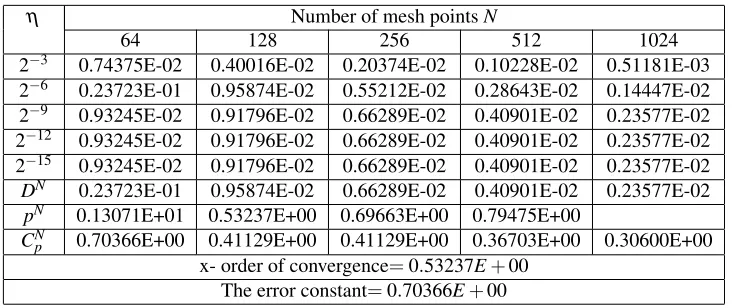
Fixing a fine Shishkin mesh with 32 points horizontally, the problem is solved by the method suggested above. The order of convergence and the error constant are calculated for

tand the results are presented in Table 1. A fine uniform mesh ontwith 32 points is considered and the order of convergence in the variablexis calculated. The results are presented in Table 2. A graph of the numerical solution is presented in the figure 1.

Table 1.Values ofDN,pN,p∗andCN_p∗for

ε1=η/32,ε2=η/16 and α=0.9

η Number of mesh pointsN

64 128 256 512 1024

2−3 0.411094E-02 0.207861E-02 0.104757E-02 0.526658E-03 0.264056E-03

2−6 0.399695E-02 0.202648E-02 0.102043E-02 0.512040E-03 0.256480E-03

2−9 0.399651E-02 0.202636E-02 0.102040E-02 0.512032E-03 0.256478E-03

2−12 0.399635E-02 0.202632E-02 0.102039E-02 0.512029E-03 0.256477E-03

2−15 0.399630E-02 0.202631E-02 0.102039E-02 0.512028E-03 0.256477E-03

DN 0.411094E-02 0.207861E-02 0.104757E-02 0.526658E-03 0.264056E-03

pN 0.983848E+00 0.988567E+00 0.992114E+00 0.996020E+00

CN

p 0.497616E+00 0.497616E+00 0.495991E+00 0.493157E+00 0.489014E+00

t-order of convergence=0.983848E+00 The error constant=0.497616E+00

Table 2. Values ofDN_,_pN_,_p∗_and_CN

p∗ forε1=η/32,

ε2=η/16 andα=0.9

η Number of mesh pointsN

64 128 256 512 1024

2−3 0.74375E-02 0.40016E-02 0.20374E-02 0.10228E-02 0.51181E-03

2−6 0.23723E-01 0.95874E-02 0.55212E-02 0.28643E-02 0.14447E-02

2−9 0.93245E-02 0.91796E-02 0.66289E-02 0.40901E-02 0.23577E-02

2−12 0.93245E-02 0.91796E-02 0.66289E-02 0.40901E-02 0.23577E-02

2−15 _0.93245E-02 _0.91796E-02 _0.66289E-02 _0.40901E-02 _0.23577E-02

DN 0.23723E-01 0.95874E-02 0.66289E-02 0.40901E-02 0.23577E-02

pN 0.13071E+01 0.53237E+00 0.69663E+00 0.79475E+00

CN

p 0.70366E+00 0.41129E+00 0.41129E+00 0.36703E+00 0.30600E+00

x- order of convergence=0.53237E+00 The error constant=0.70366E+00

Figure 1

0 0.5 1 1.5 2

0 0.1 0.2 0.3 0.4 0.5 0.6 0.7 0.8 0.9 1 0.8

1 1.2 1.4 1.6 1.8 2

(14)

9. Conclusion

Thus in this paper, a linear parabolic system of singularly perturbed equations of reaction diffusion type with delay is considered and the suggested numerical method has been proved to be first order convergent, with respect to space and time, theoretically and numerically.

References

[1] _{A. Martin, S. Raun, Predetor-prey models with delay and}

prey harvesting, J. Math. Bio., 43, 2001, pp. 247-267.

[2] _{O. Arino, M.–L. Hbid, E. Ait Dads, Delay Differential}

Equations and Applications, Springer, The Netherlands, 2006.

[3] _{A. Asachenkov, G. Marchuk, R. Mohler, S. Zuew,}

Dis-ease Dynamics, Birkhauser, Boston, 1994.

[4] _{Charles G. Lange and Robert M. Miura,}_Singular

Per-turbation Analysis of Boundary-Value Problems for Differential-Difference EquationsSIAM J. APPL. MATH. Vol. 42, No. 3, June 1982.

Per-turbation Analysis of Boundary-Value Problems for Differential-Difference Equations II. Rapid Oscillations and ResonancesSIAM J. APPL. MATH. Vol. 45, No. 5, October 1985.

Per-turbation Analysis of Boundary-Value Problems for Differential-Difference Equations III. Turning Point

Prob-lemsSIAM J. APPL. MATH. Vol. 45, No. 5, October

1985.

Per-turbation Analysis of Boundary-Value Problems for Differential-Difference Equations. VI. Small Shifts with Rapid OscillationsSIAM J. APPL. MATH. Vol. 54, No. 1, pp. 273-283, February 1994.

[8] _{J. J. H. Miller, E. O’Riordan, G.I. Shishkin,}_Fitted

Nu-merical Methods for Singular Perturbation Problems, World Scientific Publishing Co., Singapore, New Jersey, London, Hong Kong (1996).

[9] _{V. Franklin, M. Paramasivam, J.J.H. Miller and S.}

Valar-mathi, Second order parameter-uniform convergence for a finite difference method for a singularly perturbed lin-ear parabolic system, International Journal of Numerical Analysis and Modeling Vol. 10, No. 1, pp. 178-202.

[10] _{M.Manikandan, N.Shivaranjani, J. J. H. Miller and S.}

Valarmathi, A parameter uniform first order convergent numerical method for a boundary value problem for a sin-gularly perturbed delay differential equation, Advances in Applied Mathematics, Springer Proceedings in Mathe-matics and Statistics 87, pp. 71-88.

[11] _{Manikandan Mariappan, John J. H. Miller and}

Valar-mathi Sigamani, A parameter-uniform first order con-vergent numerical method for a system of singularly perturbed second order delay differential equations, P.Knobloch(ed.), Boundary and Interior Layers,

Compu-tational and Asymptotic Methods - BAIL 2014, Lecture Notes in Computational Science and Engineering 108, Springer International Publishing Switzerland 2015.

[12] _{Parthiban Saminathan, Valarmathi Sigamani and Franklin}

Victor, Numerical Method for a Singularly Perturbed Boundary Value Problem for a Linear Parabolic Second Order Delay Differential Equation, Differential Equa-tions and Numerical Analysis, Springer Proceedings in Mathematics and Statistics(2016), Volume172.

[13] _{A.R. Ansari, S.A. Bakr, and G.I. Shishkin, A}

parameter-robust finite difference method for singularly perturbed delay parabolic partial differential equations, Journal of Computational and Applied Mathematics 205 (2007) 552 – 566

[14] _{Zhongdi Cen, A hybrid finite difference scheme for a}

class of singularly perturbed delay differential equations, Neural, Parallel and Scientific Computations 16, 303-308 (2008).

[15] _{J. J. H. Miller, E. O’Riordan, G.I. Shishkin, L.P.}

Shishk-ina, Fitted Mesh Methods for Problems with Parabolic Boundary Layers, Mathematical Proceedings of the Royal Irish Academy, 98A(2), 173 - 190 (1998).

[16] _{E.P. Doolan, J.J.H.Miller and W.H.A. Schilders, Uniform}

numerical methods for problems with initial and bound-ary layers, Boole Press, 1980.

[17] _{P.A. Farrell and A.F. Hegarty and J.J.H. Miller and}

E.O’ Riordan and G.I. Shishkin, Robust computational techniques for boundary layers, Chapman and hall/CRC, Boca Raton, Florida,USA, 2000.

? ? ? ? ? ? ? ? ?

ISSN(P):2319−3786 Malaya Journal of Matematik

ISSN(O):2321−5666

Parameter uniform numerical method for a singularly perturbed boundary value problem for a linear system of parabolic second order delay differential equations