University of Southern Queensland
Faculty of Health, Engineering & Sciences
Simulation of Fibre Bragg Grating (FBG) Reflection
Spectrums Using OptiGrating
A dissertation submitted by
Byrenn James Colin Birch
in the fulfilment of the requirements of
ENG4111 and ENG4112 Research Project
towards the degree of
Bachelor of Engineering (Mechanical)
Abstract
Fibre composite materials for use in structural applications are becoming more common. However the sudden failures they are susceptible to creates a need for structural health monitoring to ensure safe use. Mechanical fibre composite structures such as wind turbine blades and airframes are desirable to have in operation as long as possible, therefore any structural health monitoring technology capable of operating when the structure is in service is advantageous. This technology is optical sensors, specifically fibre Bragg grating sensors. Fibre Bragg grating sensors can be embedded in composite materials to measure the strain and temperature at a specific location. These measurements can be compared with historical data to assess the health of the structure.
The data is viewed as the reflection spectrum which visually shows the trends and can be analysed numerically. This research intends to reproduce the reflection spectrum using a combination of finite element analysis (FEA) software and OptiGrating. This has the potential to extend academic knowledge and be a step in the development of methods to calculate the actual strain field to which a sensor is subject.
Three different sample were manufactured with known defects and tested. The zero load reflections were imported to OptiGrating and solved using inbuilt functions. Finite element analysis yielded good correlation to the strain calculated from the Bragg wavelength of each physical test. However, when the FEA strain was applied to a virtual sensor in OptiGrating the data did not correlate with the real tests, nor the FEA data.
examination found that this error could be compensated for, thus OptiGrating analysis was repeated. Following the correction the Bragg wavelength correlation was good but due to limitations with the inverse scattering solver and FEA made replicating the behaviour of sidelobes impossible at this stage.
OptiGrating was contacted about these issues. They have confirmed the error in calculating the strain-optic coefficient and are currently developing a version that corrects the issue.
Disclaimer Page
University of Southern Queensland
Faculty of Health, Engineering and Sciences
ENG4111/ENG4112 Research Project
Limitations of Use
The Council of the University of Southern Queensland, its Faculty of Health, Engineering & Sciences, and the staff of the University of Southern Queensland, do not accept any responsibility for the truth, accuracy or completeness of material contained within or associated with this dissertation.
Certification of Dissertation
I certify that the ideas, designs and experimental work, results, analyses and conclusions set out in this dissertation are entirely my own effort, except where otherwise indicated and acknowledged.
I further certify that the work is original and has not been previously submitted for assessment in any other course or institution, except where specifically stated.
Byrenn Birch
0061004717
__________________________
Signature
__________________________
Acknowledgements
My research project was completed under the supervision of Dr Jayantha Epaarachchi. My thanks go to Jayantha for his guidance, support and patience over the duration of the research.
Table of Contents
Abstract ii
Disclaimer Page iv
Certification of Dissertation v
Acknowledgements vi
List of Figures xi
List of Tables xiv
Nomenclature and Acronyms xvi
Chapter 1 - Introduction 1
1.1 Overview 1
1.2 Introduction 1
1.3 Research Objectives and Design 3
1.4 Conclusions 4
Chapter 2 - Literature Review 5
2.1 Introduction 5
2.2 Glass Fibre Reinforced Plastics 6
2.2.1 Structures and Properties 7
2.2.2 Interlaminar Fracture 18
2.2.3 Structural Health Monitoring 21
2.3 Fibre Bragg Grating Sensors 24
2.3.1 Grating Structures 26
2.3.2 Performance, Physics and Principles 28
2.3.3 Interrogation 33
2.3.4 Structural Health Monitoring 34
2.3.5 Effect on Composite Structures 34
2.4 Simulation and Fabrication 35
2.4.1 Finite Element Analysis Using ABAQUS 6.12 35
2.4.2 OptiGrating 36
2.5 Conclusions 37
Chapter 3 - Research Design and Methodology 38
3.1 Project Planning 38
3.1.1 Timeline 38
3.1.2 Resource Requirements 39
3.1.3 Safety 39
3.2 Sample Design 40
3.3 Physical Models 43
3.3.1 Manufacture of Physical Models 43
3.3.2 Testing of Physical Models 56
3.4 Finite Element Analysis Process Using ABAQUS 6.12 59
3.5 OptiGrating 69
3.5.1 Reconstruction of the Grating from the Reflection Spectrum 69
Chapter 4 – Results 78
4.1 Results of Physical Testing 78
4.1.1 Sample A- No Defect 79
4.1.2 Sample A1- 16mm Hole 81
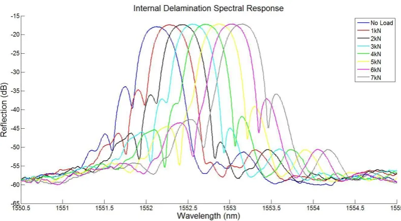
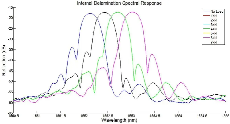
4.1.3 Sample B- Internal Delamination 84
4.1.4 Tabulated Results 86
4.2 Finite Element Analysis Results 87
4.3 OptiGrating Results 95
4.3.1 Original OptiGrating Analysis 96
4.3.2 OptiGrating Analysis using Modified Photo-Elastic Coefficients 105
4.3.3 Visual Analysis of Spectrums 114
Chapter 5 - Discussion 124
5.1 Interpretation of Results 124
5.2 Comparison with the Aim of the Research 130
5.3 Limitations & Improvements 131
5.4 Recommendations 131
5.5 Further Work 132
Chapter 6 - Conclusion 134
Appendices 140
Appendix A- Project Specification 140
Appendix B- Risk Assessment 142
Appendix C- Interrogation Unit Specifications 150
Appendix D- Material Data Sheets 151
Appendix E- Fibre Bragg Grating Sensor Datasheets 153
Appendix F- MATLAB Scripts 155
Appendix F1- Data Manipulation 155
List of Figures
Figure 2.1- Specific Strength, Specific Modulus Chart 7
Figure 2.2- Effect of Fibre Orientation on Tensile Strength 12
Figure 2.3- Lamination Scheme 14
Figure 2.4- Laminate Global Coordinate System 15
Figure 2.5- Idealised Properties of Composite Laminates 16 Figure 2.6- Delamination Sources at Geometric and Material Discontinuities 18
Figure 2.7- Fundamental Modes of Delamination 19
Figure 2.8- Damage Caused by External Impact 20
Figure 2.9- FBG Theory 24
Figure 2.10- FBGS Structure 25
Figure 2.11- FBG Structures 27
Figure 2.12- FBG Spectrum Properties 32
Figure 3.1- Sample Layup 40
Figure 3.2- Sample Design 42
Figure 3.3- Glass Fibre Stack and Markings 45
Figure 3.4- FBGS Placement (Sample B) 47
Figure 3 5- Sensor Arrangement 48
Figure 3.6- Fibre Rolling Process 49
Figure 3.7- Resin Spreading 50
Figure 3.8- Manufacturing Frame 51
Figure 3.9- Sample Design, Actual Dimensions 54
Figure 3.10- Testing Set-up 57
Figure 3.11- Sample Mesh Structure, Sample A1 59
Figure 3.13- Loading Diagram (Sample B) 65
Figure 3.14- Finite Element Analysis Data at 5kN 67
Figure 3.15- Inverse Scattering Solver Output 73
Figure 3.16- Inverse Scattering Solver Output 74
Figure 3.17- FWHM Toolbox Window 77
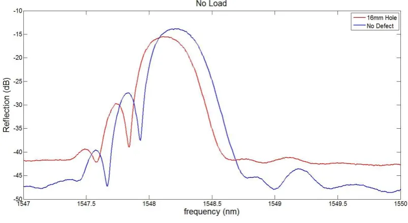
Figure 4.1-Results of Physical Testing, No Defect 79
Figure 4.2- Results of Physical Testing, No Defect 80
Figure 4.3- Results of Physical Testing, 16mm Hole 82
Figure 4.4- Results of Physical Testing, 16mm Hole 82
Figure 4.5- Sample A/A1 Reflection at Zero Load 83
Figure 4.6- Results of Physical Testing, Internal Delamination 84 Figure 4.7- Results of Physical Testing, Internal Delamination 85
Figure 4.8- FEA Sensor Location, Sample A1 89
Figure 4.9- FEA Sensor Location, Sample B 90
Figure 4.10- E11 Strain Field, Sample A1 91
Figure 4.11- E11 Strain Field, Sample B 91
Figure 4.12- Sensor Dialogue Box 97
Figure 4.13- Sensor Dialogue Box, Modified Coefficients 106
Figure 4.14- Comparison of Strain Data, Sample A 112
Figure 4.15- Comparison of Strain Data, Sample A1 113
Figure 4.16- Comparison of Strain Data, Sample B 113
Figure 4.17- Inverse Scattering Solver Result, Sample A 115
Figure 4.18- OptiGrating Results, Sample A 116
Figure 4.21- OptiGrating Results, Sample A1 119 Figure 4.22- Comparison of Real and Simulated Spectra, Sample A1 120 Figure 4.23- Inverse Scattering Solver Result, Sample B 121
Figure 4.24- OptiGrating Results, Sample B 122
Figure 4.25- Comparison of Real and Simulated Spectra, Sample B 123
Figure 5.1- Micro Bending of FBG Sensors 127
List of Tables
Table 2.1- Composition of Glass Fibre Reinforcements 10
Table 2.2- GFRP Manufacturing Methods 13
Table 3.1- Timeline of Research 38
Table 3.2- Properties of FBGS as Specified by Manufacturer 43
Table 3.3- Material Properties of GFRP Lamina 44
Table 3.4- FBG Sensor Data 55
Table 3.5- Tensile Loads Applied to Samples 56
Table 3.6- Representative Micron Optics Text File Format 58
Table 3.7- ABAQUS Material Properties 60
Table 3.8- FEA Composite Layup- Sample A/A1 62
Table 3.9- FEA Composite Layup- Sample B 63
Table 3.10- Applied FEA Loads 66
Table 3.11- Micro-strain Regressions from FEA 68
Table 3.12- FBGS Properties for OptiGrating 70
Table 3.13- Table of Sellmeier Parameters 71
Table 3.14- Micron Optics Text File Format 72
Table 3.15- Strain-Optic Parameters 75
Table 4.1- FBGS Properties 78
Table 4.2- Strain Results of Physical Testing 86
Table 4.3- Regressions of Micro-strain Along FBGS using FEA 92 Table 4.4- Comparison of Finite Element Analysis and Physical Testing 94
Table 4.5- Photo-Elastic Coefficients 96
Table 4.6- Bragg Wavelength Comparison 99
Table 4.8- Strain Comparison, Sample A1 100
Table 4.9- Strain Comparison, Sample B 101
Table 4.10- Calculation of the Strain-Optic Coefficient 103
Table 4.11- Modified Photo-Elastic Coefficients 105
Table 4.12- Bragg Wavelength Comparison (Modified Pij) 108 Table 4.13- Strain Comparison, Sample A (Pij Modified) 109 Table 4.14- Strain Comparison, Sample A1 (Pij Modified) 109 Table 4.15- Strain Comparison, Sample B (Pij Modified) 110
Nomenclature and Acronyms
The following list details the nomenclature and acronyms used in the following text.
3D Three Dimensional
An Amplitude Sellmeier Coefficient
CAD Computer Aided Design
CEEFC Centre of Excellence in Engineered Fibre Composites
CVM Cumulative Vacuum Method
d Fibre Diameter
Ei,j Modulus of Elasticity in i,j Direction
FBG Fibre Bragg Grating
FBGS Fibre Bragg Grating Sensor FEA Finite Element Analysis
FWHM Full Wavelength Half Maximum GFRP Glass Fibre Reinforced Plastic Gi,j Shear Modulus in i,j Direction ISS Inverse Scattering Solver
l Length
L Fibre Bragg Grating Length
lc Critical Length
Lp Sound Pressure Level
N Number of Fibre Fringes
NASA National Aeronautics and Space Administration neff Effective Refractive Index
pe Gage Factor
Pij Photo-elastic Coefficient, ij Direction PPE Personal Protective Equipment
R Reflectivity
S3R Triangular Mesh Element
S4R Quadrangular Mesh Element
Sample A No Defect Test Sample Sample A1 16mm Hole Test Sample
Sample B 24mm Internal Delamination Test Sample SHM Structural Health Monitoring
SI International System of Units
SMF Single Mode Fibre
USQ University of Southern Queensland
UV Ultraviolet
α Coefficient of Thermal Expansion γi,j Shear Strain in i,j Direction
Δ Change in/of
εi,j Strain in i,j Direction κac Coupling Coefficient
𝑘𝑖
⃗⃗⃗ Incident Wavelength
𝑘𝑟
⃗⃗⃗⃗ Reflected Wave
𝐾⃗⃗ Grating Wave Vector
Λ Grating Period
λ1,2,3 Wavelength Sellmeier Coefficient
λB Bragg Wavelength
ν Poisson’s Ratio
νi,j Poisson’s Ratio in i,j Direction
ξ Thermo-optic Coefficient
ρa Photo-elastic Coefficient σi,j Stress in i,j Direction
σf* Ultimate Fibre Tensile Strength τc Fibre-Matrix Bond Strength
τi,j Shear Stress in i,j Direction
Chapter 1 - Introduction
1.1
Overview
The rationale of this research is to investigate the response of 1550nm fibre Bragg grating sensors embedded in glass fibre reinforced plastic samples manufactured with known defects. Three different specimens were subjected to static tensile loading between 0kN and 8kN in 1000 Newton increments. The spectrums found from these tests are to be reconstructed and simulated by use of finite element analysis (FEA) and commercially available integrated and fibre optical grating design software (OptiGrating 4.2). Evaluation of the real and simulated spectrums was completed to gauge the viability and accuracy of using a combination of software to recreate real grating reflection spectrums for the purposes of further research and development of structural health monitoring (SHM) technology.
1.2
Introduction
cumulative vacuum method (CVM), ultrasound and Bragg grating sensors. When considering SHM of mechanical structures such as turbine blades and airframes, the structure must be taken out of service for CVM and ultrasound. Alternatively optical fibre Bragg grating (FBG) sensors can be used to provide live feedback of a structure in service.
In addition to embedded FBG sensors being able to provide live feedback, they have the following advantages over other SHM methods:
Do not require calibration
No length limits due to very small losses in optical fibres
Passive technology (no electrical components)
Immune to electromagnetic fields
Long term stability
FBG sensors can be embedded into the composite material without compromising the mechanical performance of the material. For SHM applications, FBG sensors can be used to measure mechanical strain and temperature. In this research testing was done in isothermal conditions to circumvent the temperature sensitivity of the sensor and focus entirely on mechanical strain.
Finite element analysis was completed using the composite layup analysis tools in ABAQUS 6.12. The strain field along the sensor was calculated and applied to the virtual sensor created in OptiGrating from known data.
The resultant simulated spectrums were then compared to the real spectrums to assess the viability of using OptiGrating for simulating real reflection spectrums.
1.3
Research Objectives and Design
The objectives of this research are:
1) To analyse the use of FEA for defect analysis and simulation of composite structures, including delamination
2) To reproduce and simulate a real FBG reflection spectrum using OptiGrating
These objectives are summarised into the following statement of aim:
‘To analyse the efficacy of using a combination of finite element analysis and OptiGrating software to replicate and simulate real Bragg reflections’
To achieve the aim, the research was divided into the following phases:
Background Research
o Glass fibre composite materials and manufacture o FBG sensors
o FEA
o OptiGrating
Simulation
o FEA and OptiGrating
Analysis of results
Background Research is contained in Chapter 2 - Literature Review and the findings of this was used to design the experimentation phases.
Physical experimentation involved the design, manufacture and testing of composite samples. These samples were reproduced in ABAQUS 11.2 and relevant loads simulated. The results of FEA were applied to the virtual sensor in OptiGrating. The results of physical experimentation were compared to the results of simulation. Analysis of these results included visual analysis of sidelobe trends and calculation of mean mechanical strain from the Bragg wavelength. Critical investigation and discussion was provided to analyse the source of any errors or deficiencies in either the project design or the programs used.
1.4
Conclusions
Chapter 2 - Literature Review
2.1 Introduction
This chapter analyses literature to establish the need for continual structural health monitoring (SHM) of advanced fibre composites, specifically delamination defects. Published academic works will be reviewed; detailing the need for SHM of fibre composites, current methods for detecting and monitoring delamination defects, and the use of fibre Bragg grating sensors in composite structures. Additional research detailing the use of finite element analysis (FEA) software to model damage to composite structures, and the use and efficacy of OptiGrating to simulate and generate FBG spectra will be conducted. The review will also explore fabrication methodologies and testing procedures for fibre composites.
The reviewed literature will enhance the research, continually reflecting and relating to the project objectives.
2.2 Glass Fibre Reinforced Plastics
Glass fibre reinforced plastics (GFRPs) are composite materials comprised of a polymer matrix reinforced with glass fibres. The most common type is known as fibreglass or E-glass. GFRPs are now a reasonable substitute for traditional structural materials, such as steel, due to the improvement of their mechanical properties over time (Deshmukh & Jaju 2011). They are most commonly used in applications requiring a high strength to weight ratio, customisable mechanical properties and applications requiring chemical and corrosion resistance (Reddy & Miravete 1995). The reduction of weight offered by composite structures has been described by Karbhari, Steenkamer and Wilkins (1997) as three main benefits in civil structures. They are;
1. Lower dead weight enabling a higher live load capacity for the same supporting structure (in the case of replacement structures)
2. Lower dead weight enabling the use of lighter and smaller supporting structures in new structures
3. Lower dead weight enabling greater ease of field placement without heavy equipment
2.2.1 Structures and Properties
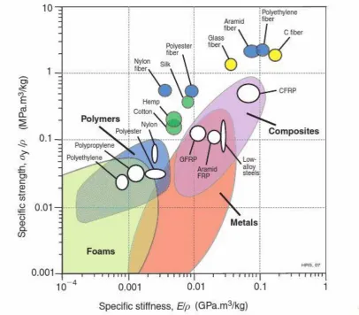
[image:26.595.115.522.245.601.2]Glass fibre reinforced plastics are composite materials comprised of a polymer matrix reinforced with glass fibres. Figure 2.1 (Ashby 2007) compares the specific strength and specific modulus of different materials. The figure shows that GFRPs have similar specific strength and specific modulus values to high performance metals, thus in many situations can be viable alternatives to traditional materials.
Figure 2.1- Specific Strength, Specific Modulus Chart (Ashby 2007)
dominant contributors to the mechanical properties of the composite. Callister (2007) and Deshmukh and Jaju (2011) agree that the dominant contributors to the mechanical properties of a material are;
The properties of the matrix
The properties of the fibre
Fibre size and shape
Fibre concentration
Fibre orientation
Matrix Properties
Askeland and Phule (2008) state that the purpose of the matrix is to;
support the fibres
fix their orientation
transfer load to the fibres
protect the fibres from damage
Matrices are either thermoset or thermoplastic materials. Juska and Puckett (1997) state that thermoplastic composites typically have poor compressive strength, and are expensive and difficult to manufacture. Currently they have little application in primary structural composites (ENG8803 Mechanics and Technology of Fibre Composites 2008). Conversely thermoset polymers are widely used. Thermoset resins are generally low viscosity and can be formed at room temperature. Thermosets are stiffer and stronger than thermoplastics, however typically have lower elongations and toughness. Due to the limited use for thermoplastics in composite materials, thermoset resins and materials will be considered in this report.
Fibre Properties
Table 2.1- Composition of Glass Fibre Reinforcements
TYPE A C D E ECR AR R S2
% % % % % % % %
SIO2 63-72 64-68 72-75 52-56 54-62 55-75 55-65 64-66
AL2O3 0-3 4-5 0 15 14 - 15-30 24-25
B2O3 0-1 4-5 21-24 10 - 0 - -
CAO 9 13-14 0 16-25 17-25 0-10 2-10 0-0.1
MGO 1 3-4 - - - - 5-20 9.5-10
ZNO - - - - 1 - - -
BAO - - - - - - - -
LIO - - - - - 0-1.5 - -
NA2+K2O 14-16 9-10 - - - - - 0-0.2
TIO2 0-0.6 - - 0-1.5 - - 0-0.3 -
ZRO2 - - - - - 16-20 - -
FE2O3 0-0.5 0-0.8 0-0.3 0-0.8 0-0.8 0 - 0-0.1
F 0-0.4 - - 0 - - 0-0.3 -
*E-Glass is bolded as it is used in the experiment
Fibre Size and Shape
As already stated, the function of fibres in fibre reinforced composite materials is to transfer strength to the matrix constituent and enhance its properties. However, the ability of the fibre to accomplish this is related to the fibre length. Askeland and Phule (2008) state that ‘… there is no load transmittance from the matrix at each fibre extremity’. Consequently, there is a critical length of fibre necessary for effective strengthening and stiffening of the composite. The critical length (lc) is defined as;
lc =
𝜎𝑓∗ ∙ 𝑑
2 ∙ 𝜏𝑐 (2.1)
where;
𝜏𝑐 is the fibre-matrix bond strength
Typical glass fibre diameters range between 3 and 20 μm. When the fibre length is equal to lcthe maximum fibre stress occurs only at the axial centre of the fibre. As the
length of the fibre increases, the reinforcement becomes more effective. If the length of the fibre is greater than 15lc the fibre is classified as continuous (Callister 2007).
Continuous fibres are the most effective in improving the composite materials’
strength. Lengths below this, but greater than the critical length are discontinuous fibres, while if the length is less than lc the fibre is short. Short fibres are least effective
as the matrix tends to carry the load. The matrix deforms around the short fibres and transfers very little stress (Pan 1993). Campbell (2010) also states that in general; the smaller the fibre diameter, the greater the higher the strength. This however increases cost. Therefore it is clear that the fibre size effects the performance of composite materials.
Fibre Concentration
Fibre Orientation
The orientation of fibres has a large impact on the material properties of a composite. Continuous unidirectional fibres form anisotropic properties (Askeland & Phule 2008). These materials are strong parallel to the fibre direction, and weak in other directions. Figure 2.2 illustrates the effect of fibre orientation on the tensile strength of E-glass fibre reinforced epoxy composites (Askeland & Phule 2008; Callister 2007). To compensate for this behaviour, fibre composites are arranged into laminates. This practice allows a laminate to have desired properties in multiple directions.
Manufacture
There are six common methods for manufacture of continuous polymer matrix composites as listed in Table 2.2 (Campbell 2010). The resources available at the Centre of Excellence in Engineered Fibre Composites (CEEFC) and the suitability of the manufacturing method for embedding FBG sensors in a small number of samples meant only hand layup was a viable option.
Table 2.2- GFRP Manufacturing Methods
METHOD THERMOSET THERMOPLASTIC
HAND LAYUP
FILAMENT WINDING
PULTRUSION
LIQUID MOULDING
THERMOFORMING
COMPRESSION MOULDING
Laminas and Laminates
A disadvantage of the laminate structure is the introduction of shear stresses being introduced between the laminas (Reddy 2004). This phenomena is a major cause of interlaminar fracture. For clarity in further sections, the global coordinate system for composites is shown in Figure 2.4. The 1-axis is parallel to the fibre direction, 2 is the in-plane perpendicular, and the 3-axis is the out-of-plane perpendicular.
Mechanics of Laminates
When analysing laminate materials, it is convenient to idealise the mechanical properties of the laminate (Figure 2.5).
Figure 2.5- Idealised Properties of Composite Laminates (ENG8803 Mechanics and Technology of Fibre Composites 2008)
The relationship between stress and strain in transversely isotropic materials is; [ ε11 ε22 ε33 γ23 γ31 γ12]
= [ 1 E11 -ν21 E22 -ν21
E22 0 0 0
-ν12 E11
1 E22
-ν23
E22 0 0 0
-ν12 E11
-ν23 E22
1
E22 0 0 0
0 0 0 2(1+ν23)
E22 0 0
0 0 0 0 1
G12 0
0 0 0 0 0 1
G12] ∙ [ σ11 σ22 σ33 τ23 τ31 τ12]
(2.2)
where;
ε represents strain
γ represents shear strain
E represents the Modulus of Elasticity
G represents the Shear Modulus
ν represents Poisson’s ratio
σ represents the stress
τ represents shear stress
2.2.2 Interlaminar Fracture
Interlaminar fracture, or delamination is the separation of the fibre-reinforced lamina with a laminate (O'Brien 2001). Due to the nature of the dissertation, this section considers the overall phenomena of interlaminar fracture, but not the specific mechanics of delamination. Delamination can be caused my mismatches in material properties, either between layers or matrix and fibre, or introduced via manufacturing flaws (Reddy 2004). The interlaminar fractures initiated by mismatches in material properties between lamina causes shear stresses to occur between layers (Reddy & Miravete 1995). Similarly, the mismatch of material properties between the fibres and matrix can result in fibre debonding. These delaminations typically occur at stress-free edges (O'Brien 2001), both internal and external. Reddy (2004) states that manufacturing defects are impossible to eliminate. These manufacturing defects are caused by material defects, including interlaminar voids, incorrect fibre orientation, damaged fibres and delaminations. Figure 2.6 illustrates common sources of delaminations at geometric discontinuities (O'Brien 2001).
O'Brien (2001) also states there are three fundamental modes of final delamination failure;
Mode I: Opening mode
Mode II: In-plane scissoring mode
Mode III: Tearing or scissoring shearing mode
These modes are best explained by Figure 2.7. In reality, delaminations occur due to a combination of these modes, as loads are seldom ideal. These are called mixed mode failures.
Figure 2.7- Fundamental Modes of Delamination (O'Brien 2001)
2.2.3 Structural Health Monitoring
Structural health monitoring (SHM) is the process of implementing damage detection and characterisation strategy for engineering structures. The field is borne from the need to build and maintain safe structures. The continual monitoring of a structures health is imperative to critical components as ‘…one can never know enough in terms of the material’s properties as well as the environment the structure is going to operate in’ (Encyclopedia of Structural Health Monitoring 2009). SHM has the potential to decrease inspection costs of composite components, currently one-third of the total manufacturing and operation cost of the component (Soutis & Diamanti 2010). The prevalence of composite structures in modern engineering, especially aviation, makes SHM of critical importance, due to the sudden failures composites are susceptible to. As of 2009, Airbus was considering the following SHM methods (among others) for their composite components;
comparative vacuum method (CVM)
optical fibre sensors (FBG)
acoustic emission
CVM is a surface mounted monitoring technique. It utilises an adhesive backed patch containing small tubes. Once applied to the surface by hand pressure, any pressure changes leak to the vacuum and detection can be completed. This method is passive, and can only be used periodically.
Acoustic emission can detect differences in structures of composite sheet materials. This method is also a periodic inspection.
These methods for SHM can be used as an alternative to, or in conjunction with more common non-destructive inspection techniques (Soutis & Diamanti 2010) such as;
Visual inspection
Ultrasonic inspection
Radiographic inspection
These methods are all periodic inspections of the structure.
2.2.4 Simulation of Interlaminar Fracture Defects
2.3 Fibre Bragg Grating Sensors
A fibre Bragg grating (FBG) is defined as ‘a periodic or aperiodic perturbation of the
effective refractive index in the core of an optical fibre’ (Paschotta 2013). These perturbations are formed in the core of the fibre by the means of exposure to intense short wavelength (<300nm) ultraviolet (UV) radiation along the length of the grating, disrupted by an interference pattern (Hill & Meltz 1997). Short wavelength UV radiation produces enough energy to break the highly stable silicon-oxygen bonds within the core material (Doyle 2003). This damages the structure of the fibre and causes a slight increase to its refractive index. These inscriptions in the fibre core form the grating. The distance between these inscriptions is called the index variation. When light travels down the core, the wavelengths corresponding to the index variation are reflected. This is best illustrated by Figure 2.9.
Fibre Bragg grating sensors (FBGS) contain three regions; inner core, cladding and a protective coating (Figure 2.10). The inner core can range from 4-9μm and has a higher refractive index than the cladding due to high germanium doping. This difference in refractive index causes light to propagate in the core only (Ashby 2007). The best suited core and cladding material is pure glass (SiO2), or fused silica. The cladding has a diameter of 125μm. The protective coating is comprised of either acrylate, polyimide or ORMOCER (organic modulated ceramic). This layer protects the sensor from hydrogen and water. These contaminants cause crack growth and can decrease mechanical stability from greater than 30 000 strains to less than 5 000 micro-strains. It is important to note that FBGS measure strain, not displacement.
Figure 2.10- FBGS Structure
immune to electromagnetic interference and are intrinsically passive since they require no electrical power. They also have minimal magnetic field interactions and good corrosion resistance (Ferdinand et al. 2002). However, FBGS also have their disadvantages. They exhibit high temperature dependence, where a 1oC change corresponds to approximately eight micro-strains (Kreuzer 2006). FBGS have a high stiffness. This causes increased parallel forces in the specimen. FBGS are also highly sensitive to lateral forces or pressure. This sensitivity causes light birefringence. Birefringence causes multiple peaks to occur in FBG spectra. However, Wang et al. (2006) states that; ‘… the length of a FBG is much longer than the diameter of the fibre and it is reasonable to assume loading situations to be contained in a single plane.’ Consequently, should a FBG sensor be measuring principle axial strain, the spectra represents the in-plane strains occurring at the fibre. For example, if measuring ε11 with a FBG, ε22 will have an effect, but not ε33.
2.3.1 Grating Structures
There are many grating structures available for different applications. They are achieved by varying the induced index change along the fibre axis. The six most common grating structures are shown in Figure 2.11. Erdogan (1997) describes these structures as:
a) Uniform with positive only index change b) Gaussian apodised
e) Discrete phase shift f) Superstructure
Figure 2.11- FBG Structures (Erdogan 1997)
further information on the damage location. Discrete phase shift gratings and superstructures are also used in telecommunications as dispersion filters.
All structures can be used in the sensor application, however as uniform gratings are most commonly used, they will be used in this research.
2.3.2 Performance, Physics and Principles
When analysing spectral data for FBGS, the reflected spectrum is of most interest. The point of maximum reflectivity is known as the Bragg wavelength, and is denoted by
B. The Bragg wavelength depends on the effective refractive index of the core (neff)
and the grating period (). Chen and Lu (2008) state the relationship between these
parameters can be derived from the principle of the conservation of energy and momentum as demonstrated in equations 2.3 to 2.5, with the final form shown in Equation 2.6.
To satisfy the conservation of energy, reflections from the grating planes cannot alter the frequency (λ). To satisfy the conservation of momentum, the sum of the incident
wavelength 𝑘⃗⃗⃗ 𝑖and the grating wave vector 𝐾⃗⃗ must be equal to the wave vector of the reflected wave 𝑘⃗⃗⃗⃗ 𝑟.
ki
⃗⃗⃗ + K⃗⃗ = k⃗⃗⃗ r (2.3)
To satisfy the Bragg condition, 𝐾⃗⃗ has a direction normal to the grating plane with a magnitude of 2𝜋
ki
⃗⃗⃗ = – k⃗⃗⃗ r (2.4) Consequently, Equation 2.3 can be expressed as;
2𝜋 𝜆𝐵
∙ 𝑛𝑒𝑓𝑓 +
2𝜋
𝛬 = – 2𝜋 𝜆𝐵
∙ 𝑛𝑒𝑓𝑓 (2.5)
which then simplifies to
λB = 2 ∙ neff ∙ Λ (2.6)
Equation 2.6 clearly shows that the Bragg wavelength is affected by any variation in the physical or mechanical properties of the grating region (Doyle 2003). These changes can be attributed to the stress-optic and thermo-optic effects. The stress-optic
effect varies both neff and while the thermo-optic effect changes only neff. Consequently, the change in Bragg wavelength (ΔλB) can be expressed as shown in
equation 2.7.
∆λB = λB ∙ (1 - ρα) ∙ ∆ε + λB ∙ (α + ξ) ∙ ∆T (2.7) where;
ρα represents the photo-elastic coefficient
∆ε represents the change in strain
α represents the coefficient of thermal expansion
ξ represents the thermo-optic coefficient
The photo-elastic coefficient is defined by Optiwave (2008) as;
𝜌𝛼 =
1 2 ∙ 𝑛
2 ∙ [𝑃
12 − 𝜈 ∙ (𝑃11 + 𝑃12)] (2.8)
where;
n represents the core refractive index
It is important to note that the core refractive index, n, is not constant, but varies along the grating length. For uniform gratings, the refractive index profile is;
n(x) = n0 + ∆𝑛 ∙ cos (2𝜋
𝛬 ) (2.9)
where; Δn is the amplitude and induced refractive index perturbation, and x is the distance along the grating (Chen & Lu 2008).
Analysing Figure 2.9 and Figure 2.12, the spectral response has an amplitude. This is known as reflected power in the reflected spectrum and is dependent on reflectivity on the grating. Arora et al. (2011) state that reflectivity is dependent upon grating length and grating period. Arora et al. (2011) demonstrates how the reflectivity of a uniform grating varies upon its length (l), and states the reflectivity of such gratings at the Bragg wavelength is;
Figure 2.12- FBG Spectrum Properties
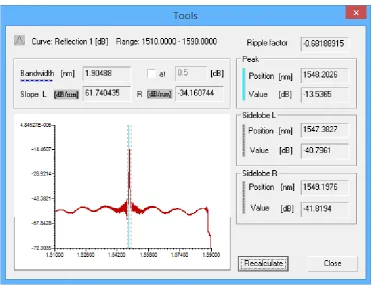
Figure 2.12 identifies the bandwidth and FWHM (full width half maximum). The bandwidth is the distance between the zeros either side of the Bragg wavelength and is easily measured. Kreuzer (2006) defines FWHM as the width across a profile when the value is at half its peak, and is the output given by OptiGrating. FWHM can be simply defined by;
FWHM = 2 ∙ 1.8955 ∙ 𝜆𝐵
𝜋 ∙ 𝑁 (2.11)
where N represents the number of fringes in the fibre and can be given by;
N = 2 ∙ 𝜋 ∙ 𝐿
𝜆𝐵 (2.12)
Comparatively, Kashyap (1999) defines the bandwidth as;
Bandwidth = 𝜆
2
𝜋 ∙ 𝑛𝑒𝑓𝑓 ∙ 𝐿 ∙ √(𝜅𝑎𝑐 ∙ 𝐿)2 + 𝜋2 (2.13) Where κ is a coupling coefficient.
Figure 2.12 also identifies side lobes. Side lobes appear because of multiple partial reflections to and from the opposite ends of the grating region (Chen & Lu 2008). They can be suppressed by the process of apodization. Apodization is the process of varying the strength of the index modulation along the length of the grating (Paschotta 2013).
2.3.3 Interrogation
2.3.4 Structural Health Monitoring
As mentioned in section 2.2.3 Structural Health Monitoring, the main benefit of FBG sensors is they can be embedded in a structure and give live feedback without having to take the component out of service (mechanical application). FBGS are immune to electromagnetic fields (Kahandawa et al. 2012) and intrinsically passive as they use light, not electricity. Embedded FBG sensors are capable of monitoring internal damage which cannot be done with traditional surface mounted strain gages.
2.3.5 Effect on Composite Structures
Barton et al. (2001) analysed the mechanical interactions between an optical fibre and the host material. It was concluded that for a passive optical fibre embedded in the 00 ply of a cross-ply glass fibre laminate, initiation of matrix cracks are insusceptible to the presence of the optical fibre when subject to quasi static loading. However, Barton et al. (2001) explains that under fatigue loading the interaction can cause crack growth, but not development. One challenge of note is the position of the optical fibre, which may move significantly in relation to the 0/90 ply interface (Barton et al. 2001).
2.4 Simulation and Fabrication
This section provides an introduction to the simulation of physical testing- detailing major software used in the project; ABAQUS 6.12 and OptiGrating 4.2. Chapter 2.4 aims to provide the foundation for Chapter 3- Research Design and Methodology, and more detailed analysis of the procedures is provided there.
2.4.1 Finite Element Analysis Using ABAQUS 6.12
ABAQUS/CAE (Complete ABAQUS Environment) 6.12 is a program included in the SIMULIA system published by Dassault Systèmes that uses the finite element method to model and analyse components of a structure (Dassault Systèmes 2013).
ABAQUS allows the importation of geometry from many CAD (Computer Aided Design) packages, but also has a built in part creation module. Complex models can be created and analysed in the software through the use of interactions, sections, different materials and connections. ABAQUS was selected for use over other available software packages because of its ability to analyse composite structures through use of the built in composite layup module. The module allows for definition of composite layups with different materials. This allows the user to view the behaviour at different points in each ply.
has the capability of displaying the strain field in any direction by defining various coordinate systems. It also has a built in composite layup viewer that allows visualisation of composite mechanics, such as strain parallel and perpendicular to the fibre direction and interlaminar strains. The process used in this research is defined further in section 3.4 Finite Element Analysis Process Using ABAQUS 6.12.
2.4.2 OptiGrating
OptiGrating is software by Optiwave used for integrated and fibre optical design (Optiwave 2008). Version 4.2 is used in this project. The software allows adjustments to the fundamental properties (shape, length, apodization, index modulation) of a Bragg grating to me modified for analysis. Strain fields along the sensor can be programmed, and the reflected spectrum calculated by coupled mode equations via the transfer matrix method for solving matrices.
2.5 Conclusions
Chapter 3 - Research Design and Methodology
3.1 Project Planning
3.1.1 Timeline
Table 3.1 shows the time planning required for the research. The ranges shown are for 2013. As shown in this table the planned timeline was not strictly adhered to as different issues arose.
Table 3.1- Timeline of Research
Task Planned Date Range Actual Date Range
Topic Allocation Jan – Mar Jan – Mar
Literature Review Jan – Jun Jan – Sep
Design and Manufacture June July
Physical Testing June July
FEA July July
OptiGrating Analysis Aug Aug – Sep
Project Seminar Sep Sep
Dissertation Jan – Oct Jan – Oct
3.1.2 Resource Requirements
The resources required for the research project were all available at USQ (University of Southern Queensland) and the CEEFC. Consultation with relevant staff and the supervisor found the materials for manufacture and test equipment were available for use with relevant supervision. Access to ABAQUS 11.2 was available at the P2 laboratory, while OptiGrating was loaned for use on a personal computer. All other software was installed on a personal computer.
3.1.3 Safety
The safety aspects of the project were again split into two categories; physical testing and simulation. Simulation only required use of computers and measurement of the physical specimens and was of insignificant consequence with a very rare probability of injury. The physical manufacture and testing was of higher risk and personal protective equipment (PPE) and assistance by trained CEEFC staff. There were no manual handling concerns. A risk assessment is included in Appendix B- Risk Assessment. The following PPE were used at various stages:
Enclosed footwear
Gloves
Overalls
P2 respiration mask
3.2 Sample Design
The laminate samples to be manufactured and tested are to comprise of ten uniaxial lamina in the [0/90/45/-45/0]s configuration as shown in Figure 3.1. This configuration allows a generic composite to be analysed. Samples are to be 300 mm by 100 mm, with defects occurring in the geometric centre of the fibre sheet.
Figure 3.1- Sample Layup
The three samples for manufacture are nominally 100mm by 300mm with ten lamina per laminate;
Sample A
o No defect
o Sensor placed 25mm from long edge
Sample A1
o 16mm hole drilled in Sample A post curing and analysis of Sample A
Sample B
o 24 mm square delamination located between layers 8 and 9 o Sensor placed 5mm from edge of defect
Figure 3.2- Sample Design
Sensors are to be placed between layers 9 and 10, running parallel to the long edge of the sample. The centre of the sensor is located 150 mm from the short edge of the samples. These dimensions are to be checked post curing and cutting to produce accurate finite element analysis models.
Uniform fibre Bragg grating sensors for embedding in samples were sourced from Technica SA and manufactured by the phase mask method.
Table 3.2- Properties of FBGS as Specified by Manufacturer
Sample B Samples C, C1, C2
Centre Wavelength (nm) 1552 ± 0.3 1548 ± 0.3
FBG Length (mm) 5 5
FWHM Bandwidth (nm) < 0.5 < 0.5
Fibre Type SMF-28C SMF-28C
Reflectivity (nominal) >50 % >50 %
Reflectivity (tested) 54.291% 55.125%
3.3 Physical Models
3.3.1 Manufacture of Physical Models
Table 3.3- Material Properties of GFRP Lamina
Material Property Unidirectional E-Glass Unit
E1 34 412 MPa
E2 6 531 MPa
ν12 0.217 -
G12 2 433 MPa
G13 2 433 MPa
G23 1 698 MPa
As three samples of equal size and layup are to be manufactured, they were to be made as one large laminate and cut. This results in a plate of size 300x300 mm. However allowing for wastage the plate was designed larger than this size and sample locations marked on layers eight to ten. These markings allow for accurate alignment of the fibre sheets with critical points (defect/sensor).
To manufacture using this method, ten sheets of E-glass were cut of size greater than 300x300mm. The layup required;
Four sheets of 00 fibre orientation
Two sheets of 900 fibre orientation
Two sheets of 450 fibre orientation
Two sheets of -450 fibre orientation
To make this process more efficient, six were cut for 00 orientation and four at 450 orientation. Sheets were cut using scissors.
for 10% wastage, 605 grams was prepared. The resin to hardener ratio is manufacturer specified as 4:1, therefore 484 grams of resin was mixed with 121 grams of hardener until a consistent colour was achieved, indicating uniform mix.
The specimen was to be manufactured on a glass plate. The glass plate required thorough cleaning with a scraper and acetone to remove any contaminants. For ease of removal of the cured specimen, a minimum of six wax layers were applied to the glass upon recommendation of the CEEFC (Centre of Excellence in Engineered Fibre Composites).
The layers of the glass were then stacked on the glass in correct layup orientation, with sample and defect locations marked as shown in Figure 3.3. Note that markings extend onto lower layers for alignment.
The top layer was removed from the stack for further work, while the remainder of the glass fibre stack was then inverted and placed near to the glass plate. By inverting and taking care in orientating the inverted stack, layers could then be flipped onto the plate in the correct orientation.
To prepare the top layer for the sensors, small openings were made in the fibre sheet with the tip of a ballpoint pen. These were located in line with the desired sensor location and can be viewed in the centre of Figure 3.3 as two red dots spaced approximately 100mm apart.
Sensors were then prepared. To protect the grating region, the sensor was fed through a protective zero tube jacket. One jacket was to go past the grating region while the other was to encapsulate it. Following this the distance along the FBGS from connector to the point where it was to enter the composite was measured. A length of orange tubing was cut to this measurement, and the sensor inserted into this tubing.
The sensor arrangement is shown in Figure 3 5. This image represents the top side of layer ten. Following this process extra care must be taken with this layer as the grating regions are fragile.
Figure 3 5- Sensor Arrangement
Approximately ten percent of the resin/hardener mix was poured onto the lubricated glass. The resin was then evenly spread over the glass to cover sufficient are to place layer one onto. Once layer one was placed in the correct orientation, a fibreglass roller was used to force the resin into the matting. At this step it is important to roll parallel to the fibres so not to damage them and introduce defects (see Figure 3.6).
Insertion Points
Zero Tube Orange Protective
Figure 3.6- Fibre Rolling Process
Figure 3.7- Resin Spreading
Upon completion of layer eight, the interlaminar fracture was introduced by placing a 20mm square of parchment paper in the desired location. The parchment paper was coloured blue for visibility. Using parchment paper as a delamination analogue is common at the CEEFC. It was preferred over Teflon tape due to its superior workability after dry experimentation. Parchment paper was less prone to buckling and unwanted deformation when compared to Teflon tape. This was key when considering the finite element analysis model. Additionally parchment paper could be cut into any shape with ease, while Teflon tape was only readily available in 12mm wide rolls.
To avoid contact between resin and the free sensor and protective layers a frame was placed over the work area. The final layer was then positioned carefully. Both sensors were pulled tight to align the sensors to their desired location. The frame arrangement is shown in Figure 3.8.
Figure 3.8- Manufacturing Frame
and another lubricated glass plate applied onto the sample. This would provide a smooth finished surface. However this is not possible with the sensors protruding from the samples. Consequently the final finish was rough.
After sufficient fibre wetting, silicone was applied to the surface insertion points for strain relief. The sample was then left to cure. Once cured the sample was removed from the glass plate using a scraper.
The samples were cut using a wet saw to produce a smooth cut. Parts of the sensor protruding from the composite were fixed in place with tape during the cutting process.
Once the three samples were cut, any sharp edges were lightly sanded for safety reasons. This process was not anticipated to introduce any defects or stress concentrations. The samples were placed on a light box for visual quality examination. The inspection discovered small bubbles in the samples. The bubbles were sparse and importantly a distance from the sensors. It was decided they would not significantly impact on the fibre Bragg grating sensor, nor the material properties.
engineering judgement made as to consider pure axial strain, maximum resultant strain or a value between.
The length of the sample was designed to be sufficient to overcome strain concentrations at loading points and use Von Mises strain theory. As a result the location of holes to be drilled post curing could be relocated to the desired location without adversely affecting the validity of the analysis. However drilling was inaccurate and resulted in the hole being misaligned with the sensor. This must be considered when conducting the finite element analysis.
The measured dimensions of each sample are as follows. These dimensions are used to create the FEA model.
Sample A
o No defect
o Sensor located 23mm from long edge o 99mm x 300mm
Sample A1
o 16mm hole drilled in centre of Sample A post curing and analysis of Sample A
o Hole and centre centres 4mm misaligned
Sample B
o 96mm x 300mm
o 24mm square delamination located between layers 8 and 9 o Sensor located 4mm from edge of defect, centres aligned
Figure 3.9- Sample Design, Actual Dimensions
The datasheets for the sensors are appended in Appendix E- Fibre Bragg Grating Sensor Datasheets, page 153. Table 3.4 shows the data affixed to the box containing the sensor.
Table 3.4- FBG Sensor Data
Sample A, A1 Sample B
Centre Wavelength (nm) 1548 ± 0.3 1552 ± 0.3
FBG Length (mm) 5 5
Reflectivity >50% >50%
Fibre Type SMF-28C SMF-28C
3.3.2 Testing of Physical Models
The following tensile tests were conducted at the P9 testing facilities located at the CEEFC.
Table 3.5- Tensile Loads Applied to Samples
Sample A (No Defect) Sample A1 (Hole) Sample B (Internal Delamination)
1 kN
2 kN
3 kN
4 kN
5 kN
6 kN
7 kN
8 kN
The equipment used in the testing was;
100kN MTS electromechanical tensile testing machine
Micron Optics interrogation unit
Laptop for viewing and saving data
file for further analysis. The testing set-up is shown in Figure 3.10 showing Sample A1 being tested.
Figure 3.10- Testing Set-up
Data was collected in the 1510 to 1590nm range (1.51x10⁻³ to 1.51x10⁻³ mm) with a delta wavelength of 5pm (5x10⁻⁹mm). This resulted in 16001 data points. The reflected spectrum output was in decibels.
Only channel one of the interrogation unit was connected, consequently the outputs for channels two, three and four were zero. Therefore, Table 3.6 shows the format of the saved text files. The first three and final two rows of data for Sample A1 loaded at 8kN is shown. Note that only the data appears in the text files, not descriptions.
Interrogation Unit
100kN Tensile Test
Laptop
Tensile Test Control
Table 3.6- Representative Micron Optics Text File Format
Column 1 Column 2 Columns 3-5
Wavelength (nm) Channel 1 Reflection (dB) Channels 2-4 Reflection (dB)
1510.000 -44.820 0.000
1510.005 -44.870 0.000
1510.010 -44.790 0.000
⋮ ⋮ ⋮
1589.995 -46.200 0.000
1590.000 -46.230 0.000
3.4 Finite Element Analysis Process Using ABAQUS 6.12
The physical models were modelled in ABAQUS CAE v6.12. The finite element analysis parts were defined as three dimensional (3D) deformable planar shells. ABAQUS is a dimensionless program, and does not allow units to be defined. For clarity and simple consistency, SI (Système Internationale, or International System of Units) was used throughout the analysis.
The geometry of each sample was created as a shell planar feature. For controlled structured meshing in the vicinity of the sensor, the face of the sketch was partitioned for each sample. The edges of the partitioned mesh were seeded at an approximate size of 0.001 (1mm), while the sample edges were seeded with 0.002 (2mm) sizing. This resulted in a fine to very fine mesh with a structured section at the sensor for simple data extraction. Figure 3.11 shows a section of mesh from the FEA model of Sample A1. This mesh structure is representative of the meshes used for each sample. The elements used in the mesh are S3R and S4R.
In addition to partitioning the face of the part for mesh control, the internal delamination region was partitioned. This partition was of the same size as the defect in the same location.
After mesh definition, the parts were assigned materials. The composite used in this research had previously been repeatedly tested by the CEEFC and their researchers. Consequently the mechanical properties of the lamina were obtained from the CEEFC and is shown in Figure 3.6. To analyse the internal delamination, the partitioned region was assigned a different material to that of the samples. This new material was is identified as the pseudo layer/material. It is required for creating the composite layup. The properties of the pseudo layer are shown in Figure 3.6.
Table 3.7- ABAQUS Material Properties
Material Property E-Glass Pseudo Layer Description
E1 34 412 000 000 1
Longitudinal Young’s Modulus
(Pa)
E2 6 531 000 000 1
Transversal Young’s Modulus
(Pa)
Nu12 0.217 0.217 Poisson’s Ratio
G12 2 433 000 000 1
Longitudinal Shear Modulus (Pa)
G13 2 433 000 000 1
Longitudinal Shear Modulus (Pa)
The pseudo layer was required to simulate a perfect delamination. The physical models used parchment paper as a delamination analogue, but it was decided the FEA would be completed with the use of the pseudo material. There is no contact for a perfect delamination, thus the pseudo material must simulate a region devoid of material. To obtain the material properties of the pseudo material, engineering judgement was used in conjunction with the definition of each material property.
Modulus of elasticity is defined as the gradient of the linear portion of the stress-strain curve. Since there is no material there can be no stress, but there can be a change in length. Therefore, the modulus of elasticity is zero. As ABAQUS does not allow a zero value, one Pascal is defined. This value is so small compared to the properties of E-glass, the change from zero is negligible. Similarly the shear modulus value was defined as one Pascal. The region cannot sustain shear stresses, but the geometry can change resulting in shear strain.
Poisson’s ratio is defined as the quotient of transverse strain to axial strain. Since the
region is subject to strains, this value is unknown. Engineering judgement was made to specify the Poisson’s ratio of the pseudo material to be identical to that of the
lamina, 0.217.
Table 3.8- FEA Composite Layup- Sample A/A1
Ply Name Region Material Thickness
Rotation Angle (0)
Ply-1 All E-Glass 0.0005 0
Ply-2 All E-Glass 0.0005 90
Ply-3 All E-Glass 0.0005 45
Ply-4 All E-Glass 0.0005 -45
Ply-5 All E-Glass 0.0005 0
Ply-6 All E-Glass 0.0005 0
Ply-7 All E-Glass 0.0005 -45
Ply-8 All E-Glass 0.0005 45
Ply-9 All E-Glass 0.0005 90
Table 3.9- FEA Composite Layup- Sample B
Ply Name Region Material Thickness
Rotation Angle (0)
Ply-1 All E-Glass 0.0005 0
Ply-2 All E-Glass 0.0005 90
Ply-3 All E-Glass 0.0005 45
Ply-4 All E-Glass 0.0005 -45
Ply-5 All E-Glass 0.0005 0
Ply-6 All E-Glass 0.0005 0
Ply-7 All E-Glass 0.0005 -45
Ply-8 All E-Glass 0.0005 45
Ply-9-Thin
Non-Partitioned Region
E-Glass 0.00001 90
Ply-9-PseudoLayer
Partitioned Region
Pseudo 0.00001 90
Ply-9 All E-Glass 0.00049 90
Ply-10 All E-Glass 0.0005 0
0.5mm, therefore Ply-9 has a thickness of 0.49mm. The double bordered region of Table 3.9 shows how the real ninth ply was split into three laminas. Figure 3.12 shows the ply stack plot of the non-partitioned region of Sample B. Note that a plot of the ply stack in the partitioned region will be only change the label Thin to Ply-9-PseudoLayer. For Samples A and A1, Ply-9 and Ply-9-Thin/Ply-9-PseudoLayer combine to form Ply-9, resulting in a total of ten plies in the plot.
Figure 3.12- Ply Stack Plot (Sample B, non-partitioned region)
Tensile loads were then applied to the model. To achieve this a second step was created called ‘Loading’. The applied loads were mechanical shell edge loads. The loads were
had to be converted into a line load. This was achieved by simply dividing the applied load by the length of the edge where the loads were applied. Additionally, ABAQUS requires the FEA load values had to be negative to act outwards. This is contrary to convention where tension is positive. A graphical representation of the loading is shown in Figure 3.13, while the load values for each sample are shown in Table 3.10.
Figure 3.13- Loading Diagram (Sample B)
Table 3.10- Applied FEA Loads
Applied Force (N) Shell Edge Load (N/m)
Sample A Sample A1 Sample B
1000 10 101 10 101 10 417
2000 20 202 20 202 20 833
3000 30 303 30 303 31 250
4000 40 404 40 404 41 667
5000 50 505 50 505 52 083
6000 60 606 60 606 62 500
7000 70 707 70 707 72 917
8000 Not Tested 80 808 Not Tested
3.4.1 Finite Element Analysis Results Synopsis
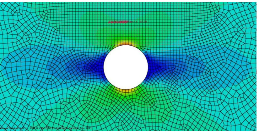
The results of finite element analysis critical to OptiGrating analysis are the strain distribution along the sensors. Despite the slight misalignment of the sensors and the E11 axis, it was decided to continue with using the E11 strain results, rather than maximum resultant strain or any value in between. This will produce minimal error as E11 ranges between 96 and 98.5% of maximum strain across all samples.
Strain distributions from the no defect model were constant along the sensor, while the internal delamination FEA approximated this behaviour. The strain distribution along the sensor embedded in the sample containing a hole appeared to be quadratic. Consequently the data was fitted with a second order polynomial regression using Microsoft Excel. Table 3.11 shows the calculated regressions and the r-squared value. Note that x is expressed in millimetres, and r-squared was consistent for all loads.
Table 3.11- Micro-strain Regressions from FEA
Load (N)
No
Defect
16mm Hole
(A ∙x2 + B ∙x+ C)
Internal
Delamination
A B C
1000 103.3 0.0387 0.2495 110.38 107.63
2000 206.6 0.0774 0.4994 220.76 215.25
3000 309.9 0.1162 0.7484 331.14 322.88
4000 413.2 0.1549 0.9979 441.51 430.51
5000 516.5 0.1936 1.2475 551.59 538.13
6000 619.8 0.2324 1.4969 662.27 645.76
7000 723.1 0.2711 1.7463 772.65 753.39
8000 - 0.3098 1.9958 883.03 -
R-squared 1 0.9994 1
3.5 OptiGrating
This research project aims to find the efficacy of OptiGrating for reproducing and simulating the reflection spectrum of a fibre Bragg grating sensor. The method requires the construction of a virtual FBGS a combination of the manufacturer specification sheet, academic literature and the inverse scattering solver to reconstruct the grating from the reflection spectrum. The inverse scattering solver is only used on the reflection at zero load to create a reference spectrum.
3.5.1 Reconstruction of the Grating from the Reflection Spectrum
The method of reconstructing the grating from the reflection spectrum initially requires several properties of the grating to be specified. A new single fibre must be created with the dimensions and properties of the core and cladding specified. By analysing the known response at zero load from physical testing, the initial Bragg wavelength (central wavelength) is known.
The sensors used in the experimentation were made from SMF (single mode fibre)-28C, a pure silica doped with Germania (positive) and fluorine (negative) and acrylate recoat. The cladding diameter was known as 125μm, while the core diameter was 8.2 μm (Julich & Roths 2009). Central wavelengths were defined as the Bragg wavelength
the cladding refractive index has no impact on the Bragg response (Ashby 2007). The values are displayed in Table 3.12.
Table 3.12- FBGS Properties for OptiGrating
Sample A Sample A1 Sample B
Central Wavelength (μm) 1.548213 1.548115 1.552115
Core Width (μm) 4.1 4.1 4.1
Core Refractive Index 1.44405 1.44405 1.444
Cladding Width (μm) 62.5 62.5 62.5
Cladding Refractive Index 1.3 1.3 1.3
For more accurate replication of the spectra, material dispersion was enabled. The Sellmeier equation is shown by equation 3.1, while the Sellmeier parameters are shown in Table 3.13, and were obtained from the OptiGrating library. This library uses data from Bass et al. (2009) and (I.H.Malitson 1965).
𝑛2 − 1 = 𝐴1 ∙ 𝜆
2
𝜆2 − 𝜆 12
+ 𝐴2 ∙ 𝜆
2
𝜆2 − 𝜆 22
+ 𝐴3 ∙ 𝜆
2
𝜆2 − 𝜆 32
(3.1)
Where;
A1, A2, A3 are the amplitude Sellmeier coefficients
λ1, λ2, λ3 are the wavelength Sellmeier coefficients
Table 3.13- Table of Sellmeier Parameters
Host Dopant + Dopant -
Description Pure Silica Germania-doped Silica Fluorine-doped Silica
A1 0.6961663 0.7028554 0.69325
A2 0.4079426 0.4146307 0.3972
A3 0.897479 0.897454 0.86008
λ1 (μm) 0.0684043 0.0727723 0.06723987
λ2 (μm) 0.1162414 0.11430853 0.11714009
λ3 (μm) 9.896161 9.8961609 9.7760984
After the initial property assignment of the FBGS, the inbuilt inverse scattering solver (ISS) was accessed to reconstruct the grating from the knowledge of the reflection spectrum. The spectrums to be reconstructed were the zero load reflection for each sample.
Table 3.14- Micron Optics Text File Format
Column 1 Column 2 Column 3 Column 4 Column 5
Wavelength (nm) Channel 1 Reflection (dB) Channel 2 Reflection (dB) Channel 3 Reflection (dB) Channel 4 Reflection (dB)
OptiGrating requires the text file to be only two columns. Column 1 must be the wavelength in micrometres (μm), and column two must be the reflection expressed as a power ratio. The relationship between sound pressure level (Lp) and the power ratio (R)