MoL 2010 10: Temporal Binding by Short Term Synaptic Plasticity

Temporal Binding by Short-Term Synaptic

Plasticity

Ernst Odolphi

[email protected]

March 30, 2010

Abstract

This thesis introduces a novel way of performing temporal binding in a network of biologically plausible spiking neurons. The neurons in the

net-work are connected through synapses with short-term synaptic plasticity. By synchronously activating multiple patterns, the network stabilizes into

a state where these multiple patterns quickly oscillate between an active

and inactive state.

Using this method a simple Hopfield-like auto-associative network is

Acknowledgment

I would like to thank everybody who helped my in the writing of this the-sis. Specifically Reinhard Blutner for his supervision, Michiel van

Contents

1 Introduction 5

2 Neural Networks 8

2.1 Classical Neural Networks . . . 9

2.2 Spiking Neural Networks . . . 10

2.3 The Spike Response Model . . . 10

2.3.1 The Model . . . 11

2.3.2 Example . . . 13

2.3.3 Activity in the Spike Response Model . . . 15

3 Auto-associative Networks 16 3.1 Associative Neural Networks . . . 16

3.2 Storing Patterns . . . 17

3.3 Distributed Representation . . . 18

4 Binding Problem 21 4.1 Temporal Binding . . . 22

4.2 Synchronous temporal binding . . . 24

4.2.1 Shruti . . . 24

4.2.2 Neural Oscillators . . . 26

4.2.3 Disadvantages of synchronous binding methods . . . 26

4.3 Slow Temporal Binding . . . 27

5 Temporal Binding by Short-Term Synaptic Plasticity 30 5.1 Pattern Retrieval . . . 30

5.2 Pattern separation . . . 31

5.2.1 Short-Term Synaptic Plasticity . . . 33

5.3 Switching Patterns . . . 36

5.4 Measuring Binding . . . 38

6 Simulations and Results 40 6.1 Simulations . . . 40

6.1.1 Retrieving one pattern . . . 40

6.1.2 Retrieving two patterns . . . 40

6.1.3 More patterns . . . 42

6.2 Results . . . 43

6.2.1 One pattern . . . 43

7 Future Work and Conclusion 49

7.1 Future Work . . . 49

7.1.1 More Realistic Domain . . . 49

7.1.2 Whole/Parts Modeling . . . 49

1

Introduction

Distributed representations in neural networks have a very strong appeal. They are easy to implement and fault tolerant. They generalize, have

a large capacity and are very expressive. There has been quite a lot of research in the relations between logic and these networks.

There are however also some big problems limiting the use and ex-pressive power of neural networks with distributed representations. One

of the biggest problems is the binding problem. It is difficult to represent

more then one object in such a network, since there is no information about which unit belongs to which object.

Several solutions to this problem have been proposed. One solutions that has been given a lot of attention is called “temporal binding”. In

this method of binding, introduced in [von der Malsburg, 1981], the exact timing of the spikes of the neuron is used to indicate which neuron belongs

to which object.

Most research on temporal binding focuses on using exact synchrony

of spikes to signal binding. In these models neurons firing in synchrony are said to “belong” to the same pattern. This way the network activity

quickly oscillates between active patterns. Since the duration of a spike

is between 2 and 10 milliseconds, the network switches patterns approxi-mately every 5 to 20 milliseconds.

[Knoblauch and Palm, 2002] introduces a model that implements tem-poral binding on a much slower time-scale. Instead of neurons firing in

synchrony, neurons are active in short “bursts”. Neurons belonging to the same pattern are active during the same bursts. This means the network

switches patterns on a much slower scale, somewhere between every 50 to 200 milliseconds.

This thesis will introduce a model that implements a variant of this binding method. The resulting binding behavior is similar to that of the

model implemented by [Knoblauch and Palm, 2002]. The model in this

thesis consists of a simple auto-associative network of spiking neurons, universally connected through synapses with short-term plasticity. In

bi-ological neurons the transmission of a spike changes the strength of a synapse. [Kistler and van Hemmen, 1999] introduce a model that

imple-ments this characteristic of synapses and show that short-term synaptic plasticity impacts network behavior, but does not impact the capacity

of auto-associative networks with these synapses. This thesis shows that the short-term synaptic plasticity modeled in [Kistler and van Hemmen,

of [Knoblauch and Palm, 2002].

Whereas in the model of [Knoblauch and Palm, 2002] the binding

behavior is implemented using a complex network consisting of multiple layers, in the proposed method the binding behavior simply emerges from

a straight-forward associative network of spiking neurons which are

con-nected through synapses with short-term plasticity. The binding method does not require any machinery added to the associative network, making

it much simpler than other proposed solutions.

Section 2 gives a general introduction to neural networks. It introduces

central concepts in artificial neural networks, like neurons, synapses and activity.

In biological neural networks, activation is spread through the network by short spikes. Since the exact timing of these spike did not seem to play

an important role in the workings of neural networks, classical artificial neural networks do not model these spikes. Instead the average frequency

of these spikes is modeled.

Since the binding method developed in this thesis uses the exact timing of spikes to perform binding, section 2 introduces a variant of artificial

neural network that does model the spiking nature of neural activity. This section introduces a mathematical model of spiking neurons. Though

more complex than classical neural networks, it remains fairly simple, which allows the paper to focus on the binding method.

Section 3 introduces auto-associative networks. These networks are capable of storing patterns and retrieving the stored patterns by activating

parts of the stored patterns. Patterns are stored by changing the strength

of the synapses connecting the neurons.

This section also shows how information can be encoded in patterns in

an elegant way in neural networks. Nodes in the network represent prop-erties of objects. Objects are represented by a pattern of these propprop-erties,

i.e. the properties that that object has. These patterns can be stored in auto-associative networks and have some very attractive properties.

A problem however with these so-called distributed representations is that only one pattern can be active at the same time. When two patterns

are activated we need a way to keep track of which properties belong to which object. This problem, generally called the binding problem, is

introduced in section 4. Without a solution it seems impossible to model

complex things like relations in distributed representations.

This section also introduces a solution to the binding problem proposed

two models, that use synchrony in spikes to model binding and keep track of which active node belongs to which active pattern. Some problems

with these models are discussed. The section also introduces the model of [Knoblauch and Palm, 2002], where neurons are bound to patterns on

a slower time-scale.

Section 5 introduces a novel way to perform temporal binding in an auto-associative network on a slow time scale similar to that of [Knoblauch

and Palm, 2002]. The binding emerges in a standard auto-associative net-work of spiking neurons with short-term synaptic plasticity from [Kistler

and van Hemmen, 1999]. Short-term plasticity, the fact that synapses fatigue when transmitting spike and thus become less and less effective,

controls the activity in the network, resulting in a temporal binding be-havior but with much less added complexity.

A computer model of the binding method developed in section 5 is used to perform simulations in section 6. A simple network of spiking

neurons is used to retrieve one, two and three patterns simultaneously.

The simulations show that the method can indeed be used to perform binding in a simple network of spiking neurons and short-term plasticity.

Section 7 introduces some aspect of the binding method that might be interesting to the develop in future work, and gives a conclusion to the

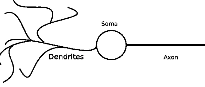
Figure 1: A schematic representation of a biological neuron

2

Neural Networks

Over a hundred years of biological research have given us a lot of insight

in the structure of our brain. This research showed that neurons are the primary processing units in our brain. The brain consists of a huge

number of these neurons connected to each other in a complex network. The estimated number of neurons is about 1012_{. A typical neuron is}

connected to approximately 104other neurons [Maass and Bishop, 1999].

A typical neuron consists of three main parts, see figure 1. The den-drites of a neuron consist of a tree that collects pulses from pre-synaptic neurons, i.e. the neurons which connect to the current neuron. The body of a neuron is called the soma. The incoming pulses collected by the dendrites cause a potential change in the soma. If this potential crosses a threshold, the soma emits a pulse. This pulse is propagated to the

post-synaptic neurons, i.e. the neurons to which the current neuron is connected, by theaxon.

The duration of a pulse is typically 1-2 ms. It is generally assumed that the exact shape and duration of a spike carries no information. Only

the time of a pulse and the number of pulses emitted matter.

The place where the axon of one neuron meets the dendrite of another neuron is called the synapse (hence the term pre- and post-synaptic).

When a pulse of the pre-synaptic neuron reaches this point, a highly complex chain of chemical reactions causes a changes in the potential of

the post-synaptic neuron. The size of the change is determined by the strength of the synapse. The changes can either be positive (the synapse

2.1

Classical Neural Networks

Classical artificial neural networks give a simple mathematical model of

neural networks as described in the previous section. Essentially a network consists of a set of nodes representing the neurons, and a matrix of weights

representing the synapses connecting the neurons.

Each node has an activation value associated with it. This activation

value represents the firing rate of the neuron. The higher the firing rate, the higher the activation of the node.

The reaction depends on the type and strength of the synapse connect-ing neuron iandj. This is modeled by the activation levela of neuron

k depends on the activation level of the pre-synaptic neurons and the

strength of the synapses connecting the pre-synaptic neurons.

The strength of the synapse is models bywij (the weight of the

con-nection from neuron j to neuron i). If wij is positive, the synapse is excitatory. If a neuroni receives input from an excitatory neuron, the

activation level of neuroniwill increase. Ifwijis negative, the synapse is inhibitory. If neuronireceives a spike from an inhibitory neuron the

acti-vation level of the neuron will decrease. The value ofwijdetermines the strength of the synapse. The stronger the synapse the more the activation

level of the neuron will increase or decrease.

The sum of the activation levelaj of the pre-synaptic neuronsj6=k multiplied by the synaptic strengthwjkof the synapses connecting neuron

kandjis usually called the input of the neuron. So the input,skof neuron

kat timet+ 1 is:

sk(t+ 1) =X j6=k

aj(t)wjk (1)

The way the activation level of a neuron depends on it’s input is called

the activation function. Several activation functions are used in artificial neural networks. The simplest activation function is the binary activation

function. Units that have a binary activation function have an activation level of 1 if the input exceeds a certain thresholdT and 0 if the input is

below the thresholdT.

ak(t+ 1) = 1 ifsk(t+ 1)> T,0 otherwise (2)

Another popular activation function is the sigmodial activation

func-tion:

ak(t+ 1) = 1

2.2

Spiking Neural Networks

Classical neural networks as described in section 2.1 give a simple

math-ematical model of networks of neurons. These models allow for empirical and theoretical research. Because mathematically these models are

rel-atively simple, it is possible to make rigorous proofs, such as the one mentioned in 3.1.

One of the simplifications that often proves too strong is the fact that the exact firing times of the neurons are not modeled. In biological neural

networks, the activity is spread through the network by neurons that fire small spikes. In classical neural networks it is assumed that the exact

timing of the spikes carries no meaning.

So to simplify the model, activity in the network is modeled by the ac-tivation level of a neuron, which can roughly be interpreted as the number

of times a neuron fires a spike within a certain time period. Instead of car-rying spikes through the network, the synapses are modeled to transport

these activation levels.

This greatly simplifies the model, however it often proves too much

of a simplification. The binding method developed in this thesis uses the exact timing of spikes to bind neurons to a pattern. So classical models

of artificial neural networks can not be used to implement the binding method.

2.3

The Spike Response Model

In this section I will introduce a precise mathematical model of a network of neurons called the Spike Response Model [Maass and Bishop, 1999].

This model abstracts from the exact biological details of the neurons. In this way the model can be fairly simple. However it is powerful enough

to explain various phenomena of biological neural networks.

The method of binding developed in this thesis uses the exact

tim-ing of spikes to perform bindtim-ing. To implement the bindtim-ing method we thus needs to implement a model of spiking neural networks. The spike

response model is relatively simple to implement while staying relatively

close to biological neurons. The spike response model is also the model chosen in [Kistler and van Hemmen, 1999] to implement short-term

2.3.1 The Model

The state of a neuroniat timetis modeled by the action potentialµi(t)

of that neuron. Whether or not a neuron fires a pulse to its post-synaptic neurons is controlled by this action potential. If the action potential of

neuroni crosses the neuron’s firing thresholdθi the neuron will emit a pulse along it’s axon. So the setFiof firing timesti(the times a neurons

emits a pulse) is defined by the exact times the action potential of the neuron crosses the firing threshold of a neuron:

Fi={tkµi(t) =θi} (4)

There are two processes that contribute to the value of the action

potentialµi of neuron i. First, there is the reaction of a neuron to it’s own pulse, it’s so-called refractoriness, this is modeled by a functionηi(t).

And second, the reaction of a neuron i to pulses of a pre-synaptic neuronj, is modeled byij(t). The potential at timetis determined by

all reactions to it’s own spikes and by all reactions to the spikes of the neuron’s pre-synaptic neurons. I.e.:

ui(t) = X tf∈Fi

ηi(t−tf) +

X

j∈Γi

X

tg∈Fj

ij(t−tg) (5)

where Γi is the set of pre-synaptic neurons of i. The first term of

the right side of equation 5 represents the response ofito it’s own firing,

the second term corresponds toi’s response to firing of it’s pre-synaptic neurons.

After a neuron emits a pulse it cannot emit any pulses for a short while. This phenomena is called absolute refractoriness. After that the

potential µi is lowered to a value below the resting potential µresti , i.e. the value to which the potential of the neuron converges if it receives no

pulses. The lowering of the potential has the effect that it is more difficult for the neuron to fire after emitting a pulse. This phenomena is called

relative refractoriness.

So the reaction of a neuronito it’s own pulse at timescan be modeled by:

ηi(∆t) =

    

−µ_refracexp[−(∆t)/τ] if ∆t≥_∆abs −∞ if 0≤(∆t)<_∆abs

0 if (∆t)<0

(6)

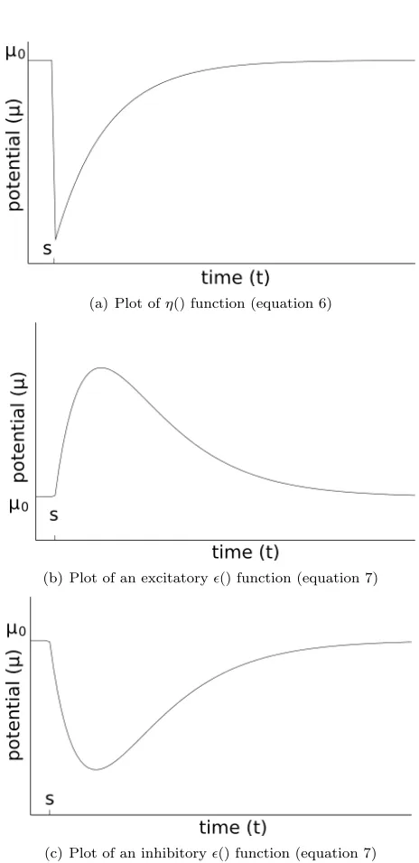
(a) Plot ofη() function (equation 6)

(b) Plot of an excitatory() function (equation 7)

(c) Plot of an inhibitory() function (equation 7)

determining the length of the relative refractory period, and µ_{refrac a}

constant determining the amount the potential is lowered due to a spike.

Figure 2 shows a graph explaining equation 6.

For simplicity I will assume the sameηfor every neuron. [Maass and

Bishop, 1999] uses equation 6 in most parts of the book. It is however

possible to choose a different equation and for example model different types of biological neurons.

If neuron ireceives a pulse from a pre-synaptic neuron j ∈ Γi, this pulse will cause a reaction of the potentialµi of neuroni. The weight of

the synapses determines the direction and magnitude of the reaction. As in the models of classical artificial neural networks in the previous section,

this is modeled bywij.

When a pulse arrives at the neuron, the potential changes rapidly.

After reaching the full potential change the potential will gradually recover to the resting potential. [Maass and Bishop, 1999] models this as:

ij(∆t) =

(

wij[exp[−((∆t)_τ−∆ax

m )]−exp[−(

∆t−∆ax

τs )]] if (∆t)≥∆ ax

0 otherwise

(7) Whereτs andτmare time constants that determine how fast the

po-tential recovers, and where ∆axmodels the axonal delay (i.e. the time it takes for a pulse to reach the post-synaptic neuron).

Again for simplicity I assume the same for every pair of neurons.

Throughout the simulations equation 7 is used to model a neurons reaction to it’s own pulses.

The equations in this section make up the basic structure of spike response model. They completely abstract away from the biological

pro-cesses involved. The model just gives a basic structure of how neurons react to pulses. However it is possible to choose more involved equations

forηandand create a models that more precisely models the chemical processes. For our purpose, a simple model suffices, since the model does

not crucially depend on any of the low-level chemical processes.

2.3.2 Example

Consider the figures 3(b) and 3(c). The figure shows a part of a network

of neurons (figure 3(a). Neuron 1 is connected to neurons in the network

that fire randomly. Neuron 2 is connected to Neuron 1 by an excitatory synapse.

(a) Part of a network of neurons.

(b) Potential of Neuron 1.

(c) Potential of Neuron 2.

At timet= 0 the potential is equal to the resting potentialµrest. Neuron 1 receives excitatory input from other neurons in the network. Every

pulse that is emitted by the pre-synaptic neurons of Neuron 1 causes a change in the potential of the neuron, as modeled by equation 7. At time

t = t1 the potential of of neuron 1 crosses the threshold. This means

that at t1 Neuron 1 fires a pulse as modeled by equation 4. The firing causes a negative contribution to be added to the potential of the neuron

as modeled by equation 6.

Neuron 2 is connected to Neuron 1 through an excitatory synapse.

When the spike reaches the synapse connecting the neurons att1+ ∆axon a positive contribution of () is added to the potential of Neuron 2 as

modeled by equation 7 (figure 3(c)). At times t2 and t3 the potential crosses the threshold again, resulting again in a raising of the potential of

Neuron 2.

2.3.3 Activity in the Spike Response Model

The spike response model introduced above gives a simplified model of

biological neurons. This subsection shows how the spikes emitted by spike

response neurons can be interpreted to resemble the activity of classical neurons (see section 2.1).

The activity of neuron neuroniat timet,ai(t), can be interpreted as the firing rate of the neuron a timet. This is defined as the total number

of pulses a neuron emits over the time intervals[Maass and Bishop, 1999]:

ai(t) =|{tf ∈F|(t−s)< tf < t}| (8)

Using this definition we can describe the state of a network at timetby a vectora(t) ={a1(t), . . . , an(t)}, just like we can represent the activity of a classical network by it’s activity vector.

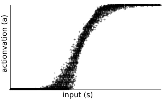
[Gerstner, 1999] shows that the activation function of a spike response

neuron with absolute refractoriness can be modeled by a sigmoidial func-tion. Figure 4 shows a plot of a simulation performed using the model

described above. The input of a neuron is plotted against the average fir-ing rate of the neuron. The plot clearly shows that the activation function

Figure 4: Result of a simulation of a spike response neurons. The figure plots the received input of a neuron against the firing rate of the neuron.

3

Auto-associative Networks

Networks of neurons generally perform a computation by activating neu-rons and letting the activation spread through the network. The activity of

some neurons is raised, and through the excitatory synapses, post-synaptic neurons are activated. They perform a mapping of one set of activation

vectorsx1, x2, . . . , xnto another set of activation vectorsy1, y2, . . . , yn. Two types of mappings can by distinguished. In the first type, the

activation values of one set of neurons are mapped to the activation values of another set of neurons. Such network are called hetero-associative. The

network can also perform a mapping of the activation values of a set of neurons to the activation values of the same set of neurons. These second

type of networks are called auto-associative.

Attractor neural networks are a special type of auto-associative net-works. They consist of universally connected neurons, i.e. every neuron is

synaptically linked to all other neurons in the network. By changing the weights of the synapses, patterns can be stored in the network. If a partial

pattern is activated, the activation spreads through the network activating the rest of the pattern, essentially implementing a type of memory.

3.1

Associative Neural Networks

[Hopfield, 1982] showed that a certain class of neural networks will always

consist of elements described by equations 1 and 2, which are updated asynchronously. This means that at every time t the activation value

of only one (randomly selected) neuron is updated. The elements are connected by symmetrical weights, i.e. the weight connecting neuron i

to neuron j must be the same as the weight connecting neuron j to i,

or more formally: ∀i, j: wij =wji. Hopfield showed that if a group of neurons in such a network is activated the network will always converge

to a stable state.

3.2

Storing Patterns

If the neurons in a network are connected through symmetrical synapses, the network will converge to a stable state after activating certain neurons.

What states are stable depends on the weights of the synapses in the network. By changing these weights it is possible to change the attractor

states in the network.

[Hebb, 1949] introduced a method of changing the strength of a synapse based on the activity of the pre- and post-synaptic neurons of the synapse.

The process of changing the weight of a synapse according to the activity of the neurons it connects is called synaptic plasticity.

Hebb’s idea was that simultaneous activity of two neurons can be in-terpreted as a way of “belonging together” of the two neurons. “Neurons

that fire together wire together”. By increasing the strength of the con-nection between two neurons if they are active together, this information

can be stored in the network. If the connection between the neurons is

strong enough and one of the two neurons is active, the other neuron will be activated because of the strong positive connection between them. The

network has “learned” that the neurons belong together.

This general idea of long-term synaptic plasticity can be used to store

patterns in a network. Patterns are stored by presenting an activation pat-tern to the network, and then adjusting the weights according to Hebb’s

idea about long-term synaptic plasticity. If two neurons belong to the same pattern their connection is strengthened.

The stronger positive connections between two neurons belonging to the same pattern will mean that activation of one of the neurons will

heighten the potential of the other neuron. Looking at the complete

More formally Hebb’s idea can be expressed as

∆wij=γ∗(xixj) (9)

wherexiis the activation of neuroniandγ is usually called the learning rate.

Note that when the activation of the neurons in the presented patterns is positive the weights in the network continue to grow. Often when storing

binary patterns,{−1,1}are used as activation values. This has the effect that besides positive connections, also negative connections are created.

When one of the neurons is active and the other is not, the connection

between the two neurons is weakened instead of strengthened.

3.3

Distributed Representation

In classical computers information is retrieved from memory by finding the exact address of the stored item. If an item has to be retrieved the

exact location of the item in memory has to be computed, which is not necessarily trivial.

The previous subsections showed how a simple network of neurons can be used to implement a content addressable memory. Using a simple rule,

patterns can be stored, and later retrieved by activating a part of that

pattern. There are various ways to store information in such patterns, for this thesis however I will focus on the two most obvious and different

techniques: local representation and distributed representation.

Classical cognitive theory tends to adhere to local representations.

Objects are represented in one place in the system, i.e. a memory address, a node in the network or, from a classical analogy for human memory, a

drawer in a big closet. If information about an object is to be retrieved, first the location of the object is retrieved, from which the information

about the object can then be retrieved.

The auto-associative networks from the previous subsection suggests

a different but elegant way to store objects. Instead of letting the nodes

in a network represent objects, they represent features of that object. An object is represented by an activation vector. Active nodes in the

vec-tor represent features that belong to the object, inactive nodes represent features that do not belong to the object.

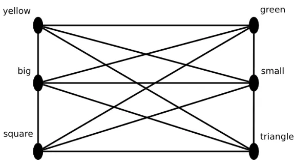
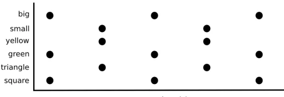
Consider figure 5, it shows a network of 6 nodes. The 2 nodes on the top represent color, the central nodes represent size, and the bottom nodes

Figure 5: Example of a network using a distributed representation

The example above uses binary units (see 2.1). Using analog units would give us an even more expressive network, “where smallish” and

“yellowish” objects can be represented.

Representations similar to the representation in figure 5 are called

distributed representations (see [Rumelhart and McClelland, 1987] for a good overview). The classical types of representation where objects are

represented in one place are called local representations.

Distributed representations have some advantages over local

represen-tations. For one, using local representationsnobjects can be represented

usingnnodes. Using a binary distributed representation 2nobjects can be represented using n nodes, since every different pattern represents a

different object. So a network that uses a distributed representation can represent exponentially more objects than a local representation can.

Using a local representation, representing new objects requires special mechanisms, since new nodes need to be assigned for the new objects.

There are methods for this, however if implemented in a neural network, there has to be some machinery and bookkeeping to do this. In a

dis-tributed representation, new object do not need to be assigned to a node, the object can just be activated by activating the corresponding pattern.

Distributed representations are fault tolerant. If a feature of an object

is misrepresented, the network will usually repair that, because of the feedback from the network. In a local representation this is much more

difficult.

Distributed representations are much more robust then local

4

Binding Problem

The previous section shows how a simple network of neuron-like elements can implement a content-addressable memory, and how these networks

suggest a simple but extremely powerful way to represent objects in a network. Although distributed representations have many nice features,

they also have some severe shortcomings.

One of the biggest problems with distributed representations (see

sec-tion 3.3) in classical neural networks, was pointed out by Frank

Rosen-blatt [RosenRosen-blatt, 1962] using the example from figure 5. The figure shows how configurations of a square and a triangle can by represented using a

distributed representation. A small green triangle is represented by the features (small, green, triangle), a big yellow square is represented by the

features (big, yellow, square).

The problem arises when we want to represent a small green

trian-gleand a big yellow square. This will be represented by (small,green,

triangle, big, yellow, square). A small yellow square and a big green

triangle is represented by (small,green, triangle,big,yellow,square). It is impossible to tell both representations apart, because there is no way

to tell which feature belongs to which object.

In general this problem always arises when more than one object is to be represented using a distributed representation. There has to be a way

to bind features to objects if more than one object has to be represented. This problem is known as the binding problem [von der Malsburg, 1981].

The problem does not only occur if visual information has to be rep-resented in a distributed way, it also occurs if information from different

modalities (i.e. visual and auditive) has to integrated into one object. The next sections introduces a solution to the binding problem as

pro-posed in [von der Malsburg, 1981]. This method uses the exact timing of spikes in a network of neurons to perform binding. Three implementations

of this method are discussed in the following couple of sections. Section 5

develops a novel way to perform temporal binding, where temporal bind-ing emerges from the use of short-term synaptic plasticity. The proposed

method is both more biologically plausible and less complex, in the sense that it can be implemented in a simple network of fully connected spike

re-sponse neuron, without the need for complex neuronal units or a complex network structure.

Various other solutions have been proposed to solve the binding prob-lem. [Smolensky, 1990] proposes a mathematical solution called tensor

of both objects and variables, and represents the binding using the tensor product of the two.

Another proposed solution is that the problem is solved hierarchically. The world is represented in successively more complex representations.

Nodes in the layers of higher complexity represent more and more specific

things, making it possible to distinguish objects from each other. Recently temporal solutions of binding have received a lot of attention

(see for example the special issue of Neuron on binding: [Shadlen and Movshon, 1999], [Roskies, 1999]) for example), and various solutions have

been proposed. The general idea of using spike times for binding seems very elegant and simple. However most of the proposed models that

per-form binding this way tend to be complex, or have various other problems that limit the elegance and representational power of these models (see

section 4.2.3). This thesis develops a model of temporal binding which uses short-term synaptic plasticity to implement slow temporal binding.

4.1

Temporal Binding

This thesis focuses on temporal binding, as introduced in [von der Mals-burg, 1981]. There it is noted that the exact timing of spikes which is

usually considered without meaning in classical neural network could be used to implement binding.

[von der Malsburg, 1981] proposes to use the exact timing of the spikes for binding, hence the name temporal binding. A visual illustration of this

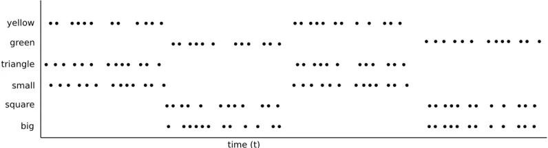
idea, makes it clear how this works. Consider figure 6, which shows firing

times for the neurons from figure 5. Note that the firing rate, and thus the activation level of all the neurons is equal. When looking only at the firing

rate we have a similar pattern as before, all neurons are active, making it impossible to tell if this represents “a large green triangle and a small

yellow square” or “a large yellow triangle and a small green square”. When looking at the exact firing times however it is possible to see

what is represented. The spikes for “large”, “green” and “square” are always synchronous, as are the spikes for “small”, “yellow” and “triangle”.

The exact timing of the spikes make it possible to bind patterns of neurons to objects, making it possible to represent more than one object at the

same time.

[von der Malsburg, 1981] notes that this synchronicity is almost cer-tainly unconscious. People are not capable of consciously perceiving

Figure 6: Binding through synchronous firing. Network activity of a network representing a small yellow triangle and a big green square. Each dot repre-sents a particular neuron firing a pulse. The fact that the neurons representing the features “small”, “yellow” “and triangle” fire in synchrony indicates that they are features of the same object. This synchrony “binds” the neurons to-gether. Note that the same holds for the neurons representing “big”, “green” and “square”.

somewhere between 200ms and 500 ms, so the synchrony of the neurons

would not be something that is consciously perceived.

The duration of the psychological moment is much longer than the du-ration of a single spike, making it possible to implement temporal binding

using other methods than exact synchrony. Short burst of activity as depicted in figure 7 are also possible, for example.

Section 4.3 shows a model that implements this type of binding. This thesis develops a novel way of implementing this slow temporal binding

using short-term synaptic plasticity (See section 5).

One of the things to notice is that although more than one pattern can

be distinguished using this method, the number of different patterns re-mains small. The more different patterns are active the closer the timings

of the spike come together. Since the timings of the spikes of the neurons

are inherently noisy, the upper limit is probably rather low.

Various researchers ([von der Malsburg, 1981], [Shastri and

Ajjana-gadd, 1993] for example) have argued that this is possibly in accordance with studies from cognitive psychology. People are not capable of focusing

on more than a handful of objects at the same time, and most people can not keep more than about 6 words in active memory. This would mean

that this low and hard barrier on simultaneous representation does not have to be a problem.

Figure 7: Binding through bursts of activation. Network activity of a network representing a small yellow triangle and a big green square. Neurons are not bound by synchrony of the spikes. Instead, the neurons belonging to one pattern are simultaneously active in short burst. Since the length of the bursts is still much lower than the psychological moment, the changes in activation will still be unconscious.

(or scenes) consisting of more than one object. In fact most methods of

temporal binding do not offer a way to store scenes of objects (except for the method in section 4.2.1).

4.2

Synchronous temporal binding

There has been a lot of research into the possible implementation of

tem-poral binding in spiking neural networks using synchronous pulses. This section will introduce two of the more prominent models. After this, some

disadvantages of these models are discussed.

4.2.1 Shruti

Lokendra Shastri [Shastri and Ajjanagadd, 1993], implements “a

connec-tionist model of knowledge representation and reflexive reasoning”

in-spired by the ideas on temporal binding from [von der Malsburg, 1981]. In this work a network of simple processing units is constructed, that can,

in a distributed manner, perform reasoning tasks. Binding is achieved by explicitly synchronizing firing times of nodes in the network.

[Blutner and Doherty, 1997] shows that associative networks imple-ment a form of non-monotonic logic. Without binding however, the

ex-pressive power of these models is severely limited. To represent a state-ment like “John loves Mary” in a distributed fashion there has to be a

[Shastri and Ajjanagadd, 1993] represents relations such as “John loves Mary”, by synchronous firing of the nodes john and lover, and

syn-chronous firing of the nodes mary and beloved, and thus binding the nodes forjohnandloverto the same object, and simultaneously binding

the nodes formaryandbelovedto another object.

To achieve this Shastri et al. introducep-btu nodes andτ-and nodes. Both these types of nodes are simple neuron-like processing units that fire

pulses to connected nodes. They however have some special properties that makes it possible to control the synchronization of the firing times of

nodes.

p-btu nodes behave as follows:

• If a nodeAis connected to nodeB, the activity of nodeB synchro-nizes with the activity of nodeA.

• The periodic activity of nodeAleads to synchronous periodic activ-ity in nodeB within one period.

• A threshold,n, associated with a node indicates that the node will fire only if it receivesnor more synchronous inputs.

In this way p-btu nodes can form chains of synchronous firing. In

[Shastri and Ajjanagadd, 1993] this is used to encode rules. The nodes are used to implement the synchronization between roles (arguments of a

predicate) and fillers (objects that fill these predicate arguments) and of arguments of the antecedent predicates to the arguments of the consequent

predicates. In this way it is possible to implement simple first-order like rules, in a distributed way.

τ-nodes behave as follows:

• A τ-and node becomes active if it receives an uninterrupted pulse train, i.e. it receives pulses such that the gap between pulses is less that a pulse width.

• So aτ-and node receiving periodic pulses with periodπ produce a periodic pulse with periodπ.

• A threshold,n, associated with aτ-and node indicates that the node will only fire if it receives more thannpulses within the length of a pulse.

τ-and nodes make it possible to encode facts. This is done by creating

[Shastri and Ajjanagadd, 1993] shows how a network of these two types of nodes can perform various reasoning and query-answering task

by encoding facts and rules in a network of these nodes and activating the network in a way that represents a question.

4.2.2 Neural Oscillators

[Ursino et al., 2006] constructs a network of biologically plausible spiking neurons that perform binding using synchronous firing.

A network of neural oscillators is constructed. An oscillator is formed

by coupling an inhibitory neuron with an excitatory neuron. Activating the excitatory neuron will result in periodic firing of the excitatory neuron

due to the feedback of the inhibitory neuron. These neural oscillators are called Wilson-Cowan oscillators.

An associative network is constructed by connecting the excitatory neurons in the oscillator. Patterns can be stored in this network by basic

Hebbian learning. When two oscillators are connected, a positive connec-tion (i.e. excitatory synapses) favors synchronizaconnec-tion, whereas a negative

connection (i.e. inhibitory synapses) favors de-synchronization.

An inhibitory layer is used to make sure that only approximately one pattern can be active. This, together with the

synchronization/de-synchronization behavior of the oscillators, achieves a segregation of the input.

Shortly after the activation of more than one pattern, the pulses of the neurons belonging to the same pattern synchronize, whereas pulses of

neurons belonging to different patterns desynchronize, effectively binding neurons to the pattern.

4.2.3 Disadvantages of synchronous binding methods

The nodes in the model of [Shastri and Ajjanagadd, 1993] are “Neuron like”, in the sense that they are simple processing nodes connected to

each other in a network. It is however hard to see how these nodes will be constructed from more biologically realistic neural units. Biological units

are noisy and imprecise and do not seem to have mechanisms for explicit

synchronization.

This makes it difficult to see how the model of [Shastri and Ajjanagadd,

1993] could be implemented in a biological system.

The units in the model of [Ursino et al., 2006] are much closer to

form an oscillator. These constructions might be found but do not seem to be ubiquitous enough to facilitate binding on a large scale.

Besides these problems with biological realization of these models, models that use exact synchrony, are argued to be biologically

implau-sible in general. [Shadlen and Movshon, 1999] argues that analysis of

biological brain activity shows that there is not enough correlation be-tween firing times of neurons for temporal synchrony of neurons to play a

role in binding.

A very compelling feature of distributed representations is that the

activation level (i.e. the firing rate) of a neuron signals the strength of the feature in the represented object. I.e. the more active the neuron

encoding the feature “red” is, the redder the represented object is. This rate coding makes distributed representations highly expressive.

In most model of synchronous temporal binding it is not possible for active neurons to have a different firing rate. Either neurons are active

and continuously fire in synchrony or they are not active at all. This

makes rate coding effectively impossible.

Another problem with synchronous temporal binding related to this

is that the refractoring period of neurons make it impossible for a neu-ron to fire immediately after firing. This plays an essential role in the

synchronization in the model of [Ursino et al., 2006] and other models. However this also makes it impossible for a neuron to reliably be active

in more than one pattern. A neuron can only be active in one pattern, making it much more complex to represent two different but similar

ob-jects. It is not clear how to activate more than one overlapping pattern

at the same time.

4.3

Slow Temporal Binding

[Knoblauch and Palm, 2002] implements temporal binding, but on a dif-ferent time-scale. The network in the model consist of two areas. A

peripheral area P, which models the visual cortex and a more central areaCwhich acts as an associative memory, receiving input from areaP.

AreaP models the visual cortex receiving an image as input. Neigh-boring neurons in this section are inhibitorily connected, whereas neurons

further apart are excitatorily connected. This has the effect that area

separates distinct visual object from the input. Neurons representing the same pattern will fire synchronously, effectively binding neurons in this

area to visual pattern.

Figure 8: Topology of the network that implements the segmentation and re-trieval. Adapted from [Knoblauch and Palm, 2002]

Different visual shapes are separated into different patterns. Fire time synchrony is used to indicate which neuron belong to which pattern in

the segmentation.

AreaP serves as input for area C. This area is connected through

Hebbian learning, i.e. it is an associative memory. The patterns that are stored represent visual patterns presented to areaP. When a partial

pattern is activated in area C, the retrieval process of the associative

network will retrieve the full pattern.

If two overlapping patterns are activated in areaP, these visual

pat-terns are separated through the synaptic connections in this area. The activation in areaP is spread to areaC starting a retrieval process for

the full pattern that are stored in this area.

The neurons in areaCare not bound through synchronous firing

how-ever. The associative areaCis connected to two other areas that together govern the binding process (see figure 8).

AreaCs, the separation area, is activated through areaC, and gives inhibitory input to area C. It inhibits all neurons not belonging to the

current pattern. This has the effect that only one pattern can be active

at the same time. When more than one pattern is active, a process of competition makes sure only one pattern remains active.

the other patterns in the network, areaCt inhibits areaCunspecifically. It also works on a much slower scale. After a period of activity in areaC,

areaCtterminates the activity.

The interaction of the three areasC, Cs_{, andC}t _{has the effect that}

only one pattern is active at the same time in areaC, and that a pattern

remains only active for a short period.

The resulting network behavior in area C (the associative area) is

similar to that of figure 7. One of the retrieved patterns is active for a short period untilCt _{terminates that pattern’s activity, another pattern}

takes over and is again active until areaCt terminates it’s activity again. This way the network continually switches between patterns, with each

pattern active for a short amount of time. So the network binds neurons to patterns using time, but on a much slower scale.

The periods of activity are much smaller than the psychological mo-ment, making the switches between pattern unconscious. [von der

Mals-burg, 1981] already indicates that this type of temporal binding would

also be a valid form of temporal binding.

Note that crossover of neurons between patterns is much more unlikely

in this model than in models of synchronous binding. It is also no problem for neurons to be active in more than one pattern at the same time.

The next section introduces a novel method of implementing this slow temporal binding. Instead of having a series of layers that implement the

pattern switching, the model in the next section the binding emerges in a simple auto-associative network with short-term synaptic plasticity as

5

Temporal Binding by Short-Term

Synap-tic PlasSynap-ticity

Section 3 showed how networks of neurons can be used to implement an

associative memory.

This section aims to implement an auto-associative network that can

retrieve more than one pattern at the same time. Section 4 showed how having more than one pattern active in the network poses a problem,

be-cause it becomes unclear which neurons belong to which pattern. The

same problem arises when patterns are activated. If patterns of fifty neu-rons are stored in a network of hundred neuneu-rons, and two non-overlapping

patterns are to be activated, this has the effect that all the neurons in the network are activated. There has to be a way to bind activated neurons

to their pattern

Section 4.1 showed a method of binding neurons to a pattern by using

time as an extra dimension. Neurons that fire in phase belong to the same pattern, whereas neurons that fire in a different phase belong to a

different pattern, see also figure 6. Section 4.3 showed a method that uses

a slow version of temporal binding, where neurons belonging to the same pattern fire in simultaneous bursts.

This section introduces a novel method of binding that uses short-term plasticity to achieve temporal binding on a time-scale similar to

[Knoblauch and Palm, 2002]. An associative network of spike response neurons is constructed from which multiple patterns can be retrieved

si-multaneously. The resulting network behavior is similar to the behavior of the network developed by [Knoblauch and Palm, 2002], however the

network consists of one simple layer of neurons that are trained using standard Hebbian learning. This model implements slow temporal

bind-ing in a simple Hopfield-like network of spike response neurons. The model

does not suffer from the general problems models of synchronous binding suffer from (as explained in section 4.2.3). The network topology of the

model is much simpler than the model proposed by [Knoblauch and Palm, 2002].

5.1

Pattern Retrieval

Section 3 showed how a network of neurons can be used to store and

retrieve patterns. Patterns are retrieved from the network by activating part of the pattern. In a network of classical neurons these neurons are

[Sommer, 2001] implements such an auto-associative network using a network of spike response neurons. Retrieving a pattern in such a network

is a little bit more complicated, since neurons can be activated in various ways.

One way is to simulate pulses from neurons outside the network, i.e.

activating neurons is done by sending pulses to the neuron, similar to pulses it receives from neurons inside the network. The exact timing of

these pulses can be used to group the activated neurons together in a similar way to the binding solution of [von der Malsburg, 1981].

[Maass and Bishop, 1999] notes that pulses arriving close together have a bigger effect on a neuron’s potential then spikes arriving far apart.

Figure 9 shows the effect on the potential of two pulses arriving close together (a) and two pulse arriving further apart (b). The maximum of

the potential of the neuron is much higher in figure 9 (a) than in figure 9 (b)).

The fact that pulses close together have a bigger effect on the potential

of a neuron can be used to bind activated neurons to a pattern. If the neurons of one pattern are activated by pulses that arrive simultaneously

to all activated neuron belonging to that specific pattern, the potential of these neurons will cross the threshold at an almost equal time. Because

the activated neurons belonging to one pattern fire close together they have a much bigger effect on the potential of their post-synaptic neurons.

Neurons belonging to different patterns will not cross their threshold si-multaneously and thus have a much smaller effect on the potential of their

post-synaptic neurons.

5.2

Pattern separation

As mentioned in section 3.2 the Hebb rule (equation 9), can be used to

store patterns in a network of universally connected neurons. Using this rule, patterns can be stored by (locally) changing the synaptic strength

between neurons.

For simplicity we only look at binary patterns in this thesis. When

presenting the pattern to the network as values in{0,1}, the result will be that with each stored pattern, the strength of the synapses will increase.

When part of a pattern is activated, the excitatory connections will

activate the remainder of the pattern, thus retrieving the full pattern. When two partial patterns are activated, the excitatory connections

usu-ally activate the superposition of both patterns.

be-(a) Plot of the potential of a spike response neuron receiving two pulses close together

(b) Plot of the potential of the same spike response neuron re-ceiving two pulses further apart

Figure 9: Plots of the potential of two neurons. Neuron 1 receives two pulse (s1,

sides positive connections, negative connections will be created between neurons from different patterns. When a partial pattern is activated in

the network the excitatory connections still retrieve the full pattern. When two partial patterns are simultaneously presented to the

net-work, the negative connections between the two patterns will make sure

the network stabilizes to a state where only one pattern is active. This form of competition is used in the proposed binding method to make sure

there is only one pattern active at any moment in time.

Note that this active pattern need not be a completion of one of the

two partial patterns. There might be more than two partial patterns in the superposition of both activated partial patterns.

However, as described in the previous section, by synchronously ac-tivating neurons belonging to the same partial pattern, one of the two

activated partial patterns has a much better chance at becoming the re-trieved pattern than any of the possible spurious patterns in the

superpo-sition of the two partial patterns, since, as the previous section explained,

the effect of simultaneous pulses is much bigger than non-simultaneous pulses.

The combination of the inhibitory connections created when storing patterns and the synchronous activation of patterns makes sure that only

one of the activated patterns can be retrieved at any moment in time.

5.2.1 Short-Term Synaptic Plasticity

Section 3 described how the strengths of synapses can be changed to store

patterns in a network of neurons. This type of synaptic plasticity was described in [Hebb, 1949]. It takes places on a long timescale, from seconds

to even hours. For modeling retrieval from the network, the synaptic strengths are actually assumed to be constant.

[Kistler and van Hemmen, 1999] describes an extension of the spike

response model where a different type of plasticity can be modeled. This type of plasticity takes places on a much shorter time-scale, approximately

on the time-scale of normal network activity. This type of synaptic plas-ticity is called short-term synaptic plasplas-ticity.

Besides the differences in time-scales, there is also a difference in what influences the synaptic strength. In long-term plasticity, the synaptic

strength is influenced by both the pre-synaptic, and post-synaptic neu-ron’s activity. If both neuron are simultaneously active the synapse is

With short-term plasticity the strength of the synapses is only influ-enced by the activity of the pre-synaptic neuron. The general idea is that

transmitting a spike from the pre-synaptic neuron to the post-synaptic neuron takes up some kind of “resource” ([Kistler and van Hemmen, 1999],

section 2), i.e. by transferring the spike across the synapses, chemicals and

energy is used. The use of these resources results in a temporary change of synaptic strength. Either the synapse is weakened, which is called

short-term depression, or the synapse is strengthened which is called short-short-term facilitation. After a spike is transmitted, the resources are recollected, and

the synaptic strength goes back to it’s original value.

[Kistler and van Hemmen, 1999] models both short-term depression

and short-term facilitation. Here I will focus on short-term depression, as only this is relevant for this thesis.

In the spike response model the potential of a neuron is modeled by equation 7. In this equationwijmodels the synaptic strength. [Kistler and

van Hemmen, 1999] proposes to replace the constantswijwith functions

wij(t):

wij(t) =w0ijZij(t) (10)

Where Z(t) can be interpreted as the amount of resource available

at the synapse at timet. Each transmitted spike lowers this amount of resources with a certain amount r. After the spike is transmitted the

resource is recollected. So the amount of resourceRij taken by a trans-mitted spike since the moment of the spike can be modelled as:

Rij(∆t) =

(

rexp[−(∆t)/τ] if (∆t)≥0

0 otherwise (11)

A subsequent spike lowers the amount of resources again withr until the resource is fully depleted. This yields the following equation for the

amount of resourcesZijat timet.

Zij(t) =max({0,1− X

tf∈Fi

Rij(t−tf)}) (12)

whereFi

Figure 10 shows the effect of short-term synaptic plasticity on the strength of a synapse. After the synapse has carried a spike, it’s strength is

decreased. Another spike decreases the strength of the synapse even more.

After the spikes are transmitted, the strength of the synapse recovers to it’s original value.

plas-Figure 10: Plot of the synaptic strength of a synapse carrying a pulse

ticity on associative memory. They conclude that

. . . associative memory networks with synaptic depression are

capable of carrying out their functions, although with a lower capacity ([Bibitchkov et al., 2002], 334)

and

The problem of lower storage capacity for networks with

de-pression can be relieved if one requires just a certain time win-dow for a stable activity in a pattern instead of sustained

ac-tivity ([Bibitchkov et al., 2002], 334).

If an associative memory is created with short-term depressing synapses,

the network retrieves the same patterns as a network with static synapses.

When a pattern is retrieved however, the patterns become more and more susceptible to noise, and the patterns become unstable, retrieving spurious

patterns.

When the network performs slow temporal binding, the long term

stability is not very interesting. Patterns are meant to stay stable for a short while.

[Bibitchkov et al., 2002] shows that associative networks with short-term depressing synapses exhibit a novel behavior where the network

quickly switches from one pattern to another, due to noise. The synapses connected to the active neurons in the pattern become weaker and weaker

due to their reducing resources. The decreasing strength of the active

reaction of neurons to the noise increases.

This behavior of pattern switching will be used in the next section to

implement binding in an associative network that can retrieve more than one pattern at the same time.

5.3

Switching Patterns

Using the techniques described in the previous two subsections, it is pos-sible to implement an auto-associative network of spike response neurons,

that can retrieve more than one pattern simultaneously.

Patterns are stored using Hebbian learning (see equation 9). The

inhibitory synapse makes sure only one pattern can be active at any mo-ment in time as explained in section 5.2. Patterns are activated using the

method described in section 5.1.

The neurons are connected by short-term depressing synapses. When

one pattern is active in the network the strength of the post-synaptic

synapses of the neurons belonging to the pattern is decreased. [Bibitchkov et al., 2002] shows that the network will tend to switch to another pattern

if the strength of the synapses gets low enough. In [Bibitchkov et al., 2002] this switch was induced through noise, and the network would switch to

an random pattern. If more than one pattern is activated, the network will however switch to one of the suppressed patterns.

If a pattern has been active for a while, the post-synaptic synapses of the neurons belonging to the active pattern will be very weak due to

con-tinuous short-term depression. The strength of the post-synaptic synapses

of the neurons belonging to one of the suppressed patterns will be high, as they will be fully recovered because they have been suppressed for a while.

So the active pattern hardly suppresses the other patterns any more due to the weakened inhibitory synapses. The suppressed neurons will strongly

excite neurons in their pattern and strongly suppress neurons in the other patterns. A new competition is started between the suppressed patterns.

One pattern will win and suppress the other patterns, until the synapses are weakened again and a following competition is started.

Figure 11 shows a network where two patterns are activated in an auto-associative network. At first, the red pattern is active, and suppresses the

green pattern. The strength of the active synapses decreases, lowering the

suppression of the green pattern. The synapses of the green pattern are fully recovered, so once the suppression of the green pattern is sufficiently

Using the techniques from the previous section it is possible to im-plement a network that retrieves more than one pattern and binding the

neurons to a pattern using temporal binding as suggested by [von der Malsburg, 1981], however not on the scale of single spike, but on the scale

of a couple of spikes.

Note that it is actually possible to changes the time-scale on which the binding is performed by manipulating the strength of the short-term

plasticity.

5.4

Measuring Binding

Section 5.3 shows how to implement an auto-associative network that can retrieve more than one pattern at the same time. Neurons are bound to

patterns by short periods of activity using short-term-plasticity.

This section shows a method to measure to which patterns a neuron

belongs. Intuitively, neurons that are active in a period belong to the same

pattern. A neuron that is continuously active belongs to all patterns, and a neuron that is not active at all belongs to no pattern. Figure 11 clearly

shows two groups of neurons that are bound using temporal binding. Some neurons are active in the first 120 milliseconds, some neurons are active

in the second 120 milliseconds and so forth.

However if we want to do experiments or simulations we need a formal

definition of when a neuron is bound to a pattern. In other words, we need a definition of when neurons are active together, and when neurons

are not active together.

Activity of a neuron is measured by it’s firing rate (see equation 8). An active neuron has a high firing rate, whereas a inactive neuron has a

low firing rate.

One way to measure the relation of the firing rate of two neurons is

by measuring the the covariance of the firing rate of the neurons. The covariance of the firing rate of two neurons is expressed by equation 13

covr1(t)r2(t)=E(r1(t)r2(t))−E(r1(t))E(r2(t)) (13) Covariance measures the relatedness of the two firing rates. If both

firing rates are high and low at the same times, the covariance is high. If the firing rate of one neuron is high when the firing rate of the other is

low the covariance is low.

If neurons are bound using the technique described in the previous sections, the firing rate of a neuron will go up and down as the pattern

same pattern, they will go up and down around the same times. The covariance of their firing rates will thus be high. If neurons do not belong

to the same pattern the opposite will be true, and the covariance will be low.

One problem with measuring binding this way is that it fails if a neuron

belongs to two active patterns. The neuron will then be active in more than one period. It’s firing rate will not match with the firing rate of any

of the other neurons, however intuitively it should belong to two patterns A high covariance indicates that neurons belong to thesamepattern, however a low covariance does not indicate that the neurons belong to adifferent pattern. So covariance cannot be a decisive measure for slow temporal binding.

Intuitively, neuronnbelongs to the same patterns as neuronmif the

firing rate ofnis high when the firing rate of neuronmhigh. Conversely neuronmbelongs to the same patterns as neuronnif the firing rate ofmis

high when the firing rate ofnis high. If during a period the firing rate ofn

is high, but the firing rate ofmis low, this does not indicate anything with regard to binding, since neuronnmight be active in multiple patterns.

Sorn(t) 0 andrm(t)0 can be taken as an indication that the neurons belong together. We can thus define therelatedness B ofn and

mas

B(n, m) =X t

rn(t)rm(t) (14)

where rn(t) is the firing rate of neuron n at time t. Neuron n and m

6

Simulations and Results

6.1

Simulations

I implemented the model of temporal binding developed in the previous section in C++ (see http://github.com/eodolphi/Spiking to download the

code). This section shows some experimental results from running this implementation. The implementation creates a network of 100 spike

re-sponse neurons (See section 2.3), withτm = 4, τs = 2;τr = 2,∆abs = 2 and a threshold of 0.2.

These neurons are universally connected through synapses with short-term plasticity (See section 5.2.1).

Patterns are stored using the Hebbian learning rule from equation 9. 20 patterns of 10 neurons are stored in the network of 100 neurons.

Pat-terns are retrieved by simultaneously activating 5 neurons from a pattern

using the method described in section 5.1.

This network setup is used in the next three sections to retrieve one,

two and three simultaneous patterns.

6.1.1 Retrieving one pattern

Figure 12 shows the activation of the neurons in the network, when 5

neurons of one of the patterns are activated by simultaneous pulses. The other neurons belonging to the pattern are immediately retrieved. When

the synapses become fatigued, the strength of the synapses becomes lower and the retrieved neurons become inactive again.

This confirms the result of [Bibitchkov et al., 2002]. Note that in this case the activity just dies out. In other case spurious patterns might be

retrieved.

6.1.2 Retrieving two patterns

Figure 13 shows what happens if two patterns are retrieved

simultane-ously. The inhibiting connections between the two patterns ensure that

only one pattern can be active at the same time. The depressed synapses however make the active pattern unstable after a certain period of activity.

At this time the other pattern will take over and become active. The instability encountered in the previous section with one pattern, causes

the other pattern to become active.

When the synapses of the neurons in the second pattern become

Figure 12: Results of a simulation with one active pattern, r=.01, τr = 100.

Repeated from figure 11.

Figure 13: Results of a simulation with two active patterns,r=.02, τr= 50.

Figure 14: Results of a simulation with two active patterns, r=.04,τr= 50.

Figure 14 shows the behavior of a network with a higherr(see equation 11), i.e. the carrying of a spike causes a bigger reaction in the synaptic

strength. So it takes less time for the synaptic strength of the active pattern to be lowered enough for the suppressed pattern to take over.

This has the effect that the periods of activity become shorter.

When the period of activation becomes too low, the patterns do not stabilize any more.

6.1.3 More patterns

When the number of active patterns is increased further, the retrieval becomes gradually worse. Figure 15 show how the network behaves when

three patterns are simultaneously activated. Note that the three patterns are again active in distinct periods. However around 550 ms two neurons

from the red pattern are active during the activity of the green pattern. The moment an active pattern fatigues, the two other patterns

Figure 15: Results of a simulation with three active patterns

6.2

Results

The previous section showed some simulations of a spike response network that retreives one, two and three pattern simultaneously. The plots of the

network activity show that the network binds neurons to their pattern by slow temporal binding.

This section analyzes the retrieval performance of the network when retrieving one, two, and three patterns.

6.2.1 One pattern

[Bibitchkov et al., 2002] shows that the capacity of an auto-associative network is not affected by short-term synaptic plasticity. However, the

stability of the retrieved pattern is affected. When a partial pattern is activated, the activation will spread and activate the full pattern just as in normal auto-associative networks.

The synapses connecting the neurons in the pattern quickly weaken because of the short-term plasticity, which makes the retrieved pattern

unstable. With the synapses connecting the stored pattern weakened, noise and the now relatively strong other synapses will have the effect