Noise suppression using local acceleration feedback control of an active absorber

(1)

This is a repository copy of Noise suppression using local acceleration feedback control of an active absorber.

White Rose Research Online URL for this paper: http://eprints.whiterose.ac.uk/92441/

Version: Accepted Version

Article:

Pelegrinis, M.T., Pope, S.A., Zazas, I. et al. (1 more author) (2015) Noise suppression using local acceleration feedback control of an active absorber. Proceedings of the Institution of Mechanical Engineers, Part I: Journal of Systems and Control Engineering, 229 (6). 495 - 505. ISSN 0959-6518

https://doi.org/10.1177/0959651815573123

Reuse

Unless indicated otherwise, fulltext items are protected by copyright with all rights reserved. The copyright exception in section 29 of the Copyright, Designs and Patents Act 1988 allows the making of a single copy solely for the purpose of non-commercial research or private study within the limits of fair dealing. The publisher or other rights-holder may allow further reproduction and re-use of this version - refer to the White Rose Research Online record for this item. Where records identify the publisher as the copyright holder, users can verify any specific terms of use on the publisher’s website.

Takedown

If you consider content in White Rose Research Online to be in breach of UK law, please notify us by

(2)

Noise suppression using local acceleration feedback

control of an active absorber

Michail T. Pelegrinis, Simon Pope, Ilias Zazas and Steve Daley

22nd December 2014

Abstract

A popular approach for Active Noise Control (ANC) problems has been the use of the adaptive Filtered-X Least Mean Squares (FxLMS) algorithm. A funda-mental problem with feedforward design is that it requires both reference and error sensors. In order to reduce the size, cost and physical complexity of the control system a feedback controller can be utilised. In contrast with FxLMS a feedback controller utilises local acceleration measurements of a sound-absorbing surface instead of global pressure measurements. Most control problems, including ANC, can be formulated in the General Control Conguration (GCC) architecture. This type of architecture allows for the systematic representation of the process and

simplies the design of a vast number of controllers that includeH∞andH2

con-trollers. Such controllers are considered ideal candidates for ANC problems as

they can combine near optimal performance with good robustness characteristics.

This paper investigates the problem of reected noise suppression in acoustic ducts

(3)

controlling locally the reecting boundary structure, a global cancellation of the

undesired noise can be accomplished. In the paper the H2 local feedback control

strategy and performance are investigated using an experimental pulse tube. The

H2 design was chosen because it was able to provide consistently a stable response

in contrast to the H∞ design.

I Introduction

As an increased number of large industrial equipment such as engines, blowers, fans, transformers and compressors are in use, acoustic noise problems become more and more evident [1, 2]. Traditionally, the use of passive techniques has been the method of attenuating undesired acoustic sound waves with enclosures, barriers and silencers. The main problem that occurs when using passive control techniques is the limited eciency at low frequencies therefore the use of active noise control (ANC) in order to reduce sound levels has been investigated thoroughly by the scientic community, particularly for acoustic ducts, and a large number of control schemes have been proposed [1]. Due to the fact that reecting sound waves are a key contributor in acoustic resonances, this paper focuses on noise suppression through the reduction of the reected sound wave in an experimental pulse tube, gure 1.

(4)

implement and also generate signicant measurement noise. In this paper a control scheme that is simple to implement and is focussed on using local measurements in contrast to the remote error microphone required in FxLMS designs is proposed. In order to achieve a reduction in the reection of sound the approach here is to directly control the dynamics of the terminating boundary surface inside the acoustic duct.

Recent work in the eld of ANC has been focused on designing actuator set-ups that will enable active structural acoustic control (ASAC) of low frequency noise radiated by vibrating structures [4]. The work described by these authors explores the development of thin panels that can be controlled electronically so as to provide surfaces with desired reection coecients. Such panels can be used as either perfect reectors or absorbers. The development of the control system is based on the use of wave separation algorithms that separate incident sound from reected sound. The reected sound is then controlled to desired levels. The incident sound is used as an acoustic reference for feedforward control and has the important property of being isolated from the action of the control system speaker. The suggested control procedure makes use of a half-power FxLMS algorithm and therefore requires installation of microphones in order to be applicable and the use of low pass lters, which adds signicant complexity to the solution of the primary problem.

(5)

and will thereby reduce the acoustic radiation eciency. A more rened control design approach in the eld of ASAC is to implement a H2 multi-variable feedback control design [6]. In this work, an array of collocated piezoelectric sensor-actuators are utilised in order to reduce the total radiated sound power of a simply supported thin plate. The main problem when implementing this type of control is the fact that the thin plate used to suppress the noise is not an ecient sound generating device and therefore will have signicant performance limitations (noise reduction).

Another approach found in the literature considers aH∞ control strategy as part of

a hybrid feedforward - feedback control design [7]. This approach combines the benets of both previous mentioned designs (FxLMS and ASAC). The problem of this strategy the high resource demand due to the feedforward controller. Furthermore, contrast to the ASAC design the H∞ feedback design requires global measurements of the plant

(error microphone signal) which increases the implementation complexity signicantly.

Finally, an important application of ANC with the aim of developing ideal absorbers should be mentioned. Specically, the work focuses on how to transform a loudspeaker in an active electroacoustic resonator [8]. With the aid of sensors (microphones, optical velocity sensor) and control system, the proposed control designs make use of simple lead lag velocity feedback controllers that are able to achieve broadband sound absorption at the transducer diaphragm. The disadvantage of this method is that it relies on empirical ne-tuning of the controller and therefore fails to address the ANC problems in a more general manner.

(6)

of local measurements (acceleration) of the reecting boundary surface (loudspeaker) in order to suppress the undesired reecting sound waves that occur in the presence of an incident disturbance sound wave. The proposed method is demonstrated using an acoustic duct apparatus. However, due to the local nature of the design, it is possible to expand this control strategy for noise reduction of reecting sound waves within large enclosures (i.e. representative of many industrial environments). The only dierence to the implementation procedure would be the modelling of the acoustical environment. Hence given the plant's dynamics, the suggested method can be applied to a wide range of noise reduction problems such as one dimensional (ducts and with modied actuation, pipeline ow noise), large enclosures (transportation and industrial environments) and even free-eld problems (highway noise barriers, for example). In order to appreciate the benets the proposed feedback control design has to oer the popular FXLMS approach is also considered.

The paper is organised as follows: In Section II a description of the experimental acoustic duct system is provided. In Section III thecalibration andseparation technique utilised to retrieve the reecting sound wave is presented. In Section IV theH2 output

(7)

II Experimental test rig

(8)

[image:8.612.196.415.113.280.2]

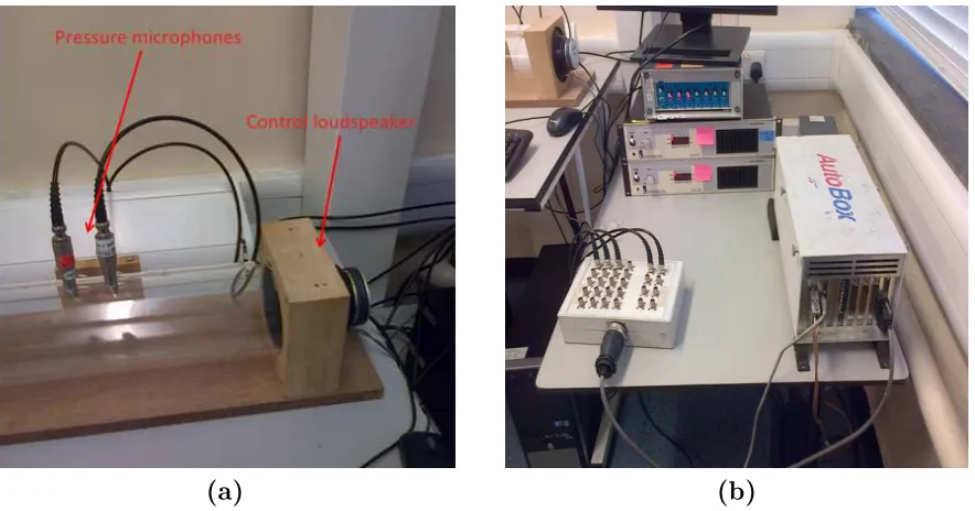
Figure 1: Picture of the experimental acoustic tube consisting of the disturbance source (near end), control source (far end) and the three sensors (two microphones and the accelerometer).

[image:8.612.199.414.371.497.2]

(9)

(a) (b)

Figure 3: (a) Control loudspeaker with embedded accelerometer and two pressure microphones. (b) dSPACE PPC Controller Board, Power Ampliers and Pre-ampliers required to implement the proposed control strategy.

III Calibration and Separation technique

[image:9.612.88.530.111.343.2]

(10)

ad-dition of this lter the microphones are now matched. When applying the lter, the signal recorded by both microphones will be nearly identical. Finally, because the driv-ing signal was random white noise (coverdriv-ing the full frequency range needed to perform experiments) the matching of the microphones is assured over this frequency range and thus control can be safely applied on the full range of frequencies.

Because the environment will always change (air temperature, humidity etc.) the calibration of the microphones should be performed every time experiments are carried out. Furthermore, small variations of the amplier gains due to temperature variations can also aect the matching.

The signal retrieved from the two microphones is the superposition of two acoustic pressure waves, the incident pi and the reecting pr. Due to wave periodicity the two

components can be separated using signals from the two microphones that are spaced with known distance ∆x1 from each other, as shown in gure 2. In the time domain,

the total pressure wave (incident and reecting) has the following mathematical form [10]:

ptot(x, t) = pi(x, t) +pr(x, t) (1)

With the illustrated experimental set-up, the microphones pick up the following pressure signals [10], respectively:

mic1 =pi(x1, t) +pr(x1, t) (2)

(11)

Where τ = ∆x1/c [s] and is the time required for the acoustic wave to travel the

predetermined distance ∆x1 between the two microphones (0.0428 [m] , gure 2) and

cis the speed of sound in air (for the experimental case studied a value of343.3[m/s] is assumed). If a time delay equal toτ is applied to the signal from microphone 2 and the signal from microphone 1 is subtracted then the following result is achieved [10]:

mic2τ =pi(x1, t) +pr(x1, t−2τ) (4)

Pref =mic2τ −mic1 =pr(x1, t) +pr(x1, t−2τ) (5)

Therefore, as required, the acoustic pressure signal derived in equation (5) contains only components of the reected wave. Due to the distance of the microphones, (g. 1), in order to successfully separate the standing wave into incident and reecting the appropriate time delay required will beτ =Δx1/c = 0.0428/343.3 = 0.000125[s] hence

a sampling rate of8kHz is required. From Shanon's criterion the un-modelled states of

Pref will be above4kHz. For sound waves with frequencies above4kHzthe wavelength

will be smaller than ∆x1 (distance of microphones). This implies that multiple waves will be present in the gap between the two microphones when considering frequencies greater than4 kHz (this is equivalent to a spatial Nyquist cut-o frequency).

IV H

2

feedback control

(12)

a Linear Fractional Transformation (LFT) expression of the mathematical model is required. The architecture utilised is illustrated in gure 4. The process is represented as a two-input and two-output system that is labelled asP and has a feedback controller

K that maps the measurable signalwloud to the manipulated variableEcon. Specically

the two inputs are the voltage of the disturbance loudspeaker Edis and the voltage

of the control loudspeaker Econ, the two outputs are the signal generated by the two

microphones when using equation (5) (Pref) which is to be minimised and wloud the

signal measured by the accelerometer embedded on the control loudspeaker's cone. The matrix representation of the open loop system is therefore:



 

Pref

wloud



 =



 

P11 P12

P21 P22



 



 

Edis

Econ





 (6)

For the implementation of the H2 design all four transfer functions Pij (i = 1,2

and j = 1,2) have to be identied. The identication procedure of the plant's transfer

functions is carried out by tting lters to experimentally retrieved data from the apparatus. Specically the tting is done based on the invfreqz(·) function found in

Matlab. This function implements Levi's complex curve tting algorithm [11].

The next step is to formulate theH2 problem, based on equation (6) with the LFT

(13)

[image:13.612.199.412.122.224.2]

Figure 4: Block diagram of LFT description

The goal is to minimise the performance measurement, which for the case considered here is the reected sound wave in the duct (Pref). In particular the controller is to

be designed to minimise theH2 norm of the closed loop transfer function between the

disturbance input (Edis) and the performance output (Pref). For reasons of consistency

with the control literature a discrete state space representation of the system is adopted. Specically, x(k)ǫRn is the state vector, d(k) is the disturbance input (disturbance

voltageEdis), z(k) is the performance or error output (reecting sound wavePref) and

y(k) is the measurement output (acceleration of loudspeaker cone wloud) [12]:

x(k+ 1) = Ax(k) +B1d(k) +B2u(k)

z(k) = C1x(k) +D11d(k) +D12u(k)

y(k) = C2x(k) +D21d(k) +D22u(k)

           (7)

The equivalent compact matrix representation is given by:

P =      

A B1 B2

C1 D11 D12

C2 D21 D22

(14)

Letz =Fl(P, K)where Fl(P, K) =P11+P12K(I−P22K)−1P21.

The design of the optimal feedback controller is based on the popular two Riccati function method [13]. In order to generate the controller the general H2 algorithm

requires the following assumptions to be valid [12]:

1. (A, B2, C2) is stabilizable and detectable.

2. D12 and D21 have full rank.

3. 

 

A−jωI B2

C1 D21





has full column rank for ω.

4. 

 

A−jωI B1

C2 D21





has full column rank for ω.

5. D11 and D22 are zero.

6. D12=

   0 I  

 and D21=

0 I

.

7. DT

12C1 = 0 and B1DT21= 0.

8. (A, B1)is stabilizable and (A, C1)is detectable.

Given the assumptions are satised, a stabilising controller Kopt(jω) exists if and only

if:

1. X1 ≥0 is a solution to the algebraic Riccati equation:

AT_X

(15)

2. Y1 ≥0is a solution to the algebraic Riccati equation:

AY1+Y1AT +B1B1T +Y1(−C1TC1)Y1 = 0

And in conclusion, the optimal controller is then given by the following formula:

Kopt(jω) =



 

ˆ

A2 −L2

F2 0





 (9)

Where _Aˆ₂ ₌_A₊_B₂_F₂ ₊_L₂_C₂_, _L₂ ₌₋_Y₁_CT

2 and F2 =−B2TX1 .

(16)

the experimental rig.

In order to evaluate the level of performance of the H2 feedback design it is

ap-propriate to compare the design with a well established control design. Therefore, the FXLMS method is chosen and implemented on the apparatus.

V FxLMS Control Design

Over the past few decades active sound control has become a realisable and ecient control concept many control algorithms have been developed. One of the most well known of which is, `Filtered- x' Least Mean Squares (FxLMS), a full account of which is located in Adaptive Signal Processing [15]. The algorithm carries out a gradient descent adaptation rule, Least Mean Square (LMS), for a ltered version of the reference signal. It is important to emphasise the use of the ltered reference signal rather than feeding the raw error signal to the adaptation rule and by doing so, possible instability is avoided.

The popularity of this algorithm centres on its ease of implementation and robust-ness, i.e. convergence can be achieved with up to900 _{phase error in the forward path}

estimate [16]. However the FxLMS algorithm is prone to long convergence times, es-pecially in random noise disturbance, due to the small value of alpha (the convergence coecient). If the alpha is increased to too high a value, instability in the system can rapidly result.

(17)

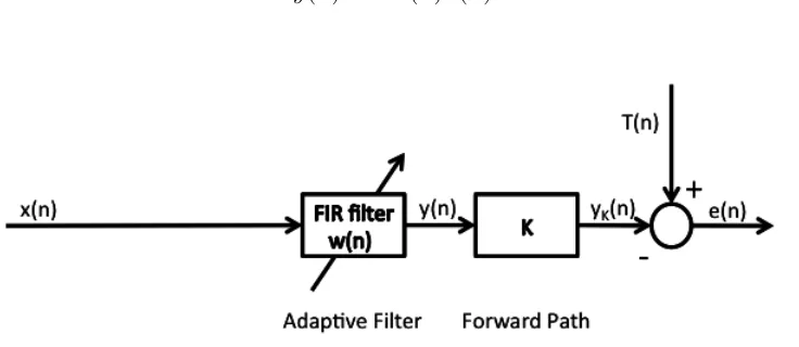
the vector inner product (for each sample instantn):

[image:17.612.125.493.174.334.2]

y(n) = wT₍_n₎_x₍_n₎ ₍₁₀₎

Figure 5: Block diagram of feedforward LMS algorithm.

Wherex(n)is the input signal vector that is fed to the adaptive lter and is expressed

as:

x(n) = [x(n), x(n−1), ..., x(n−M + 1)]T ₍₁₁₎

Furthermore w(n), is the vector of lter coecients to be found:

w(n) = [w0(n), w1(n), ..., wM−1(n)]

T ₍₁₂₎

In control applications, the estimation errore(n)is dened by the dierence between

the desired signal (desired response)d(n)and the output signal from the forward path

(18)

e(n) = d(n)−yC(n) (13)

If it is assumed that the the transfer function of the control path can be represented by anI−th order FIR lter the following mathematical description is valid:

hC(n) =

  

 

cn when nǫ{0, ..., I−1}

0 otherwise

(14)

With this the error can be represented by:

e(n) = d(n)−

I−1

X

i=0

ci M−1

X

m=0

wm(n−i)x(n−i−m) (15)

The Wiener (Mean Square Error) solution of the coecient vector is obtained by minimising the quadratic function [16, 15]:

Jf(n) =E[e2(n)] (16)

And this can be carried out by using the gradient vector for the mean square error

Jf(n):

∇w(n)Jf(n) = 2E[e(n)∇w(n)e(n)] (17)

By taking advantage of the fact that the desired signal d(n) is independent of the

(19)

∇w(n)e(n) =            −

I−1

P

i=0

cix(n−i)

−

I−1

P

i=0

cix(n−i−1)

... −

I−1

P

i=0

cix(n−i−M + 1)

           (18)

By inserting equation (18) in equation (17) we obtain the following relation for the gradient vector of the mean square error:

∇w(n)Jf(n) =−2E[e(n)xC(n)] (19)

Where xC(n) is given by the following vector:

xC(n) =

           −

I−1

P

i=0

cix(n−i)

−

I−1

P

i=0

cix(n−i−1)

... −

I−1

P

i=0

cix(n−i−M + 1)

           (20)

The LMS with a gradient estimate is then given by:

∇w(n)J ∗

f(n) = −2e(n)xC(n) (21)

(20)

LMS algorithm uses a gradient estimatex(n)e(n)which is not correct in the mean [18].

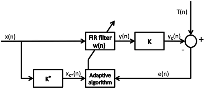
[image:20.612.139.475.229.377.2]

A compensated algorithm is obtained by ltering the reference signal to the coef-cient adjustment algorithm using a model of the forward path. The Active control system with a controller based on the FxLMS algorithm is illustrated in 6 [19].

Figure 6: Block diagram of a plant with an active controller tuned with the FxLMS algorithm

The FxLMS algorithm is given by the following equations:

y(n) = wT(n)x(n) (22)

(21)

xC∗(n) =            −

I−1

P

i=0

c∗

ix(n−i)

−

I−1

P

i=0

c∗

ix(n−i−1)

... −

I−1

P

i=0

c∗

ix(n−i−M+ 1)

           (24)

And so the update of the weights in the adaptive lter is:

w(n+ 1) =w(n) +µxC∗(n)e(n) (25)

Hereµis the convergence coecient and c∗

i are the coecients of an estimated FIR

lter model of the forward path:

hC∗(n) =      c∗

n when nǫ{0, ..., I−1}

0 otherwise

(26)

It is in practice customary to use an estimate of the impulse response for the forward path. As a result, the reference signalx∗

C(n) will be an approximation, and dierences

between the estimate of the forward path and the true forward path inuence both the stability properties and the convergence rate of the algorithm [18, 16, 17]. However, the algorithm is robust to errors in the estimate of the forward path [18, 16, 17]. The model used should introduce a time delay corresponding to the forward paths at the dominating frequencies [18, 17]. In the case of narrow-band reference signals to the algorithm the algorithm will converge with phase errors in the estimate of the forward path with up to 900_{, provided that the convergence coecient} _µ _{is suciently}

(22)

than 450 _{will have only a minor inuence on the algorithm convergence rate [20].}

In order to ensure that the action of the FxLMS algorithm is stable the maximum value for the convergence coecientµshould be given approximately by [21]:

µmax ≈

2

E[x2_C*₍_n_)](_M ₊_δ₎ (27)

whereδ is the overall delay in the forward path (in samplesn).

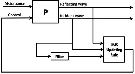
[image:22.612.191.422.326.453.2]

The block diagram utilised for the purpose of tuning the adaptive controller is viewed in gure 7.

Figure 7: Block diagram for implementing FxLMS design. P is the M IM O plant's dynamics. The block with label lter is a transfer function that replicates the path between control to reecting wave. Finally the updating rule block is formulated based on the theory developed in the previous chapter.

VI Results and analysis

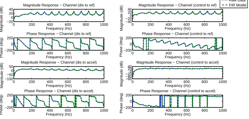
As mentioned in the previous section, models of the control and disturbance paths are required in order to derive theH2 controller. The frequency response of the high order

(23)

gure 8. In more detail, gure 8 shows the disturbance and control paths of the acoustic duct set-up previously described in equation (6).From gure 8 it is clear that the high order FIR model of the plant provides an ideal t and includes with high precision the dynamics of the pulse tube and loudspeakers. Furthermore, due to the high precision of the control path model it is possible to inspect the stability and robustness of a control design before it is applied directly on the pulse tube preventing any potential damage to the equipment. It must be emphasised that for the needs of this experiment, a random white noise signal was injected to the plant via the disturbance path (disturbance loudspeaker). The choice of white noise was done in order to guaranty the excitation of all the acoustic resonances found in the apparatus.

However as noted above, due to the high order of the model used to describe the plants dynamics, a stable and implementable feedback controller requires a reduced or-der plant with good accuracy across a smaller frequency range. The frequency response of the reduced order model is illustrated in gure 9. The reduced order model is also highly accurate across the targeted range. The sample rate of the reduced order plant has to remain at8 kHz. This is due to the distance ∆x1 between the two microphones and the separation method implemented to acquire the reecting sound wave. The predictions of the reduced order model beyond the range of interest will be poor as the dynamics of the plant are not consider during the tting procedure.

The performance of the H2 control design is demonstrated with a experimental

response of the plant, gure 10. Because the controller is designed based on a re-duced order model for a frequency band between 0-250 Hz the benecial eect of the

H2 feedback controller is most clearly observed with a signicant 10 dB reduction at

(24)

resonance within the design bandwidth the higher order modes remain unaected. De-pending on the application and disturbance source, the higher order modes could be included by systematically extending the order of the model and controller.

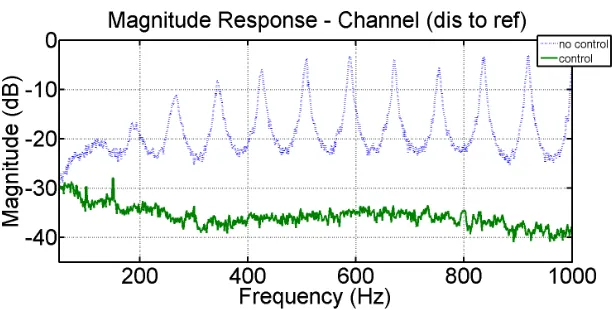
In order to evaluate the level of performance of the FxLMS controller applied on the apparatus, the magnitude of the reecting wave's power spectral density is illustrated in gure 11. By selecting an order of256for the adaptive controller, the design reduces

the reecting sound wave for a bandwidth of 100− 800 Hz. The high order of the

controller allows a signicant reduction of the reecting sound wave. Specically in gure 11, a minimum reduction of 15dB and maximum of 30dB can be viewed after the rst acoustic resonance (185Hz).

With regards to performance it can be viewed clearly that the FxLMS controller is able to reduce the undesired reecting sound wave more than the H2 local controller.

Furthermore the adaptive controller is able to apply control to a larger bandwidth compared to the H2 feedback controller. The reason the H2 controller has a smaller

(25)

a number of trial tests on the test rig it's self in order to guarantee stability had to be conducted. In terms of implementation complexity, the H2 control design is far more

superior. Specically, the FxLMS controller requires:

An up to date feedforward lter of the control path.

Experimental validation of the convergence coecient (α).

Experimental validation of the optimal order of the adaptive control.

The stability of the design can only be addressed online.

Real time measurements of the remote variables (incident and reecting sound wave).

In order to appreciate the benets when selecting the H2 design, a summary of them

is listed bellow:

To run the controller in realtime, theH2design requires for implementation only a

local signal from the accelerometer embedded on the control loudspeaker, whereas the adaptive controller requires the signal from a pair of high precision pressure microphones that results in a considerable increase of cost and implementation complexity. The H2 requires the error signal only during the control design.

The stability analysis of theH2 design is much simpler to carry out in comparison

to the FxLMS approach and can be evaluated oine.

TheH2 controller is a fully automated design and does not require any ne tuning

(26)

In conclusion, the feedback design is a much more cost and resource ecient approach in comparison to the adaptive controller. This design option is more favourable when global measurements (microphones) are not feasible for control implementation and has great potential in producing a practically viable and low cost distributed ANC system using easily accessible local measurements.

0 200 400 600 800 1000 −20 0 20 40 Frequency (Hz) Magnitude (dB)

Magnitude Response − Channel (dis to ref)

0 200 400 600 800 1000 −200

0 200

Frequency (Hz)

Phase (deg)

Phase Response − Channel (dis to ref)

0 200 400 600 800 1000 −40 −200 20 40 Frequency (Hz) Magnitude (dB)

Magnitude Response − Channel (control to ref)

0 200 400 600 800 1000 −200

0 200

Frequency (Hz)

Phase (deg)

Phase Response − Channel (control to ref)

0 200 400 600 800 1000 −100 −50 0 50 Frequency (Hz) Magnitude (dB)

Magnitude Response − Channel (dis to accel)

0 200 400 600 800 1000 −200

0 200

Frequency (Hz)

Phase (deg)

Phase Response − Channel (dis to accel)

0 200 400 600 800 1000 −60 −40 −200 20 40 Frequency (Hz) Magnitude (dB)

Magnitude Response − Channel (control to accel)

0 200 400 600 800 1000 −200

0 200

Frequency (Hz)

Phase (deg)

Phase Response − Channel (control to accel)

[image:26.612.120.528.245.440.2]

Raw Data FIR Model

(27)

0 200 400 600 800 1000 −20 0 20 40 Frequency (Hz) Magnitude (dB)

Magnitude Response − Channel (dis to ref)

0 200 400 600 800 1000

−200 0 200

Frequency (Hz)

Phase (deg)

Phase Response − Channel (dis to ref)

0 200 400 600 800 1000

−40 −20 0 20 40 Frequency (Hz) Magnitude (dB)

Magnitude Response − Channel (control to ref)

0 200 400 600 800 1000

−200 0 200

Frequency (Hz)

Phase (deg)

Phase Response − Channel (control to ref)

0 200 400 600 800 1000

−100 −50 0 50 Frequency (Hz) Magnitude (dB)

Magnitude Response − Channel (dis to accel)

0 200 400 600 800 1000

−200 0 200

Frequency (Hz)

Phase (deg)

Phase Response − Channel (dis to accel)

0 200 400 600 800 1000

−60 −40 −200 20 40 Frequency (Hz) Magnitude (dB)

Magnitude Response − Channel (control to accel)

0 200 400 600 800 1000

−200 0 200

Frequency (Hz)

Phase (deg)

Phase Response − Channel (control to accel)

[image:27.612.121.524.115.315.2]

Raw data Low order model

Figure 9: Bode plot of the raw experimental data for the disturbance and control paths (solid line) and Bode plot of the reduced order model tted to the experimental data (dashed line).

[image:27.612.156.469.409.564.2]

(28)

[image:28.612.154.460.110.265.2]

Figure 11: Magnitude of the power spectral density of the reecting sound wave without control and with FxLMS feedforward control for experimental response (dashed line, solid line)

VII Conclusions

In this paper a systematic approach to the design of an ANC system was developed in order to achieve reduction of the reected sound waves in an experimental one-dimensional acoustic duct problem. The method makes use of a robust and near-optimal H2 generalised feedback controller and has been shown experimentally to be

(29)

of the compensator together with the associated computational burden.

Acknowledgement

The author's would like to acknowledge support from EPSRC and the Onassis found-ation during the course of this work.

References

[1] S.M. Kuo and D. Morgan, Active noise control systems: algorithms and DSP im-plementations, (John Wiley & Sons, Inc. New York, NY, USA, 1995) pp. 17101.

[2] S.M. Kuo and D.R. Morgan, Active noise control: a tutorial review, Proceedings of the IEEE. 87(6), 943973(1999).

[3] X. Yu and H. Zhu and R. Rajamani and K.A. Stelson, K. A., Acoustic trans-mission control using active panels: an experimental study of its limitations and possibilities, Smart Materials and Structures. 16(6), 2006(2007).

[4] H. Zhu and R. Rajamani and K.A Stelson, Active control of acoustic reection, absorption, and transmission using thin panel speakers, The Journal of the Acous-tical Society of America. 113, 852(2003).

(30)

[6] J. S. Vipperman and R. L. Clark, Multivariable feedback active structural acoustic control using adaptive piezoelectric sensoriactuators, The Journal of the Acous-tical Society of America. 105(1), 219225(1999).

[7] M. R. Bai and H. H. Lin, Comparison of active noise control structures in the presence of acoustical feedback by using the H-innity synthesis technique, Journal of Sound and Vibration. 206(4), 453471(1997).

[8] H. Lissek and R. Boulandet and R. Fleury, R., Electroacoustic absorbers: bridging the gap between shunt loudspeakers and active sound absorption, The Journal of the Acoustical Society of America. 129, 2968(2011).

[9] ISO 10354-2: Acoustics - Determination of sound absorption coecient and im-pedance in imim-pedance tubes - Part 2: transfer-function method, (1996).

[10] D. Guicking, Recent advances in active noise control, Recent Developments in Air-and Structure-Borne Sound and Vibration. 1, 313320(1992).

[11] E. C. Levy, Complex-Curve Fitting, IRE Transactions on Automatic Control. 4, 3744(1959).

[12] S. Skogestad and I. Postlethwaite, Multivariable feedback control: analysis and design, volume 2 (Wiley, England, 1997), pp. 362365.

(31)

[14] M. Green and D.J.N. Limebeer, Linear robust control (Dover Publications, Inc., Mineola, New York, 2012), pp. 131178.

[15] B. Widrow and S.D. Stearns, Adaptive signal processing (Englewood Clis, NJ, Prentice-Hall, Inc., 1985), chapter 3.

[16] P.A. Nelson and S.J. Elliott and J.E.F Williams, Active control of sound (Academic Press Inc, London, 1993), pp. 161200.

[17] D.R. Morgan, D. R., An analysis of multiple correlation cancellation loops with a lter in the auxiliary path, Acoustics, Speech and Signal Processing, IEEE Transactions on. 28(4), 454467(1980).

[18] S.J. Elliott and I. Stothers and P.A. Nelson, A multiple error LMS algorithm and its application to the active control of sound and vibration, Acoustics, Speech and Signal Processing, IEEE Transactions on. 35(10), 14231434(1987).

[19] L. Hakansson, The ltered-X LMS algorithm, University of Karlskrona/Ronneby, 14 (2004).

[20] C.C. Boucher and S.J. Elliott and P.A. Nelson, Eect of errors in the plant model on the performance of algorithms for adaptive feedforward control, IEE Proceed-ings F (Radar and Signal Processing). 138(4), 313319 (1991).

(32)

List of gure captions

Figure1 Picture of the experimental acoustic tube consisting of the disturbance source (near end), control source (far end) and the three sensors (two mi-crophones and the accelerometer).

Figure2 Illustration of the experimental acoustic duct of length L = 2.05 [m] and diameter d = 0.099 [m]. A Disturbance source at one end of the duct (D) and control source at the other end (C). Two pressure microphones are placed near the control source at distance ∆x1 = 0.0428 [m] from each other and ∆x2 = 0.2 [m] from the control loudspeaker. Microphone 1 is at distance x1 =L−∆x1−∆x2 = 1.8112 [m] and Microphone 2 at distance x2 =x1+ ∆x1 = 1.854 [m]. The Accelerometer is connected on the cone of

the control loudspeaker (labelled with C).

Figure3 (a) Control loudspeaker with embedded accelerometer and two pressure microphones. (b) dSPACE PPC Controller Board, Power Ampliers and Pre-ampliers required to implement the proposed control strategy.

Figure4 Block diagram of LFT description.

Figure5 Block diagram of feedforward LMS algorithm.

Figure6 Block diagram of a plant with an active controller tuned with the FxLMS algorithm.

(33)

the path between control to reecting wave. Finally the updating rule block is formulated based on the theory developed in the previous chapter.

Figure8 Bode plot of the raw experimental data for the disturbance and control paths (solid line) and Bode plot of the high order FIR lter tted to the experimental data (dashed line).

Figure9 Bode plot of the raw experimental data for the disturbance and control paths (solid line) and Bode plot of the reduced order FIR lter tted to the experimental data (dashed line).

Figure10 Magnitude of the power spectral density of the reecting sound wave without and with localH2 feedback control for experimental data (dashed line, solid

line).

Figure11 Magnitude of the power spectral density of the reecting sound wave without control and with FxLMS feedforward control for experimental response (dashed line, solid line).