This is a repository copy of A quantum Jensen-Shannon graph kernel for unattributed graphs.
White Rose Research Online URL for this paper: http://eprints.whiterose.ac.uk/116511/
Version: Submitted Version
Article:
Bai, Lu, Rossi, Luca, Torsello, Andrea et al. (1 more author) (2015) A quantum
Jensen-Shannon graph kernel for unattributed graphs. Pattern Recognition. pp. 344-355. ISSN 0031-3203
https://doi.org/10.1016/j.patcog.2014.03.028
Reuse
Items deposited in White Rose Research Online are protected by copyright, with all rights reserved unless indicated otherwise. They may be downloaded and/or printed for private study, or other acts as permitted by national copyright laws. The publisher or other rights holders may allow further reproduction and re-use of the full text version. This is indicated by the licence information on the White Rose Research Online record for the item.
Takedown
If you consider content in White Rose Research Online to be in breach of UK law, please notify us by
A Quantum Jensen-Shannon Graph Kernel for Unattributed Graphs
Lu Bai1, Luca Rossi2∗, Andrea Torsello3, Edwin R. Hancock1∗∗
1
Department of Computer Science, The University of York, York YO10 5DD, UK
2
School of Computer Science, University of Birmingham, UK
3
Department of Environmental Science, Informatics, and Statistics, Ca’ Foscari University of Venice, Italy
Abstract
In this paper, we use the quantum Jensen-Shannon divergence as a means of measuring the
in-formation theoretic dissimilarity of graphs and thus develop a novel graph kernel. In quantum
mechanics, the quantum Jensen-Shannon divergence can be used to measure the dissimilarity of
quantum systems specified in terms of their density matrices. We commence by computing the
density matrix associated with a continuous-time quantum walk over each graph being compared.
In particular, we adopt the closed form solution of the density matrix introduced in [27, 28] to
re-duce the computational complexity and to avoid the cumbersome task of simulating the quantum
walk evolution explicitly. Next, we compare the mixed states represented by the density matrices
using the quantum Jensen-Shannon divergence. With the quantum states for a pair of graphs
de-scribed by their density matrices to hand, the quantum graph kernel between the pair of graphs is
defined using the quantum Jensen-Shannon divergence between the graph density matrices. We
evaluate the performance of our kernel on several standard graph datasets from both
bioinformat-ics and computer vision. The experimental results demonstrate the effectiveness of the proposed
quantum graph kernel.
Keywords: Graph Kernels, Continuous-time Quantum Walk, Quantum State, Quantum
Jensen-Shannon Divergence
∗Corresponding author. Lu Bai. Tel.: +86 13084142051 (P.R. CHINA); +44 (0)7429399030 (UK).
∗∗Corresponding author. Luca Rossi. Tel.: +44 (0) 1214144766 (UK).
Edwin R. Hancock is supported by a Royal Society Wolfson Research Merit Award.
1. Introduction
Structural representations have been used for over 30 years in pattern recognition due to their
representational power. However, the increased descriptiveness comes at the cost of a greater
dif-ficulty in applying standard techniques to them, as these usually require data to reside in a vector
space. The famous kernel trick [1] allows the focus to be shifted from the vectorial representation
of data, which now becomes implicit, to a similarity representation. This allows standard learning
techniques to be applied to data for which no obvious vectorial representation exists. For this
rea-son, in recent years pattern recognition has witnessed an increasing interest in structural learning
using graph kernels.
1.1. Literature Review
1.1.1. Graph Kernels
One of the most influential works on structural kernels was the generic R-convolution kernel
proposed by Haussler [2]. Here graph kernels are computed by comparing the similarity of each of
the decompositions of the two graphs. Depending on how the graphs are decomposed, we obtain
different kernels. Generally speaking, most R-convolution kernels count the number of
isomor-phic substructures in the two graphs. Kashima et al. [3] compute the kernel by decomposing the
graph into random walks, while Borgwardt et al. [4] have proposed a kernel based on shortest
paths. Here, the similarity is determined by counting the numbers of pairs of shortest paths of the
same length in a pair of graphs. Shervashidze et al. [5] have developed a subtree kernel on
sub-trees of limited size. They compute the number of subsub-trees shared between two graphs using the
Weisfeiler-Lehman graph invariant. Aziz et al. [6] have defined a backtrackless kernel on cycles
of limited length. They compute the kernel value by counting the numbers of pairs of cycles of
the same length in a pair of graphs. Costa and Grave [7] have defined a so-called neighborhood
subgraph pairwise distance kernel by counting the number of pairs of isomorphic neighborhood
subgraphs. Recently, Kriege et al [8] counted the number of isomorphisms between pairs of
sub-graphs, while Neumann et al. [9] have introduced the concept of propagation kernels to handle
One drawback of these kernels is that they neglect the locational information for the
substruc-tures in a graph. In other words, the similarity does not depend on the relationships between
sub-structures. As a consequence, these kernels cannot establish reliable structural correspondences
between the substructures. This limits the precision of the resulting similarity measure. To
over-come this problem, Fr¨ohlich et al. [10] introduced alternative optimal assignment kernels. Here
each pair of structures is aligned before comparison. However, the introduction of the alignment
step results in a kernel that is not positive definite in general [11]. The problem results from the
fact that alignments are not in general transitive. In other words, ifσ is the vertex-alignment be-tween graphAand graphB, andπis the alignment between graphBand graphC, in general we
cannot guarantee that the alignment between graphAand graph C is π◦σ. On the other hand, when the alignments are transitive, there is a common simultaneous alignment of all the graphs.
Under this alignment, the optimal assignment kernel is simply the sum over all the vertex/edge
kernels, and this is positive definite since it is the sum of separate positive definite kernels. While
lacking positive definiteness the optimal assignment kernels cannot be guaranteed to represent an
implicit embedding into a Hilbert space, they have nonetheless been proven to be very effective
in classifying structures. Another example of alignment-based kernels are the edit-distance-based
kernels introduced by Neuhaus and Bunke [12]. Here the alignments obtained from graph-edit
distance are used to guide random walks on the structures being compared.
An attractive alternative way to measure the similarity of a pair of graphs is to use the mutual
information and compute the classical Jensen-Shannon divergence [13]. In information theory,
the Jensen-Shannon divergence is a dissimilarity measure between probability distributions. It is
symmetric, always well defined and bounded [13]. Bai and Hancock [14] have used the
diver-gence to define a Jensen-Shannon kernel for graphs. Here, the kernel between a pair of graphs is
computed using a nonextensive entropy measure in terms of the classical Jensen-Shannon
diver-gence between probability distributions over graphs. For a graph, the elements of the probability
distribution are computed from the degree of corresponding vertices. The entropy associated with
a probability distribution of an individual graph can thus be directly computed without the need of
decomposing the graph into substructures. Hence, unlike the aforementioned existing graph
task of determining the similarities between all pairs of substructures. Unfortunately, the required
composite entropy for the Jensen-Shannon kernel is computed from a product graph formed by
a pair of graphs, and reflects no correspondence information between pairs of vertices. As a
re-sult, the Jensen-Shannon graph kernel lacks correspondence information between the probability
distributions over the graphs, and thus cannot precisely reflect the similarity between graphs.
There has recently been an increasing interest in quantum computing because of the potential
speed-ups over classical algorithms. Examples include Grover’s polynomially faster search
al-gorithm [15] and Shor’s exponentially faster factorization alal-gorithm [16]. Furthermore, quantum
algorithms also offer us a richer structure than their classical counterparts since they use qubits
rather than bits as the basic representational unit [17].
1.1.2. Quantum Computation
Quantum systems differ from their classical counterparts, since they add the possibility of
state entanglement to the classical statistical mixture of classical systems, which results in an
ex-ponential increase of the dimensionality of the state-space which is at the basis of the quantum
speedup. Pure quantum states are represented as entries in a complex Hilbert space, while
poten-tially mixed quantum states are represented through the density matrix. Mixed states can then be
compared by examining their density matrices. One convenient way to do this is to use the
quan-tum Jensen-Shannon divergence, first introduced by Majtey et al. [13, 18]. Unlike the classical
Jensen-Shannon divergence which is defined as a similarity measure between probability
distribu-tions, the quantum Jensen-Shannon divergence is defined as the distance measure between mixed
quantum states described by density matrices. Moreover, it can be used to measure both the degree
of mixing and entanglement [13, 18].
In this paper, we are interested in computing a kernel between pairs of graphs using the
quan-tum Jensen-Shannon divergence between two mixed states representing the evolution of
continuous-time quantum walks on the graphs. The continuous-continuous-time quantum walk has been introduced as the
natural quantum analogue of the classical random walk by Farhi and Gutmann in [19], and has
been widely used in the design of novel quantum algorithms. Ambainis et al. [20, 21] were among
have explored the application of quantum walks on graphs to a number of problems [22]. Childs
et al. [23, 24] have explored the difference between quantum and classical random walks, and then
exploited the increased power of quantum walk as a general model of computation.
Similar to the classical random walk on a graph, the state space of the continuous-time quantum
walk is the set of vertices of the graph. However, unlike the classical random walk where the state
vector is real-valued and the evolution is governed by a doubly stochastic matrix, the state vector
of the continuous-time quantum walk is complex-valued and its evolution is governed by a
time-varying unitary matrix. The continuous-time quantum walk possesses a number of interesting
properties which are not exhibited by the classical random walk. For instance, the
continuous-time quantum walk is reversible and non-ergodic, and does not have a limiting distribution. As a
result, the continuous-time quantum walk offers us an elegant way to design quantum algorithms
on graphs. For further details on quantum computation and quantum algorithms, we refer the
reader to the textbook in [17].
There have recently been several attempts to define quantum kernels using the
continuous-time quantum walk. For instance, Bai et al. [26] have introduced a novel graph kernel where the
similarity between two graphs is defined in terms of the similarity between two quantum walks
evolving on the two graphs. The basic idea here is to associate with each graph a mixed
quan-tum state representing the time evolution of a quanquan-tum walk. The kernel between the walk is
defined as the divergence between the corresponding density operators. However, this quantum
divergence measure requires the computation of an additional mixed state where the system has
equal probability of being in each of the two original quantum states. Unless this quantum kernel
takes into account the correspondences between the vertices of the two graphs, it can be shown
that it is not permutation invariant. Rossi et al. [27, 28] have attempted to overcome this problem
by allowing the two quantum walks to evolve on the union of the two graphs. This exploits the
relation between the intereferences of the continuous-time quantum walks and the symmetries in
the structures being compared. Since both the mixed states are defined on the same structure,
this quantum kernel addresses the shortcoming of permutation variance. However, the resulting
approach is less intuitive, thus making it particularly hard to prove the positive semidefiniteness of
two graphs, and thus also lacks vertex correspondence information. As a result, this kernel cannot
reflect precise similarity between the two graphs.
1.2. Contributions
The aim of this paper is to overcome the shortcomings of the existing graph kernels by defining
a novel quantum kernel. To this end, we develop the work in [26] further. We intend to solve the
problems of permutation variance and missing vertex correspondence by introducing an additional
alignment step, and thus compute an aligned mixed density matrix. The goal of the alignment is
to provide vertex correspondences and a lower bound on the divergence over permutations of the
vertices/quantum states. However we approximate the alignment that minimizes the divergence
with that which minimizes the Frobenious norm between the density operators. This latter
prob-lem is solved using Umeyama’s graph matching method [29]. Since the aligned density matrix is
computed by taking into account the vertex correspondences between the two graphs, the density
matrix reflects the locational correspondences between the quantum walks over the vertices of the
two graphs. As a result, our new quantum kernel can not only overcome the shortcomings of
miss-ing vertex correspondence and permutation variance that arise with the existmiss-ing kernels from the
classical/quantum Jensen-Shannon divergence, but also overcomes the shortcoming of neglecting
locational correspondence between substructures that arises in the existing R-convolution kernels.
Furthermore, in contrast to what is done in previous assignment-based kernels, we do not align the
structures directly. Rather we align the density matrices, which are a special case of a Laplacian
family signature [30] which are well known to provide a more robust representation for
correspon-dence estimation. Finally, we adopt the closed form solution of the density matrix introduced
in [27, 28] to reduce the computational complexity and to avoid the cumbersome task of explicitly
simulating the time evolution of the quantum walk. We evaluate the performance of our kernel on
several standard graph datasets from bioinformatics and computer vision. The experimental results
demonstrate the effectiveness of the proposed graph kernel, providing both a higher classification
accuracy than the unaligned kernel and also achieving a performance comparable or superior to
1.3. Paper Outline
In Section 2, we introduce the quantum mechanical formalism that will be used to develop the
ideas proposed in the paper. We describe how to compute a density matrix for the mixed quantum
state of the continuous-time quantum walk on a graph. With the mixed state density matrix to
hand, we compute the von Neumann entropy of the continuous-time quantum walk on the graph.
In Section 3, we compute a graph kernel using the quantum Jensen-Shannon divergence between
the density matrices for a pair of graphs. In Section 4, we provide some experimental evaluations,
which demonstrate experimentally the effectiveness of our quantum kernel. In Section 5, we
conclude the paper and suggest future research directions.
2. Quantum Mechanical Background
In this section, we introduce the quantum mechanical formalism to be used in this work. We
commence by reviewing the concept of a continuous-time quantum walk on a graph. We then
describe how to establish a density matrix for the mixed quantum state of the graph through a
quantum walk. With the density matrix of the mixed quantum state to hand, we show how to
compute a von Neumann entropy for a graph.
2.1. The Continuous-Time Quantum Walk
The continuous-time quantum walk is a natural quantum analogue of the classical random
walk [19, 31]. Classical random walks can be used to model a diffusion process on a graph, and
have proven to be a useful tool in the analysis of graph structure. In general, diffusion is modeled
as a Markovian process defined over the vertices of the graph, where the transitions take place on
the edges. More formally, letG= (V, E)be an undirected graph, whereV is a set ofnvertices and
E = (V ×V)is a set of edges. Thestate vectorfor the walk at timetis a probability distribution
overV, i.e., a vector⃗pt ∈Rnwhoseuth entry gives the probability that the walk is at vertexuat
timet. LetAdenote the symmetric adjacency matrix of the undirected graphGand letDbe the
diagonal degree matrix with elementsdu =∑nv=1A(u, v), wheredu is the degree of the vertexu.
Then, the continuous-time random walk onGwill evolve according to the equation
whereL=D−Ais the graph Laplacian.
As in the classical case, the continuous-time quantum walk is defined as a dynamical process
over the vertices of the graph. However, in contrast to the classical case where the state vector
is constrained to lie in a probability space, in the quantum case the state of the system is defined
through a vector of complexamplitudesover the vertex setV. The squared norm of the amplitudes
sums to unity over the vertices of the graph, with no restriction on their sign or complex phase.
This in turn allows both destructive and constructive interference to take place between the
plex amplitudes. Moreover, in the quantum case the evolution of the walk is governed by a
com-plex valued unitary matrix, whereas the dynamics of the classical random walks is governed by a
stochastic matrix. Hence the evolution of the quantum walk is reversible, which implies that
quan-tum walks are non-ergodic and do not possess a limiting distribution. As a result, the behaviour
of classical and quantum walks differs significantly. In particular, the quantum walk possesses a
number of interesting properties not exhibited in the classical case. One notable consequence of
the interference properties of quantum walks is that when a quantum walker backtracks on an edge
it does so with opposite phase. This gives rise to destructive interference and reduces the problem
of tottering. In fact the faster hitting time observed in quantum walks on the line are a consequence
of the destructive interference of backtracking paths [31].
The Dirac notation, also known asbra-ketnotation, is a standard notation used for describing
quantum states. We callpure statea quantum state that can be described using a singleketvector
|a⟩. In the context of the paper, a ket vector is a complex valued column vector of unit Euclidean
length, in a n-dimensional Hilbert space. Its conjugate transpose is a bra(row) vector, denoted
as⟨a|. As a result, the inner product between two states |a⟩and|b⟩is written ⟨a|b⟩, while their outer product is|a⟩ ⟨b|. Using the Dirac notation, we denote thebasis statecorresponding to the
walk being at vertex u ∈ V as |u⟩. In other words, |u⟩ is the vector which is equal to 1 in the position corresponding to the vertex uand is zero everywhere else. A general state of the walk
is then expressed as a complex linear combination of these orthonormal basis states, such that the
state vector of the walk at timetis defined as
|ψt⟩= ∑
u∈V
where the amplitudeαu(t) ∈Cis subject to the constraints ∑
u∈V αu(t)α∗u(t) = 1for allu ∈ V, t∈R+, whereα∗
u(t)is the complex conjugate ofαu(t).
At each instant of time, the probability of the walk being at a particular vertex of the graph
G(V, E)is given by the squared norm of the amplitude associated with |ψt⟩. More formally, let Xt be a random variable giving the location of the walk at time t. The probability of the walk
being at vertexu∈V at timetis given by
Pr(Xt =u) = αu(t)α∗u(t). (3)
More generally, a quantum walker represented by |ψt⟩ can be observed to be in any state
|ϕ⟩ ∈ Cn, and not just in the states |u⟩, u ∈ V corresponding to the graph vertices. Given
an orthonormal basis|ϕ1⟩, . . . ,|ϕn⟩ofCn, the quantum walker|ψt⟩is observed in state|ϕi⟩with
probability⟨ψi|ψi⟩. After being observed on state|ϕi⟩, the new state of the quantum walker is|ϕi⟩.
Further, given the nature of quantum observation, only orthonormal states can be distinguished by
a single observation.
In quantum mechanics, theSchr¨odinger equationis a partial differential equation that describes
how quantum systems evolve with time. In the non relativistic case it assumes the form
i~∂
∂t|ψ⟩=H |ψ⟩, (4)
where theHamiltonianoperatorHaccounts for the total energy of a system. In the case of a
par-ticle moving in an empty space with zero potential energy, this reduces to the Laplacian operator
∇2. Here, we take the Hamiltonian of the system to be the graph Laplacian matrixL. However,
any Hermitian operator encoding the structure of the graph can be chosen as an alternative.
The evolution of the walk at timetis then given by the Schr¨odinger equation
∂
∂t|ψt⟩=−iL|ψt⟩, (5)
where the Laplacian Lplays the role of the system Hamiltonian. Given an initial state |ψ0⟩, the
Schr¨odinger equation has an exponential solution which can be used to determine the state of the
walk at a time,t, giving
whereUt=e−iLtis a unitary matrix governing the evolution of the walk. To simulate the evolution
of the quantum walk, it is customary to rewrite Eq.(6) in terms of the spectral decomposition
L = ΦTΛΦ of the Laplacian matrix L, where Λ = diag(λ
1, λ2, ..., λ|V|) is a diagonal matrix
with the ordered eigenvalues as elements(λ1 < λ2 < ... < λ|V|) and Φ = (ϕ1|ϕ2|...|ϕ|V|)is a
matrix with the corresponding ordered orthonormal eigenvectors as columns. Hence, Eq.(6) can
be rewritten as
|ψt⟩= ΦTe−iΛtΦ|ψ0⟩. (7)
In this work, we letαu(0)be proportional todu and using the constraints applied to the
ampli-tude we get
αu(0) = du √∑
d2 u
. (8)
Note that there is no particular indication as how to choose the initial state. However, choosing a
uniform distribution over the vertices ofGwould result in the system remaining stationary, since the initial state vector would be an eigenvector of the Laplacian ofGand thus a stationary state of
the walk.
2.2. A Density Matrix from the Mixed State
While a pure state can be naturally described using a single ket vector, in general a quantum
system can be in amixed state, i.e., a statistical ensemble of pure quantum states|ψi⟩, each with
probabilitypi. Thedensity operator(ordensity matrix) of such a system is defined as
ρ=∑
i
pi|ψi⟩ ⟨ψi|. (9)
Density operators are positive unit-trace matrices directly linked with the observables of the
(mixed) quantum system. LetObe an observable, i.e., an Hermitian operator acting on the quan-tum states and providing a measurement. Without loss of generality we have O = ∑m
i=1viPi,
where Pi is the orthogonal projector onto the i-th observation basis, and vi is the measurement
value when the quantum state is observed to be in this observation basis.
The expectation value of the measurement over a mixed state can be calculated from the density
matrixρ:
wheretris the trace operator. Similarly, the observation probability on thei-th observation basis
can be expressed in terms of the density matrixρas
Pr(X =i) = tr(ρPi). (11)
Finally, after the measurement, the corresponding density operator will be
ρ′ =
m ∑
i=1
PiρPi. (12)
For a graph G(V, E), let |ψt⟩ denote the state corresponding to a continuous-time quantum
walk that has evolved from timet= 0to timet =T. We define the time-averaged density matrix
ρT
GforG(V, E)
ρTG=
1 T
∫ T
0
|ψt⟩ ⟨ψt|dt, (13)
which can be expressed in terms of the initial state|ψ0⟩as
ρT G = 1 T ∫ T 0
e−iLt|ψ
0⟩ ⟨ψ0|eiLtdt. (14)
In other words,ρT
Gdescribes a system which has an equal probability of being in any of the pure
states defined by the evolution of the quantum walk from t = 0 to t = T. Using the spectral
decomposition of the Laplacian we can rewrite the previous equation as
ρTG=
1 T
∫ T
0
ΦTe−iΛtΦ|ψ0⟩ ⟨ψ0|ΦTeiΛtΦ dt. (15)
Letϕxydenote the(xy)th element of the matrix of eigenvectorsΦof the Laplacian. The(r, c)th
element ofρT can be computed as
ρT
G(r, c) =
1 T ∫ T 0 ( n ∑ k=1 n ∑ l=1
ϕrke−iλktϕlkψ0l ) ( n
∑
x=1 n ∑
y=1
ψ0xϕxyeiλytϕcy )
dt. (16)
Letψ¯k= ∑
lϕlkψ0landψ¯y = ∑
xϕxyψ0y, whereψ0ldenotes thelth element of|ψ0⟩. Then
ρTG(r, c) =
1 T ∫ T 0 ( n ∑ k=1
ϕrke−iλktψ¯k n ∑
y=1
ϕcyeiλytψ¯y )
which can be rewritten as
ρTG(r, c) = n ∑
k=1 n ∑
y=1
ϕrkϕcyψ¯kψ¯y
1 T
∫ T
0
ei(λy−λk)tdt. (18)
If we letT → ∞, Eq.(18) further simplifies to
ρ∞
G(r, c) = ∑
λ∈Λ˜ ∑
x∈Bλ ∑
yBλ
ϕrxϕcyψ¯xψ¯y, (19)
where Λ˜ is the set of distinct eigenvalues of the Laplacian matrix L and Bλ is a basis of the
eigenspace associated with λ. As a consequence, computing the time-averaged density matrix
relies on computing the eigendecomposition ofG(V, E), and hence has time complexityO(|V|3). Note that in the remainder of this paper we will simplify our notation by referring to the
time-averaged density matrix as the density matrix associated with a graph. Moreover, we will assume
thatρT
Gis computed forT → ∞, unless otherwise stated, and we will denote it asρG.
2.3. The von Neumann Entropy of a Graph
In quantum mechanics, thevon Neumann entropy[32]HN of a mixture is defined in terms of
the trace and logarithm of the density operatorρ
HN =−tr(ρlogρ) =− ∑
i
ξilnξi, (20)
whereξ1, . . . , ξnare the eigenvalues ofρ. Note that if the quantum system is a pure state|ψi⟩with
probabilitypi = 1, then the Von Neumann entropyHN(ρ) =−tr(ρlogρ)is zero. On other hand,
a mixed state generally has a non-zero Von Neumann entropy associated with its density operator.
Here we propose to associate to each graph the von Neumann entropy of the density matrix
computed as in Eq.(19). Consider a graphG(V, E), its von Neumann entropy is
HN(ρG) = −tr(ρGlogρG) = −
|V|
∑
j
λGj logλ G
j , (21)
whereλG
2.4. Quantum Jensen-Shannon Divergence
The classical Jensen-Shannon divergence is a non-extensive mutual information measure
de-fined between probability distributions over potentially structured data. It is related to the
Shan-non entropy of the two distributions [33]. Consider two (discrete) probability distributions P =
(p1, . . . , pa, . . . , pA)andQ = (q1, . . . , qb, . . . , qB), then the classical Jensen-Shannon divergence
betweenP andQis defined as
DJ S(P,Q) =HS
(P +Q
2
)
− 1
2HS(P)− 1
2HS(Q), (22)
whereHS(P) = ∑Aa=1palogpa is the Shannon entropy of distribution P. The classical
Jensen-Shannon divergence is always well defined, symmetric, negative definite and bounded, i.e.,0 ≤
DJ S ≤1.
The quantum Jensen-Shannon divergence has recently been developed as a generalization of
the classical Jensen-Shannon divergence to quantum states by Lamberti et al. [13]. Given two
density operatorsρandσ, the quantum Jensen-Shannon divergence between them is defined as
DQJ S(ρ, σ) =HN
(ρ+σ
2
)
− 1
2HN(ρ)− 1
2HN(σ). (23)
The quantum Jensen-Shannon divergence is always well defined, symmetric, negative definite and
bounded, i.e.,0≤DQJ S ≤1[13].
Additionally, the quantum Jensen-Shannon divergence verifies a number of properties which
are required for a good distinguishability measure between quantum states [13, 18]. This is a
prob-lem of key importance in quantum computation, and it requires the definition of a suitable distance
measure. Wootters [34] was the first to introduce the concept of statistical distance between pure
quantum states. His work is based on extending a distance over the space of probability
distribu-tions to the Hilbert space of pure quantum states. Similarly, the relative entropy [35] can be seen as
a generalization of the information theoretic Kullback-Leibler divergence. However, the relative
entropy is unbounded, it is not symmetric and it does not satisfy the triangle inequality.
The square root of the QJSD, on the other hand, is bounded, it is a distance and, as proved by
Lamberti et. al [13], it satisfies the triangle inequality. This is formally proved for pure states, while
the literature, most notably the Bures distance [36]. Both the Bures distance and the QJSD require
the full density matrices to be computed. However, the QJSD turns out to be faster to compute.
On the one hand, the Bures distance involves taking the square root of matrices, usually computed
through matrix diagonalization and which has time complexityO(n3), wheren is the number of
vertices in the graph. On the other hand, the QJSD simply requires computing the eigenvalues of
the density matrices, which can be done inO(n2).
3. A Quantum Jensen-Shannon Graph Kernel
In this section, we propose a novel graph kernel based on the quantum Jensen-Shannon
di-vergence between continuous-time quantum walks on different graphs. Suppose the graphs under
consideration are represented by a set{G,. . . , Ga, . . . , Gb, . . . , GN}, we consider the
continuous-time quantum walks on a pair of graphs Ga(Va, Ea) and Gb(Vb, Eb), whose mixed state density
matricesρaandρbcan be computed using Eq.(18) or Eq.(19). With the density matricesρaandρb
to hand we compute the quantum Jensen-Shannon divergenceDQJ S(ρa, ρb)using Eq.(23).
How-ever the result depends on the relative order of the vertices in the two graphs, and we need a way to
describe the mixed quantum state given by the walk on both graphs. To this end, we consider two
strategies. We refer to these as theunaligneddensity matrix and thealigneddensity matrix. In the
first case the density matrices are added maintaining the vertex order of the data. This results in
theunalignedkernel
kQJ SU(Ga, Gb) =exp(−µDQJ S(ρa, ρb)), (24)
whereµis a decay factor in the interval0< µ≤1,
DQJ S(ρa, ρb) =HN
(ρa+ρb
2
)
− 1
2HN(ρa)− 1
2HN(ρb), (25)
is the quantum Jensen Shannon divergence between the mixed state density matricesρaandρb of GaandGb, andHN(.)is the von Neumann entropy of a graph density matrix defined in Eq.(21).
Hereµ is used to ensure that the large value does not tend to dominant the kernel value, and in this work we useµ = 1. The proposed kernel can be viewed as a similarity measure between the
ignores the vertex correspondence information for a pair of graphs, it is not permutation invariant
to vertex order. Instead it relies only on the global properties and long-range interactions between
vertices to differentiate between structures.
In the second case the mixing is performed after the density matrices are optimally aligned,
thus computing a lower bound of the divergence over the setΣof state permutations. This results
in thealignedkernel
kQJ SA(Ga, Gb) = max
Q∈Σexp(−µDQJ S(ρa, QρbQ
T)) = exp(−µmin
Q∈ΣDQJ S(ρa, QρbQ
T)). (26)
Here the alignment step adds correspondence information allowing for a more fine-grained
dis-crimination between structures.
In both cases the density matrix of smaller size is padded to size of the larger one before
com-puting the divergence. Note that this is equivalent to padding the adjacency matrix of the smaller
graph to be the same size as the larger one, since both these operations are simply increasing the
dimension of the kernel of the density matrix.
3.1. Alignment of the Density Matrix
The definition of the aligned kernel requires the computation of the permutation that minimizes
the divergence between the graphs. This is equivalent to minimizing the Von Neumann entropy
of the mixed state(ρa+ρb)/2. However, this is a computationally hard task, and so we perform
a two step approximation to the problem. First, we approximate the solution by minimizing the
Frobenious (L2) distance between matrices rather than the Von Neumann entropy. Second we find
an approximate solution to theL2 problem using Umeyama’s method [29].
The rationale behind this approximate method is given by the fact that we already have the
eigenvectors and eigenvalues of the Hamiltonian to hand, and with these we can efficiently
Umeyama’s spectral approach). More precisely, the authors of [37] show that
Lρa=
∑
λ∈Λ˜
λPλPλT
∑
λ∈Λ˜
Pλρ0PλT
= ∑
λ∈Λ˜
Pλλρ0PλT =
=
∑
λ∈Λ˜
Pλρ0PλT
∑
λ∈Λ˜
λPλPλT
=ρaL, (27)
whereρ0denotes the density matrix forGat timet= 0andPλ = ∑µ(λ)
k=1 ϕλ,kϕTλ,kis the projection
operator onto the subspace spanned by theµ(λ)eigenvectorsϕλ,k associated with the eigenvalue λ of the Hamiltonian. In other words, given the spectral decomposition of the Laplacian matrix
L= ΦΛΦT, if we express the density matrix in the eigenvector basis given byΦ, then it assumes
a block diagonal form, where each block corresponds to an eigenspace ofL corresponding to a
single eigenvalue. As a consequence, ifLhas all eigenvalues distinct, thenρawill have the same
spectrum as L. Otherwise, we need to independently compute the eigendecomposition of each
diagonal block, resulting in a complexityO( ∑
λ∈Λ˜ µ(λ)2 )
, where µ(λ)denotes the multiplicity of the eigenvalueλ.
3.2. Properties of the Quantum Jensen-Shannon Kernel for Graphs
Theorem 3.1.If the Quantum Jensen-Shannon divergence is negative definite, then the unaligned
Quantum Jensen-Shannon Kernel is positive definite.
Proof. Fist note that for the computation of Quantum Jensen-Shannon divergence, padding the
smaller matrix to the size of the larger one is equivalent to padding both to an even larger size.
Thus we can consider the computation of the kernel matrix overN graphs to be performed over density matrices padded to the size of the larger graph. This eliminates the dependence of the
density matrix of the first graph on the choice of the second graph.
In [38] the authors show that ifs(Ga, Gb)is a conditionally positive semidefinite kernel, i.e.,
−s(Ga, Gb)is a negative definite kernel, thenks = exp(λs(Ga, Gb))is positive semidefinite for
anyλ >0.
Hence, if the Quantum Jensen-Shannon divergence DQJ S(Ga, Gb) is negative definite, then
−DQJ S(Ga, Gb)is conditionally positive semidefinite, and the Quantum Jensen-Shannon kernel
Note that this proof is conditioned on the negative definiteness of the Quantum Jensen-Shannon
divergence, as is the case for the classical Jensen-Shannon divergence. Currently this is only a
conjecture, proved to be true on pure quantum states, and for which there is a strong empirical
evidence [39].
In general for the optimal alignment kernel [10, 11] we cannot guarantee positive definiteness
for the aligned version of our quantum kernel due to the lack of transitivity of the alignments. We
do have, however, a similar result when using any (possibly non optimal) set of alignments that
satisfy transitivity.
Corollary 3.2. If the Quantum Jensen-Shannon divergence is negative definite and the density
matrices are aligned by a transitive set of permutations, then the unaligned Quantum
Jensen-Shannon Kernel is positive definite.
Proof. If the alignments are transitive, each of the density matrices can be aligned to a single
common frame, for example that of the first graph. The aligned kernel on the original unaligned
data is equivalent to the unaligned kernel on the new pre-aligned data.
Another important property for a kernel is its independence on the ordering of the data. There
are two ways by which the kernel can depend on this ordering: First, it might depend on the order
in which different graphs are presented. Second, it might depend on the order in which the vertices
are presented in each graph.
Since the kernel only depends on second order relations, a sufficient condition for the first
type of independence is for the kernel to be deterministic and symmetric. If this is so, then a
permutation of the graphs will just result in the same permutation to be applied to the rows and
columns of the kernel matrix. For the second type of invariance, we need full invariance of the
computed kernel values with respect to vertex permutations.
The unaligned kernel trivially satisfies the first condition since the Quantum Jensen-Shannon
divergence is both deterministic and symmetric, while it fails to satisfy the second condition, thus
resulting in a kernel that is independent on the order of the graphs, but not on the vertex order
within each graph. For the aligned kernel, on the other hand, the addition of the alignment step
requires a little more analysis.
vertex order.
Proof. Recall that given two graphsGa andGb with mixed state density matricesρa andρb, the
aligned kernel is
kQJ SA(Ga, Gb) = max
Q∈Σ exp(−µDQJ S(ρa, QρbQ T
)). (28)
As a result the kernel value is uniquely identified even when there are multiple possible alignments.
Due to their optimality these alignments must all result in the same optimal divergence. It is easy
to see that the kernel is also symmetric. In fact, since the Von Neumann entropy is invariant to
similarity transformations, we have
HN (
ρa+QρbQT
2
)
=HN (
QQ Tρ
aQ+ρb
2 Q
T )
=HN (
QTρ
aQ+ρb
2
)
. (29)
From the aboveDQJ S(ρa, QρbQT) =DQJ S(QTρaQ, ρb) = DQJ S(ρb, QTρaQ). Hence,
kQJ SA(Ga, Gb) = max
Q∈Σ exp(−µDQJ S(ρa, QρbQ
T)) (30)
= max
Q∈Σ exp(−µDQJ S(ρb, QρaQ
T)) =k
QJ SA(Gb, Ga).
As a result, the aligned kernel is deterministic and symmetric, even if the optimizer might not be.
Thus the kernel is independent of the order of the graphs.
The independence of vertex ordering again derives directly from the optimality of the value
of the divergence. LetG′b be a vertex-permuted version of Gb, such that its mixing matrixρ′b = T ρbTT for a permutation matrix T ∈ Σ, and assume that kQJ SA(Ga, G′b) ̸= kQJ SA(Ga, Gb).
Without loss of generality we can assumekQJ SA(Ga, G′b)> kQJ SA(Ga, Gb). Let
Q∗= argmax
QΣ
exp(−µDQJ S(ρa, Qρ′bQ
T)), (31)
then
exp(−µDQJ S(ρa, Q∗ρ′bQ∗ T
)) = exp(−µDQJ S(ρa, Q∗T ρbTTQ∗T)) (32)
> max
Q∈Σexp(−µDQJ S(ρa, QρbQ T
)),
leading to a contradiction.
Note that these properties depend on the optimality of the alignment with respect to the
the Frobenious (L2) norm between the density matrices. This is approximated using Umeyama’s
algorithm since the resulting matching problem is still in general NP-hard. However, in the proof
the optimality was used as a means to uniquely identify the value of the divergence. Any other
uniquely identified value would still give an order invariant kernel, even if this is suboptimal.
Eq.(3.2) does not depend on the choice of optimal alignment, and so it would still hold underL2
optimality. The main problem is whether two permutations leading to the same (minimal)
Frobe-nious distance between the density matrices can give different divergence values. If permutations
Q1 andQ2 differ by the combination of symmetries present in the two graphs, i.e., Q1 = SQ2R
with S ∈ Aut(Ga) and R ∈ Aut(Gb), then clearly they will have the same divergence since ρa = SρsST andρb = RρbRT, but that might not characterize all theL2 optimal permutations.
Nonetheless, we have the following
Theorem 3.4. If theL2 optimal permutation is unique modulo isomorphism in the two graphs,
then theL2 approximation is independent of the order of the graphs.
Proof.Derives directly from the uniqueness of the kernel value for all the optimizers.
There remains another source of error, since Umeyama’s algorithm is only an approximation to
the Frobenious minimizer. The impact of this is much wider since the lack of optimality implies an
inability to uniquely identify the value of the kernel in an invariant way. However, this is implicit
in all alignment-based approaches due to the NP hard nature of the graph matching problem.
3.3. Complexity Analysis
For a graph dataset havingN graphs, the kernel matrix of the quantum Jensen-Shannon graph
kernel can be computed using Algorithm 1.
For N graphs each of which has n vertices, the time complexity of the quantum
Jensen-Shannon graph kernel on all pairs of these graphs is given by the three computational steps of
Algorithm 1. These are: a) The computation of the density matrix for each graph. Based on the
definition in Section 2.2, this step has time complexityO(N n3). b) The computation of the aligned
density matrix and the unaligned density matrix for all pairs of graphs. This has time
complex-ities O(N2n4) and O(N2n), respectively. c) As a result, the time complexities of the quantum
Algorithm 1 Computing the kernel matrix of the quantum Jensen-Shannon graph kernel on N
graphs
Input: A graph dataset G = {G1,· · · , Ga,· · · , Gb,· · · , GN} with N test graphs. Output: A
|N| × |N|kernel matrixKQJ S.
1. Computing the density matrices of graphs: For each graphGa(Va, Ea), compute the density
matrix evolving from time0to timeT using the definition in Section 19
2. Computing the density matrix for each pair of graphs: For each pair of graphs Ga(Va, Ea)
andGb(Vb, Eb)with their density matricesρaandρb, compute ρa+2ρb using the unaligned or
the aligned procedure.
3. Computing the kernel matrix for the N graphs: Compute the kernel matrix KQJ S. For
each pair of graphsGa(Va, Ea)andGb(Vb, Eb), compute the(Ga, Gb)th element ofKQJ Sas kQJ S(Ga, Gb)using Eq.(24) or Eq.(26).
respectively.
4. Experimental Evaluation
In this section, we test our graph kernels on several standard graph based datasets. There are
three stages to our experimental evaluation. First, we evaluate the stability of the von Neumann
entropies obtained from the density matrices with timet. Second, we empirically compare our new kernel with several alternative state of the art graph kernels. Finally, we evaluate the computational
efficiency of our new kernel.
4.1. Graph Datasets
We show the performance of our quantum Jensen-Shannon graph kernel on five standard graph
based datasets from bioinformatics and computer vision. These datasets include: MUTAG, PPIs,
PTC(MR), COIL5 and Shock.
MUTAG: The MUTAG dataset consists of graphs representing 188 chemical compounds, and
aims to predict whether each compound possesses mutagenicity [40]. Since the vertices and edges
of each compound are labeled with a real number, we transform these graphs into unweighted
graphs.
PPIs: The PPIs dataset consists of protein-protein interaction networks (PPIs) [41]. The graphs
describe the interaction relationships between histidine kinase in different species of bacteria.
Histidine kinase is a key protein in the development of signal transduction. If two proteins have
direct (physical) or indirect (functional) association, they are connected by an edge. There are 219
PPIs in this dataset and they are collected from 5 different kinds of bacteria with the following
evolution order (from older to more recent)Aquifex4 andthermotoga4 PPIs fromAquifex aelicus
andThermotoga maritima,Gram-Positive52 PPIs fromStaphylococcus aureus, Cyanobacteria73
PPIs from Anabaena variabilis and Proteobacteria40 PPIs from Acidovorax avenae. There is
an additional class (Acidobacteria46 PPIs) which is more controversial in terms of the bacterial
evolution since they were discovered. Here we select Proteobacteria40 PPIs and Acidobacteria46
PPIs as the testing graphs.
PTC:The PTC (The Predictive Toxicology Challenge) dataset records the carcinogenicity of
sev-eral hundred chemical compounds for male rats (MR), female rats (FR), male mice (MM) and
female mice (FM) [42]. These graphs are very small (i.e., 20− 30 vertices), and sparse (i.e.,
25−40edges. We select the graphs of male rats (MR) for evaluation. There are344test graphs
in the MR class.
COIL5: We create a dataset referred to as COIL5 from the COIL image database. The COIL
database consists of images of 100 3D objects. In our experiments, we use the images for the first
five objects. For each of these objects we employ 72 images captured from different viewpoints.
For each image we first extract corner points using the Harris detector, and then establish Delaunay
graphs based on the corner points as vertices. Each vertex is used as the seed of a Voronoi region,
which expands radially with a constant speed. The linear collision fronts of the regions delineate
the image plane into polygons, and the Delaunay graph is the region adjacency graph for the
Voronoi polygons. Associated with each object, there are 72 graphs from the 72 different object
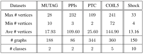
Table 1: Information of the Graph based Datasets.
Datasets MUTAG PPIs PTC COIL5 Shock
Max # vertices 28 232 109 241 33
Min # vertices 10 3 2 72 4
Ave # vertices 17.93 109.60 25.60 144.90 13.16
# graphs 188 86 344 360 150
# classes 2 2 2 5 10
hard for graph classification.
Shock: The Shock dataset consists of graphs from the Shock 2D shape database. Each graph is a
skeletal-based representation of the differential structure of the boundary of a 2D shape. There are
150 graphs divided into 10 classes. Each class contains 15 graphs.
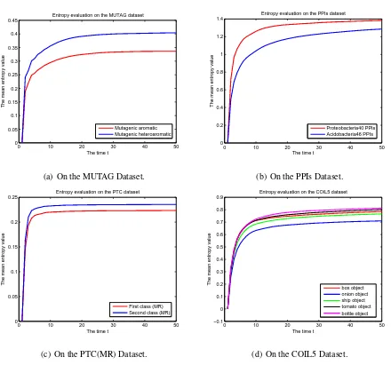
4.2. Evaluations on the von Neumann entropy with Timet
We commence by investigating the von Neumann entropy associated with the graphs as the
timetvaries. In this experiment, we use the testing graphs in the MUTAG, PPIs, PTC and COIL5 datasets, while we do not perform the evaluation on the Shock dataset. For each graph, we allow a
continuous-time quantum walk to evolve witht = 0,1,2, . . . ,50. As the walk evolves from time
t = 0 to timet = 50we compute the corresponding density matrix using Eq.(15). Thus, at each
timetwe can compute the von Neumann entropy of the corresponding density matrix associated with each graph. The experimental results are shown in Fig.1. The subfigures of Fig.1 show
the mean von Neumann entropies for the graphs in the MUTAG, PPIs, PTC and COIL5 datasets
separately. The x-axis shows the timetfrom0to50, and the y-axis shows the mean value of the
von Neumann entropies for graphs belonging to the same class. Here the different lines represent
the entropies for the different classes of graphs. These plots demonstrate that the von Neumann
0 10 20 30 40 50 0 0.05 0.1 0.15 0.2 0.25 0.3 0.35 0.4 0.45
The time t
The mean entropy value
Entropy evaluation on the MUTAG dataset
Mutagenic aromatic Mutagenic heteroaromatic
(a) On the MUTAG Dataset.
0 10 20 30 40 50 0 0.2 0.4 0.6 0.8 1 1.2 1.4
The time t
The mean entropy value
Entropy evaluation on the PPIs dataset
Proteobacteria40 PPIs Acidobacteria46 PPIs
(b) On the PPIs Dataset.
0 10 20 30 40 50 0 0.05 0.1 0.15 0.2 0.25
The mean entropy value
The time t
Entropy evaluation on the PTC dataset
First class (MR) Second class (MR)
(c) On the PTC(MR) Dataset.
0 10 20 30 40 50 −0.1 0 0.1 0.2 0.3 0.4 0.5 0.6 0.7 0.8 0.9
The time t
The mean entropy value
Entropy evaluation on the COIL5 dataset
box object onion object ship object tomato object bottle object
[image:24.595.76.516.202.613.2](d) On the COIL5 Dataset.
4.3. Experiments on Standard Graph Datasets from Bioinformatics
4.3.1. Experimental Setup
We now evaluate the performance of our quantum Jensen-Shannon kernel using both the
aligned density matrix (QJSA) and the unaligned density matrix (QJSU). Furthermore, we
com-pare our kernel with several alternative state of the art graph kernels. These kernels include 1)
the Weisfeiler-Lehman subtree kernel (WL) [5], 2) the shortest path graph kernel (SPGK) [4], 3)
the Jensen-Shannon graph kernel associated with the steady state random walk (JSGK) [14], 4)
the backtrackless random walk kernel using the Ihara zeta function based cycles (BRWK) [6], and
5) the random-walk graph kernel [3]. For our quantum kernel, we decide to lett → ∞. For the
Weisfeiler-Lehman subtree kernel, we set the dimension of the Weisfeiler-Lehman isomorphism
as10. Based on the definition in [5], this means that we compute10different Weisfeiler-Lehman
subtree kernel matrices (i.e.,k(1), k(2), . . . , k(10)) with different subtree heights h (h=1,2,. . . ,10), respectively. Note that, the WL and SPGK kernels are able to accommodate attributed graphs. In
our experiments, we use the vertex degree as a vertex label for the WL and SPGK kernels.
For each kernel and dataset, we perform a 10-fold cross-validation using a C-Support Vector
Machine (C-SVM) in order to evaluate the classification accuracies of the different kernels. More
specifically, we use the C-SVM implementation of LIBSVM [43]. For each class, we use 90% of
the samples for training and the remaining 10% for testing. The parameters of the C-SVMs are
optimized separately for each dataset. We repeat the evaluation 10 times and we report the average
classification accuracies (±standard error) of each kernel in Table 2. Furthermore, we also report
the runtime of computing the kernel matrices of each kernel in Table 3, with the runtime measured
under Matlab R2011a running on a2.5GHz Intel2-Core processor (i.e., i5-3210m). Note that, for the WL kernel the classification accuracies are the average accuracies over all the10matrices, and
the runtime refers to that required for computing all the10matrices (see [5] for details).
4.3.2. Results and Discussion
a) On the MUTAG dataset, the accuracies for all of the kernels are similar. The SPGK kernel
achieves the highest accuracy. Yet, the accuracies of our QJSA and QJSU quantum kernels are
dataset, the WL kernel achieves the highest accuracy. The accuracies of our QJSA and QJSU
quantum kernels are lower than that of the WL kernel, but outperform those of other kernels.
c) On the PTC dataset, the accuracies for all of the kernels are similar. Our QJSA quantum
kernel achieves the highest accuracy. The accuracy of our QJSU quantum kernel is competitive
or outperforms that of other kernels. d) On the COIL5 dataset, the accuracies of all the kernels
are similar with the exception of the WL, RWGK and BRWK kernels. Our QJSA quantum kernel
achieves the highest accuracy. The accuracy of our QJSU quantum kernel overcomes that of other
kernels. e) On the Shock dataset, our QJSA quantum kernel achieves the highest accuracy. The
accuracy of our QJSU quantum kernel overcomes that of other kernels.
Overall, in terms of classification accuracy our QJSA and QJSU quantum Jensen-Shannon
graph kernels outperform or are competitive with the state of the art kernels. Especially, the
clas-sification accuracies of our quantum kernel are significantly better than those of the graph kernels
using the classical Jensen-Shannon divergence, the classical random walk and the backtrackless
random walk. This suggests that our kernel, which makes use of continuous-time quantum walks
to probe the graphs structure, is successful in capturing the structural similarities between
differ-ent graphs. Furthermore, we observe that the performance of our QJSA quantum kernel is better
than that of our QJSU quantum kernel. The reason for this is that the aligned density matrix
computed through the Umeyama’s matching method can reflect the precise correspondence
infor-mation between pairs of vertices in these graphs, while the unaligned density matrix ignores the
correspondence information, and it is not permutation invariant to the vertex order.
In terms of the runtime, all the kernels can complete the computation in polynomial time on
all the datasets. The computation efficiency of our QJSU is lower than that of the WL, SPGK and
JSGK kernels, but it is faster than that of the BRWK and RWGK kernels (i.e., the kernels using
the classical random walk and the backtrackless random walk). The computational efficiency of
our QJSA kernel is lower than any alternative kernel. The reason for this is that the QJSA kernel
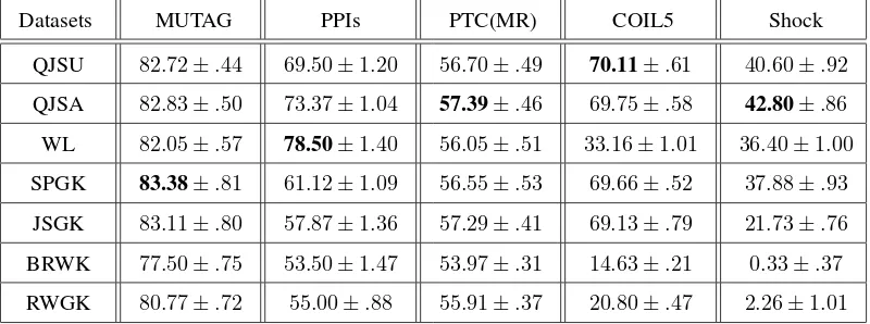
Table 2: Accuracy Comparisons (In% ±Standard Errors) on Graph Datasets abstracted from Bioinformatics and
Computer Vision.
Datasets MUTAG PPIs PTC(MR) COIL5 Shock
QJSU 82.72±.44 69.50±1.20 56.70±.49 70.11±.61 40.60±.92
QJSA 82.83±.50 73.37±1.04 57.39±.46 69.75±.58 42.80±.86
WL 82.05±.57 78.50±1.40 56.05±.51 33.16±1.01 36.40±1.00
SPGK 83.38±.81 61.12±1.09 56.55±.53 69.66±.52 37.88±.93
JSGK 83.11±.80 57.87±1.36 57.29±.41 69.13±.79 21.73±.76
BRWK 77.50±.75 53.50±1.47 53.97±.31 14.63±.21 0.33±.37
RWGK 80.77±.72 55.00±.88 55.91±.37 20.80±.47 2.26±1.01
Table 3: Runtime Comparisons on Graph Datasets abstracted from Bioinformatics and Computer Vision.
Datasets MUTAG PPIs PTC COIL5 Shock
QJSU 20” 59” 1′46” 18′20” 14”
QJSA 1′30” 23′25” 16′40” 8h29′ 32”
WL 4” 13” 11” 1′5” 3”
SPGK 1” 7” 1” 31” 1”
JSGK 1” 1” 1” 1” 1”
BRWK 2” 14′20” 3” 16′46” 8”
RWGK 46” 1′7” 2′35” 19′40” 23”
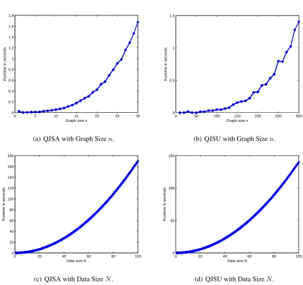
4.4. Computational Evaluation
In this subsection, we evaluate the relationship between the computational overheads (i.e., the
CPU runtime) of our kernel and the structural complexity or the number of the associated graphs.
4.4.1. Experimental setup
We evaluate the computational efficiency of our quantum kernel on randomly generated graphs
with respect to two parameters: a) the graph size n, and b) the graph dataset size N. More
specifically, we varyn={10,20, . . . ,300}andN ={1,2, . . . ,100}, separately.
We first generate 30 pairs of graphs with an increasing number of vertices. We report the
[image:27.595.152.442.349.502.2]0 5 10 15 20 25 30 0
0.2 0.4 0.6 0.8 1 1.2 1.4 1.6 1.8
Graph size n
Runtime in seconds
(a) QJSA with Graph Sizen.
0 50 100 150 200 250 300 0
0.5 1 1.5
Graph size n
Runtime in seconds
(b) QJSU with Graph Sizen.
0 20 40 60 80 100 0
20 40 60 80 100 120 140 160 180
Data size N
Runtime in seconds
(c) QJSA with Data SizeN.
0 20 40 60 80 100 0
50 100 150
Data size N
Runtime in seconds
[image:28.595.76.512.102.511.2](d) QJSU with Data SizeN.
Figure 2: Runtime Evaluation.
datasets with an increasing number of test graphs. Each test graph has50vertices. We report the
runtime for computing the kernel matrices of the graphs from each dataset. The CPU runtime is
reported in Fig.2. The experiments are run in Matlab R2011a on a 2.5GHz Intel 2-Core processor
(i.e., i5-3210m).
4.4.2. Experimental results
Fig. 2 (a) and (c) show the results obtained with the QJSA kernel, when varying the parameters
nandN, respectively. Fig. 2 (b) and (d) show those obtained with the QJSU kernel. Furthermore,
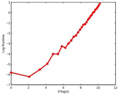
0 2 4 6 8 10 12 −6
−5 −4 −3 −2 −1 0 1
3*log(n)
Log Runtime
(a) Log Runtime vs3 log(n)using QJSA Kernel.
0 2 4 6 8 10 12 −7
−6 −5 −4 −3 −2 −1 0 1
3*log(n)
Log Runtime
(b) Log Runtime vs3 log(n)using QJSU Kernel.
0 2 4 6 8 10
−6 −4 −2 0 2 4 6
2*log(N)
Log Runtime
(c) Log Runtime vs2 log(N)using QJSA Kernel.
0 2 4 6 8 10
−5 −4 −3 −2 −1 0 1 2 3 4 5
2*log(N)
Log Runtime
[image:29.595.310.510.219.378.2](d) Log Runtime vs2 log(N)using QJSU Kernel.
Fig. 3 (a) and (c) show those obtained with the QJSA kernel. Fig. 3 (b) and (d) show those
obtained with the QJSA kernel. In Fig. 3 there is an approximately linear relationship between the
log runtime and the corresponding log parameters (i.e.,3 log(n)and2 log(N)).
From Fig. 2 and Fig. 3 we obtain the following conclusions. When varying the number of
verticesnof the graphs, we observe that the runtime for computing the quantum Jensen-Shannon
QJSA and QJSU graph kernels scales approximately cubically withn. When varying the graph dataset size N, we observe that the runtime for computing the QJSA and QJSU graph kernels
scales quadratically with N. These computational evaluations verify that our quantum Jensen-Shannon graph kernel can be computed in polynomial time.
Furthermore, we observe that the QJSU kernel is a little more efficient than the QJSA kernel.
The reason for this is that the QJSA kernel requires extra computations for evaluating the vertex
correspondences.
5. Conclusion
In this paper, we have developed a novel graph kernel by using the quantum Jensen-Shannon
divergence and the continuous-time quantum walk on a graph. Given a graph, we evolved a
continuous-time quantum walk on its structure and we showed how to associate a mixed
quan-tum state with the vertices of the graph. From the density matrix for the mixed state we computed
the von Neumann entropy. With the von Neumann entropies to hand, the kernel between a pair of
graphs was defined as a function of the quantum Jensen-Shannon divergence between the
corre-sponding density matrices. Experiments on several standard datasets demonstrate the effectiveness
of the proposed graph kernel.
Our future work includes extending the quantum graph kernel to hypergraphs. Bai et al. [44]
have developed a hypergraph kernel by using the classical Jensen-Shannon divergence, and Ren
et al. [45] have explored the use of discrete-time quantum walks on directed line graphs, which
can be be used as structural representations for hypergraphs. It would thus be interesting to extend
these works by using the quantum Jensen-Shannon divergence to compare the quantum walks on
Acknowledgments
Edwin R. Hancock is supported by a Royal Society Wolfson Research Merit Award.
We thank Prof. Karsten Borgwardt and Dr. Nino Shervashidze for providing the Matlab
im-plementation for the various graph kernel methods, and Dr. Geng Li for providing the graph
datasets. We also thank Prof. Horst Bunke and Dr. Peng Ren for the constructive discussion and
suggestions.
[1] B.Sch¨olkopf, A. Smola, Learning with Kernels, MIT Press, 2002.
[2] D. Haussler, Convolution kernels on discrete structures, Technical Report UCS-CRL-99-10, Santa Cruz, CA,
USA, 1999.
[3] H. Kashima, K. Tsuda, A. Inokuchi, Marginalized kernels between labeled graphs, In: Proceedings of
Interna-tional Conference on Machine Learning (ICML), 2003, pp. 321-328.
[4] K.M. Borgwardt, H.P. Kriegel, Shortest-path kernels on graphs, In: Proceedings of the IEEE International
Con-ference on Data Mining (ICDM), 2005, pp. 74-81.
[5] N. Shervashidze, P. Schweitzer, E.J. van Leeuwen, K. Mehlhorn, K.M. Borgwardt, Weisfeiler-lehman graph
kernels, Journal of Machine Learning Research 1, (2010) 1-48.
[6] F. Aziz, R.C. Wilson, E.R. Hancock, Backtrackless walks on a graph, IEEE Transections on Neural Network and
Learning System 24, (2013) 977-989.
[7] F. Costa, K.D. Grave, Fast neighborhood subgraph pairwise distance kernel, in: Proceedings of International
Conference on Machine Learning (ICML), PP. 255-262, 2010.
[8] Kriege Nils, Mutzel Petra, Subgraph Matching Kernels for Attributed Graphs., in: Proceedings of International
Conference on Machine Learning (ICML), 2012.
[9] Neumann Marion, Novi Patricia, Roman Garnett, and Kristian Kersting., Efficient graph kernels by
random-ization, Machine Learning and Knowledge Discovery in Databasesm Springer Berlin Heidelberg, pp: 378-393,
2012.
[10] Holger Fr¨ohlich, J¨org K. Wegner, Florian Sieker, Andreas Zell, Optimal assignment kernels for attributed
molec-ular graphs, in: International Conference on Machine Learning, pp.: 225-232, 2005.
[11] Jean-Philippe Vert, The optimal assignment kernel is not positive definite, arXiv:0801.4061, 2008.
[12] Michel Neuhaus, Horst Bunke, Edit distance-based kernel functions for structural pattern classification, Pattern
Recognition, 39(10):1852-1863, 2006.
[13] P. Lamberti, A. Majtey, A. Borras, M. Casas, A. Plastino, Metric character of the quantum Jensen-Shannon
divergence, Physical Review A 77, (2008) 052311.
[14] L. Bai, E.R. Hancock, Graph kernels from the Jensen-Shannon divergence, Journal of Mathematical Imaging
[15] L.K. Grover, A fast quantum mechanical algorithm for database search, in: Proceedings of the ACM Symposium
on the Theory of Computing (STOC), 1996, pp. 212-219.
[16] P.W.Shor, Polynomial-time algorithms for prime factorization and discrete logarithms on a quantum computer,
SIAM Journal on Computing 26, (1997) 1484-1509.
[17] M.A. Nielson,I.L. Chuang, Quantum Computing and Quantum Information, Cambridge University Press,
Cam-bridge, 2000.
[18] A. Majtey, P. Lamberti, D. Prato, Jensen-shannon divergence as a measure of distinguishability between mixed
quantum states, Physical Review A 72, (2005) 052310.
[19] E. Farhi, S. Gutmann, Quantum computation and decision trees, Physical Review A 58, (1998) 915.
[20] D. Aharonov, A. Ambainis, J. Kempe, U. Vazirani, Quantum walks on graphs, in: Proceedings of ACM Theory
of Computing (STOC), 2001, pp. 50-59.
[21] A. Ambainis, E. Bach, A. Nayak, A. Vishwanath, J. Watrous, One-dimensional quantum walks, in: Proceedings
of ACM Theory of Computing (STOC), 2001, pp. 60-69.
[22] A. Ambainis, Quantum walks and their algorithmic applications, International Journal of Quantum Information
1, (2003) 507-518.
[23] A.M. Childs, E. Farhi, S. Gutmann, An example of the difference between quantum and classical random walks,
Quantum Information Processing 1, (2002) 35-53.
[24] A.M. Childs, Universal computation by quantum walk, Physical Review Letters 102 (18), (2009) 180501.
[25] P. Dirac, The Principles of Quantum Mechanics, 4th edn, Oxford Science Publications, 1958.
[26] L. Bai, E.R. Hancock, A. Torsello, L. Rossi, A Quantum Jensen-Shannon Graph Kernel Using the
Continuous-Time Quantum Walk, in: Proceedings of Graph-Based Representations in Pattern Recognition (GbRPR), 2013,
pp. 121-131.
[27] L. Rossi, A. Torsello, E.R. Hancock, A Continuous-Time Quantum Walk Kernel for Unattributed Graphs, in:
Proceedings of Graph-Based Representations in Pattern Recognition (GbRPR), 2013, pp. 101-110.
[28] L. Rossi, A. Torsello, E.R. Hancock, Attributed Graph Similarity from the Quantum Jensen-Shannon
Diver-gence, in: Proceedings of Similarity-Based Pattern Recognition (SIMBAD), 2013, pp. 204-218.
[29] S. Umeyama, An eigendecomposition approach to weighted graph matching problems, IEEE Transactions on
Pattern Analysis and Machine Intelligence 10(5), (1988) 695-703.
[30] Nan Hu, Leonidas Guibas, Spectral Descriptors for Graph Matching, arXiv:1304.1572, 2013.
[31] J. Kempe, Quantum random walks: an introductory overview. Contemporary Physics 44, (2003) 307-327.
[32] M. Nielsen, I. Chuang, Quantum Computation and Quantum Information, Cambridge university press, 2010.
[33] A.F. Martins, N.A. Smith, E.P. Xing, P.M. Aguiar, M.A. Figueiredo, Nonextensive information theoretic kernels
on measures. Journal of Machine Learning Research 10, (2009) 935-975.
[35] G. Lindblad, Entropy, information and quantum measurements, Communications in Mathematical Physics
33(4), (1973) 305-322.
[36] D. Bures, An extension of Kakutani’s theorem on infinite product measures to the tensor product of semifinite
W*-algebras, Transactions of the American Mathematical Society 135, (1969) 199-212.
[37] L. Rossi, A. Torsello, E.R. Hancock, R. Wilson, Characterising graph symmetries through quantum
Jensen-Shannon divergence, Physical Review E, 88(3), 032806, 2013.
[38] R. Konder, J. Lafferty, Diffusion kernels on graphs and other discrete input spaces, in: Proceedings of
Interna-tional Conference on Machine Learning (ICML), 2002, pp. 315-322.
[39] B. Jop, P. Harremos. Properties of classical and quantum Jensen-Shannon divergence, Physical review A 79(5),
(2009) 052311.
[40] A.K. Debnath, R.L. Lopez de Compadre, G. Debnath, A.J. Shusterman and C. Hansch. Structure-activity
rela-tionship of mutagenic aromatic and heteroaromatic nitro compounds, correlation with molecular orbital energies
and hydrophobicity, Journal of Medicinal Chemistry 34, (1991) 786-797.
[41] F. Escolano, E.R. Hancock, M.A. Lozano, Heat diffusion: Thermodynamic depth complexity of networks,
Phys-ical Review E 85, (2012) 036206.
[42] G. Li, M. Semerci, B. Yener and M.J. Zaki, Effective graph classification based on topological and label
at-tributes, Statistical Analysis and Data Mining 5, (2012) 265-283.
[43] C.-C Chang, C.-J. Lin, LIBSVM: A library for support vector machines, 2011. Software available at
http://www.csie.ntu.edu.tw/ cjlin/libsvm.
[44] L. Bai, E.R. Hancock, P. Ren, A Jensen-Shannon kernel for hypergraphs, in: Proceedings of Structural,
Syntac-tic, and Statistical Pattern Recognition-Joint IAPR International Workshop (SSPR&SPR), pp. 79-88, 2012.
[45] P. Ren, T. Aleksic, D. Emms, R.C. Wilson, E.R. Hancock, Quantum walks, ihara zeta functions and cospectrality