Reanalysis of rate data for the reaction CH3 + CH3 → C2H6 using revised cross sections and a linearized second-order master equation

(1)

This is a repository copy of

Reanalysis of rate data for the reaction CH3 + CH3 → C2H6

using revised cross sections and a linearized second-order master equation

.

White Rose Research Online URL for this paper:

http://eprints.whiterose.ac.uk/89226/

Version: Accepted Version

Article:

Blitz, MA, Green, NJB, Shannon, RJ et al. (4 more authors) (2015) Reanalysis of rate data

for the reaction CH3 + CH3 → C2H6 using revised cross sections and a linearized

second-order master equation. Journal of Physical Chemistry A, 119 (28). 7668 - 7682.

ISSN 1089-5639

https://doi.org/10.1021/acs.jpca.5b01002

eprints@whiterose.ac.uk https://eprints.whiterose.ac.uk/ Reuse

Unless indicated otherwise, fulltext items are protected by copyright with all rights reserved. The copyright exception in section 29 of the Copyright, Designs and Patents Act 1988 allows the making of a single copy solely for the purpose of non-commercial research or private study within the limits of fair dealing. The publisher or other rights-holder may allow further reproduction and re-use of this version - refer to the White Rose Research Online record for this item. Where records identify the publisher as the copyright holder, users can verify any specific terms of use on the publisher’s website.

Takedown

If you consider content in White Rose Research Online to be in breach of UK law, please notify us by

(2)

Reanalysis of Rate Data for the Reaction

Using Revised

Cross-Sections and a Linearised Second Order Master Equation

M. A. Blitza, N.J.B. Greenb, R. J. Shannona, M. J. Pillinga,*, P. W. Seakinsa, C.M. Westernc, S. H. Robertsond

a

School of Chemistry, University of Leeds, Leeds, LS2 9JT,UK

b

Inorganic Chemistry Laboratory, University of Oxford, South Parks Road, Oxford, OX1 3QR, UK

c

School of Chemistry, Cantock's Close Bristol BS8 1TS UK

d

Dassault Systèmes, BIOVA, Science Park, Cambridge, CB4 0WN, UK

* To whom correspondence should be addressed: M.J.Pilling@leeds.ac.uk

SUPPORTING INFORMATION I

1. Log file from PGOPHER1 fit to the available ground state data.

The file is attached as Supporting Information III, as a text file. It also gives the constants for all the

states used in Model I.

2. Correction factors for absorption cross sections

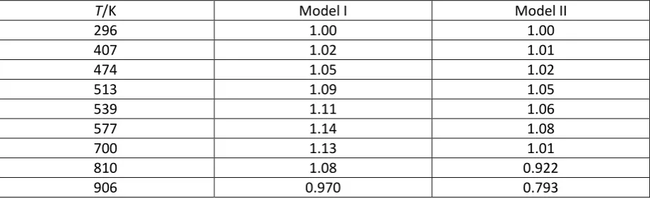
Table S1. Correction factors for rate coefficients based on the absorption cross sections derived in

Section 2. The rate coefficients obtained by absorption spectroscopy, and tabulated in Table II of

Slagle et al.,2 were multiplied by the factors given below to correct for errors in the absorption cross

sections used in the paper. The temperature dependent factors needed for a 0.6 nm bandpass are

included (see Section 2)

T/K Model I Model II

296 1.00 1.00

407 1.02 1.01

474 1.05 1.02

513 1.09 1.05

539 1.11 1.06

577 1.14 1.08

700 1.13 1.01

810 1.08 0.922

[image:2.595.69.529.608.749.2]

(3)

3. The results of fitting the data used in Fit 5, but with different energy transfer parameters above and below 1000 K. degree of freedom) is essentially the same as in Table 3, fit 5.

Energy transfer parameters 300 1000 K

Tref = 298 K; <E>down,ref = 282 cm-1, m = 0.65

Energy transfer parameters 1350 K 2034 K.

Tref = 1400 K; <E>down,ref = 677 cm-1, m = -0.09

Golden11 fitted the data of Slagle et al.2 and Oehlschlaeger et al.4 using a stochastic master equation,

with k(E) calculated with a Gorin model, constrained to the k (T) values of Klippenstein et al..12 He

obtained significantly lower values of <E>down for Ar, increasing from 10 cm-1 at 296 K to 233 cm-1

at 1924 K. He also found that <E>down increased more rapidly with T for T<1000 K than it did for

T>1000K. The parameters shown above give <E>down reaching a maximum of 677 cm-1 at 1400 K

and then decreasing slightly with increasing temperature. The reason for the lower values for the

energy transfer parameters from the fits by Golden, especially at low T is not clear but indicates

smaller values for k(E) using the Gorin model compared with those from the ILT fits used here. These

differences could derive from the different treatments of the rotational degrees of freedom in the

transition state (all implicitly active in the ILT method, only the K-rotor active in the Gorin model).

4. The results of extending the data used in Fit 5 to include the experimental data of Du et al.3

Figure S1 shows a plot of the experimental values vs the calculated values for Fit 5 and also includes

the experimental data of Du et al.3 The insert expands the low pressure region and shows that the

data from Du et al. fall systematically below the best fit line and show more scatter than do the data

(4)

[image:4.595.119.464.101.376.2]

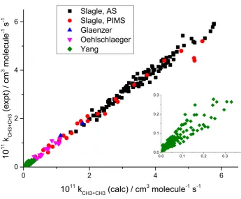
Figure S1. Plot of the experimental rate coefficients in Ar vs the best fit values from the master equation, including the high temperature data of Du et al.3 The data refer to: Slagle et al.,2 Glänzer et al.,5 Du et al.,3 Oehlschlaeger et al.4

5. The results of extending the data used in Fit 5 to include the experimental data of Yang et al.6

Figure S2 shows a plot of the experimental values vs the calculated values for Fit 5 and also includes

the experimental data of Yang et al.6 The latter were fitted using independent energy transfer

parameters for Kr. The resulting parameters are:

(5)

[image:5.595.119.465.95.381.2]

Figure S2. Plot of the experimental rate coefficients vs the best fit values from the master equation. The figure includes data in Ar (c.f. Figure S1, omitting the data of Du et al.3) and data in Kr (Yang et al.6). The Kr data have been fitted with the same ILT parameters as the Ar data, but with

(6)

6. Limiting zero pressure rate coefficients, k0(T)/ cm 6

molecule-2 s-1

T/K Fit 5 Fit 6 Baulch et al. (ref)

300 1.224E-25 8.348E-26 1.556E-26

400 2.824E-26 2.378E-26 6.614E-27

500 1.054E-26 7.845E-27 2.779E-27

600 3.354E-27 2.872E-27 1.233E-27

700 1.335E-27 1.136E-27 5.834E-28

800 5.381E-28 4.229E-28 2.937E-28

900 2.292E-28 1.890E-28 1.562E-28

1000 9.460E-29 7.461E-29 8.718E-29

1100 4.766E-29 3.630E-29 5.076E-29

1200 3.153E-29 1.808E-29 3.067E-29

1300 1.103E-29 9.175E-30 1.915E-29

1400 5.751E-30 4.746E-30 1.230E-29

1500 2.705E-30 2.488E-30 8.109E-30

Parameterized form of k0 = A × (T/298) -n

× exp(-C/T_{) cm}6_molecule-2_s-1

Fit 5 (Ar) A = 1.599 × 10-22 n = 10.03 C = 2191

Fit 6 (Ar) A = 1.365 × 10-22 n = 10.04

C = 2227

Broadening parameters based on Troe and Ushakov7

For M , Troe and Ushakov give

with

where ln⁡ , the parameter is in the range 0.9 1.1 and b is in the range 0.1 0.25

Fitting the fall off data from the best-fit master equation output to these expressions, with

⁡and⁡ fixed at the values derived from the master equation analysis (sections 5.1 and 5.2 in the main paper) and fitting to only Fcent, ⁡and⁡ gave the required Fcent in the form Aexp(-BT) + C with

Fit 5 (Ar) A = 0.151 B = 0.0029 K-1 C = 0.0497

b = 0.25 = 1.03

Fit 6 (Ar) A = 0.135 B = 0.0022 K-1 C = 0.050

(7)

= 1.1

[image:7.595.108.458.167.434.2]

Figure S3 shows fits to the master equation output using these parameters.

Figure S3. Comparison of the fits to the master equation output using the parameterisation of Troe and Ushakov (red lines) with the master equation output, derived from Fit 6 .

7. Chebyshev polynomials for k(p,T) for CH3 + CH3

This section outlines the basis of fitting the master equation output using Chebyshev

polynomials. Supporting Information II is a spreadsheet that allows the rate coefficient to be

calculated based on these polynomials under any pressure, temperature combination,

within the fitting range. The polynomials only apply within the ranges 200

T

/ K 2000 for

Ar and 200

T

/ K 1000 for He ; 1 × 10

15

[M]

1 × 10

25

/ cm

3

molecule

-1

s

-1

for both Ar

(8)

The Chebyshev

8

representations of the phenomenological rate coefficients are obtained

using the following approach. A particular rate coefficient is represented in the form:



 



NT P

i N

j

j i

ij

T

P

T

k

P

T

k

1 1

)

(

)

(

)]

,

(

log[

)]

,

(

log[





(S1)

where

T

and

P

are transformations of 1/

T

and log(

P

) on the [-1,1] interval and



_i

is a

Chebyshev polynomial of degree

i

. In the current work

N

T and

N

p are chosen to be 10 and 8

respectively giving an expansion of 80 coefficients,



_ij

, which are determined as follows:

)

(

)

(

)]

,

(

log[

0 0

1 1

0 i m j n

d m on d n m d d const

ij

k

T

P

T

P

T P

P

T







 



(S2)

with

       



T m d m T 2 1 2 cos

0

(S3)

       



P m d n P 2 1 2 cos

0

(S4)

























1

1 ,

1

1 ,

1

2

1 ,

4 j

i

j

i

j

i

j

i

const

(S5)

and the number of Chebyshev grid points,

d

T,

d

P is chosen to be 10 and 8 respectively.

(9)

Fit 5, Ar

Fit 6, Ar

Fit, average Ar:A = 5.76e-11 cm3 molecule-1 s-1 and n = -0.335, ⁡= 295 cm-1, m= 1.38, B = -1.02e-3 K-1

-10.718100 0.681445 -0.332839 0.095192 -0.018289 0.004732 0.000605 -0.001850

0.688996 -0.847133 0.307101 0.004042 -0.042774 0.010897 -0.000133 -0.000971

-0.375683 0.481882 -0.115601 -0.052401 0.031256 0.004865 -0.005578 0.000495

0.213974 -0.265188 0.033189 0.046397 -0.010502 -0.010841 0.002812 0.002058

-0.121564 0.143106 -0.002446 -0.030097 -0.001071 0.008818 0.000826 -0.002286

0.068706 -0.076154 -0.006528 0.016774 0.004906 -0.004927 -0.002484 0.001242

-0.038637 0.040084 0.007371 -0.008377 -0.004919 0.001951 0.002482 -0.000251

0.021552 -0.020837 -0.005801 0.003773 0.003669 -0.000331 -0.001774 -0.000276

-0.011794 0.010608 0.003919 -0.001504 -0.002338 -0.000307 0.001017 0.000418

0.006115 -0.005140 -0.002327 0.000504 0.001301 0.000402 -0.000479 -0.000348

-10.720100 0.651548 -0.325179 0.095516 -0.018035 0.004935 -0.000038 -0.001706

0.731786 -0.819788 0.311798 -0.004804 -0.042172 0.011966 -0.000308 -0.000605

-0.373495 0.460396 -0.118701 -0.048027 0.033326 0.003456 -0.006010 0.000717

0.205423 -0.249977 0.036012 0.043878 -0.012549 -0.010346 0.003620 0.001989

-0.113716 0.133118 -0.005055 -0.028653 0.000557 0.008872 0.000136 -0.002475

0.062858 -0.069902 -0.004340 0.016050 0.003696 -0.005206 -0.002037 0.001521

-0.034641 0.036317 0.005691 -0.008105 -0.004074 0.002286 0.002254 -0.000516

0.018963 -0.018653 -0.004599 0.003746 0.003118 -0.000643 -0.001694 -0.000058

-0.010200 0.009397 0.003119 -0.001580 -0.002003 -0.000056 0.001016 0.000255

0.005212 -0.004514 -0.001847 0.000595 0.001116 0.000229 -0.000504 -0.000241

-10.719100 0.666260 -0.328419 0.094793 -0.017968 0.004875 0.000234 -0.001761

0.712455 -0.836768 0.311040 -0.000776 -0.042379 0.011411 -0.000298 -0.000718

-0.375071 0.471736 -0.117059 -0.050572 0.032426 0.004178 -0.005788 0.000604

0.209521 -0.257209 0.034244 0.045326 -0.011474 -0.010680 0.003210 0.002044

-0.117274 0.137557 -0.003515 -0.029374 -0.000358 0.008889 0.000513 -0.002395

0.065422 -0.072554 -0.005527 0.016331 0.004372 -0.005068 -0.002288 0.001375

-0.036351 0.037861 0.006536 -0.008150 -0.004529 0.002107 0.002375 -0.000365

0.020051 -0.019526 -0.005166 0.003686 0.003402 -0.000481 -0.001724 -0.000186

-0.010862 0.009874 0.003476 -0.001491 -0.002169 -0.000179 0.000999 0.000351

(10)

Fit , average He : A = 5.76e-11 cm3 molecule-1 s-1 and n = -0.335, ⁡= 98 cm-1, m= 1.65, 200 T/ K 1000

(11)

8. MESMER CH3 + CH3 xml Input File9,10

<?xml version="1.0" encoding="utf-8"?>

<?xml-stylesheet type='text/xsl' href='../../mesmer2.xsl' media='other'?> <?xml-stylesheet type='text/xsl' href='../../mesmer1.xsl' media='screen'?> <me:mesmer xmlns="http://www.xml-cml.org/schema"

xmlns:me="http://www.chem.leeds.ac.uk/mesmer"

xmlns:xsi="http://www.w3.org/2001/XMLSchema-instance"> <me:title>CH3 + CH3</me:title>

</property>

</property>

</property>

</property> </propertyList>

<me:DOSCMethod name="QMRotors" />

(12)

</molecule>

</property>

</property>

<me:DOSCMethod name="QMRotors" />

<me:energyTransferModel xsi:type="me:ExponentialDown"> <me:deltaEDown units="cm-1">250</me:deltaEDown> </me:energyTransferModel>

</molecule>

(13)

</property>

</property>

</property>

<me:DOSCMethod>QMRotors</me:DOSCMethod>

<me:ExtraDOSCMethod xsi:type="me:HinderedRotorQM1D"> <me:bondRef>b1</me:bondRef>

<me:HinderedRotorPotential format="numerical" units="cm-1" expansionSize="7" useSineTerms="yes">

(14)

<me:PotentialPoint angle="30" potential= "508"/> <me:PotentialPoint angle="45" potential= "150"/> <me:PotentialPoint angle="60" potential= "0"/> <me:PotentialPoint angle="75" potential= "150"/> <me:PotentialPoint angle="90" potential= "508"/> <me:PotentialPoint angle="105" potential= "864"/> <me:PotentialPoint angle="120" potential= "1011"/> <me:PotentialPoint angle="135" potential= "864"/> <me:PotentialPoint angle="150" potential= "508"/> <me:PotentialPoint angle="165" potential= "150"/> <me:PotentialPoint angle="180" potential= "0"/> <me:PotentialPoint angle="195" potential= "150"/> <me:PotentialPoint angle="210" potential= "508"/> <me:PotentialPoint angle="225" potential= "864"/> <me:PotentialPoint angle="240" potential= "1011"/> <me:PotentialPoint angle="255" potential= "864"/> <me:PotentialPoint angle="270" potential= "508"/> <me:PotentialPoint angle="285" potential= "150"/> <me:PotentialPoint angle="300" potential= "0"/> <me:PotentialPoint angle="315" potential= "150"/> <me:PotentialPoint angle="330" potential= "508"/> <me:PotentialPoint angle="345" potential= "864"/> <me:PotentialPoint angle="360" potential= "1011"/> </me:HinderedRotorPotential>

<me:periodicity>3</me:periodicity> </me:ExtraDOSCMethod>

<me:energyTransferModel xsi:type="me:ExponentialDown">

<me:deltaEDown bathGas="Ar" units="cm-1" >295</me:deltaEDown>

<me:deltaEDownTExponent bathGas="Ar" referenceTemperature="1400" >1.38</me:deltaEDownTExponent>

<me:deltaEDownActivationParam units="K-1" >-0.00102</me:deltaEDownActivationParam>

<me:deltaEDown bathGas="He" units="cm-1" lower="50" upper="400" stepsize="10">98</me:deltaEDown>

<me:deltaEDownTExponent bathGas="He" lower="-2.5" upper="2.5" stepsize="0.01">1.65</me:deltaEDownTExponent>

</me:energyTransferModel>

<me:reservoirSize units="kJ/mol">-250.0</me:reservoirSize> </molecule>

(15)

</property>

</propertyList> </molecule>

</property>

</property>

</property>

(16)

</moleculeList> <reactionList> <reaction id="R1"> <reactant>

<me:excessReactantConc>1e14</me:excessReactantConc>

<me:MCRCMethod name="MesmerILT" xsi:type="MesmerILT">

<me:preExponential lower="1e-11" upper="8e-11" stepsize="1e-13">5.763e-11</me:preExponential>

<me:activationEnergy>0.0</me:activationEnergy> <me:TInfinity>298.0</me:TInfinity>

<me:nInfinity lower="-0.9" upper="0.9" stepsize="0.005">-0.335</me:nInfinity> </me:MCRCMethod>

</reaction> </reactionList> <me:conditions>

<me:bathGas>Ar</me:bathGas> <me:PTs>

<me:PTpair units="atm" P= " 2.19E-01 " T= " 1803 " precision="d"> <me:bathGas>Ar</me:bathGas> </me:PTpair>

</me:PTs> </me:conditions> <me:modelParameters>

<me:grainSize units="cm-1">50</me:grainSize>

<me:energyAboveTheTopHill>20.</me:energyAboveTheTopHill> </me:modelParameters>

<me:control>

(17)

<me:MarquardtIterations>12</me:MarquardtIterations> <me:MarquardtTolerance>1e-7</me:MarquardtTolerance> <me:MarquardtDerivDelta>0.025</me:MarquardtDerivDelta> </me:calcMethod-->

<me:testDOS/>

<me:printSpeciesProfile /> <me:testMicroRates/>

<me:printGrainkfE/>

<me:printGrainkbE/>

<me:printSpeciesProfile/> <me:testRateConstants/>

<me:calcMethod xsi:type="me:analyticalRepresentation"> <me:chebNumTemp>11</me:chebNumTemp>

<me:chebNumConc>9</me:chebNumConc> <me:chebMaxTemp>2000</me:chebMaxTemp> <me:chebMinTemp>200</me:chebMinTemp>

<me:chebMaxConc units="PPCC">1E+25</me:chebMaxConc> <me:chebMinConc>1E+15</me:chebMinConc>

<me:chebTExSize>10</me:chebTExSize> <me:chebPExSize>8</me:chebPExSize> </me:calcMethod>

<me:eigenvalues>1</me:eigenvalues> </me:control>

</me:mesmer>

References

(1) Western, C. M. PGOPHER, a Program for Simulating Rotational Structure, Version 8.0, Http://Pgopher.chm.bris.ac.uk, doi:10.5523/Bris.Huflggvpcuc1zvliqed497r2; University of Bristol, 2014.

(2) Slagle, I. R.; Gutman, D.; Davies, J. W.; Pilling, M. J. Study of the Recombination Reaction CH3+CH3 -->C2H6 Part 1. Experiment. J. Phys. Chem.1988, 92, 2455-2462.

(3) Du, H.; Hessler, J. P.; Ogren, P. J. Recombination of Methyl Radicals .1. New Data between 1175 and 1750 K in the Falloff Region. J. Phys. Chem.1996, 100, 974-983.

(4) Oehlschlaeger, M. A.; Davidson, D. F.; Hanson, R. K. High-Temperature Ethane and Propane Decomposition. Proceedings of the Combustion Institute2005, 30, 1119-1127.

(5) Glanzer, K.; Quack, M.; Troe, J. Spectroscopic Determination of Methyl Radical Recombination Rate Constant in Shock-Waves. Chem. Phys. Lett.1976, 39, 304-309.

(6) Yang, X. L.; Goldsmith, C. F.; Tranter, R. S. Decomposition and Vibrational Relaxation in CH3I and Self-Reaction of CH3 Radicals. J. Phys. Chem. A2009, 113, 8307-8317.

(7) Troe, J.; Ushakov, V. G. Representation of "Broad" Falloff Curves for Dissociation and Recombination Reactions. Z. Phys. Chemie-Int. J. Res. Phys. Chem. Chem. Phys.2014, 228, 1-10.

(8) Naik, C.; Carstensen, H. H.; Dean, A. M. Reaction Rate Representation Using Chebyshev Polynomials. In Spring Meeting of the Combustion Institute,

(18)

(9) Glowacki, D. R.; Liang, C. H.; Morley, C.; Pilling, M. J.; Robertson, S. H. MESMER: An Open-Source Master Equation Solver for Multi-Energy Well Reactions. J. Phys. Chem. A2012, 116, 9545-9560.

(10) Robertson, S. H.; Glowacki, D. R.; Liang, C.-H.; Morley, C. M.; Pilling, M. J. MESMER (Master Equation Solver for Multi-Energy Well Reactions); an Object Oriented C++ Programme for Carrying out Master Equation Calculations and Analysis on Arbitrary Multiple Well Systems.;

http://sourceforge.net/projects/mesmer, 2009.

(11) Golden, D.M. What Do We Know About the Iconic System CH3+CH3+M C2H6+M?,

Z. Phys. Chem.2011, 225, 969-982