Recommending Structured Objects: Paths and Sets

Paths and Sets

Dawei Chen

A thesis submitted for the degree of

Doctor of Philosophy of

The Australian National University

The majority of the work in this thesis has been published in conference proceedings and preprints, I list them below.

• Dawei Chen, Cheng Soon Ong, Lexing Xie.

Learning points and routes to recommend trajectories.

InProceedings of the ACM Conference on Information and Knowledge Management, pages 2227–2232. 2016.

• Dawei Chen, Dongwoo Kim, Lexing Xie, Minjeong Shin, Aditya Krishna Menon,

Cheng Soon Ong, Iman Avazpour, John Grundy.

PathRec: Visual analysis of travel route recommendations.

InProceedings of the ACM Recommender Systems Conference, pages 364–365. 2017.

• Aditya Krishna Menon,Dawei Chen, Lexing Xie, Cheng Soon Ong.

Revisiting revisits in trajectory recommendation.

InProceedings of the International Workshop on Recommender Systems for Citizens, pages 2:1–2:6. 2017.

• Dawei Chen, Lexing Xie, Aditya Krishna Menon, Cheng Soon Ong.

Structured recommendation.

CoRR, abs/1706.09067. 2017. https://arxiv.org/abs/1706.09067

• Dawei Chen, Cheng Soon Ong, Aditya Krishna Menon. Cold-start playlist recommendation with multitask learning.

CoRR, abs/1901.06125. 2019. https://arxiv.org/abs/1901.06125

Except where otherwise indicated, this thesis is my own original work.

Principal Research Scientist, Data61, CSIRO

Adjunct Associate Professor, The Australian National University Canberra, ACT, Australia

Associate Supervisors

Lexing Xie

Professor, The Australian National University Canberra, ACT, Australia

Aditya Krishna Menon

Honorary Senior Lecturer, The Australian National University Senior Research Scientist, Google

First, I would like to express my deepest gratitude to my primary supervisor, Dr. Cheng Soon Ong, for his inspiration and guidance during my doctoral study. I greatly appreciate his tireless efforts for helping me formulate my research problems as well as guiding me towards making good decisions among the exponential number of possible design choices. This thesis would not be possible if not for his dedication. I would like to sincerely thank my associate supervisor, Dr. Lexing Xie, for her support of my PhD application and her invaluable guidance during the past few years. I greatly appreciate her help in presenting my work in CIKM when my visa was granted too late to attend the conference. My sincere thanks also goes to my associate supervisor, Dr. Aditya Krishna Menon, for contributing a large number of hours to help with my research, including but not limited to deriving equations, editing paper drafts and challenging me to prove theorems. His style of working from the most basic principles has always been inspiring to me.

I would also like to thank all members in the ANU Computational Media Lab for organising various fun group activities and social events. I am indebted to the Australian National University, NICTA and CSIRO Data61 for providing financial and technical support for my research. Last but not the least, I want to thank my family for their encouragement and constant support.

Recommender systems have been widely adopted in industry to help people find the most appropriate items to purchase or consume from the increasingly large collection of available resources (e.g., books, songs and movies). Conventional recommendation techniques follow the approach of “ranking all possible options and pick the top”, which can work effectively for single item recommendation but fall short when the item in question has internal structures. For example, a travel trajectory with a sequence of points-of-interest or a music playlist with a set of songs. Such structured objects pose critical challenges to recommender systems due to the intractability of ranking all possible candidates.

This thesis study the problem of recommending structured objects, in particular, the recommendation of path (a sequence of unique elements) and set(a collection of distinct elements). We study the problem of recommending travel trajectories in a city, which is a typical instance of path recommendation. We propose methods that combine learning to rank and route planning techniques for efficient trajectory recommendation. Another contribution of this thesis is to develop the structured recommendation approach for path recommendation by substantially modifying the loss function, the learning and inference procedures of structured support vector machines. A novel application of path decoding techniques helps us achieve efficient learning and recommendation. Additionally, we investigate the problem of recom-mending a set of songs to form a playlist as an example of the set recommendation problem. We propose to jointly learn user representations by employing the multi-task learning paradigm, and a key result of equivalence between bipartite ranking and binary classification enables efficient learning of our set recommendation method. Extensive evaluations on real world datasets demonstrate the effectiveness of our proposed approaches for path and set recommendation.

Declaration iii

Acknowledgement ix

Abstract xi

List of Figures xviii

List of Tables xix

1 Introduction 1

1.1 Motivation . . . 1

1.2 Contributions . . . 2

1.3 Thesis outline . . . 4

2 Background 5 2.1 The problem of recommending structured objects . . . 5

2.1.1 Path recommendation . . . 6

2.1.2 Set recommendation . . . 7

2.2 Techniques for recommender systems . . . 7

2.2.1 Recommendation strategies . . . 7

2.2.2 Matrix factorisation techniques . . . 8

2.3 Structured prediction . . . 11

2.3.1 Structured support vector machines . . . 11

2.3.2 Methods to train the SSVMs . . . 14

2.4 Path decoding in Markov chains . . . 17

2.4.1 The forward and backward approaches in HMM . . . 18

2.4.2 The list Viterbi algorithm . . . 22

2.4.3 Sub-tour elimination in s-t path TSP . . . 26

2.4.4 Heuristic algorithms . . . 27

2.5 Binary classification and bipartite ranking . . . 28

2.5.1 Loss functions for binary classification . . . 28

2.5.2 Loss functions for bipartite ranking . . . 29

2.6 Multi-task learning . . . 31

2.7 Summary . . . 32

3 Feature-based Travel Trajectory Recommendation 33 3.1 Introduction . . . 33

3.2 Problem statement . . . 35

3.3 Related work . . . 35

3.3.1 Solutions for typical travel recommendation problems . . . 36

3.3.2 Methods for ranking locations and trajectories . . . 36

3.3.3 Features and information employed . . . 37

3.4 Query features and POI transition . . . 37

3.5 Tour recommendation . . . 39

3.5.1 POI ranking and route planning . . . 39

3.5.2 Combining ranking and transition . . . 40

3.5.3 Avoiding sub-tours . . . 41

3.5.4 Incorporating time constraints . . . 43

3.5.5 Discussion . . . 43

3.5.6 Measuring performance . . . 44

3.6 Experiments . . . 45

3.6.1 Photo trajectories from five cities . . . 45

3.6.2 Experimental setup . . . 46

3.6.3 Results . . . 47

3.6.4 An illustrative example . . . 49

3.7 Summary . . . 50

4 Structured Recommendation for Travel Trajectories 51 4.1 Introduction . . . 51

4.2 Problem statement . . . 52

4.3 A structured recommendation approach . . . 53

4.3.1 Trajectory recommendation as structured prediction . . . 53

4.3.2 Global cohesion and the SP model . . . 54

4.3.3 Multiple ground truths and the SR model . . . 54

4.3.4 Eliminating loops in recommendation . . . 55

4.3.5 SP and SR model training . . . 56

4.3.6 Discussion . . . 57

4.3.7 Summary of proposed methods . . . 59

4.4 Experiments . . . 59

4.4.2 Evaluation setting . . . 60

4.4.3 Results and discussion . . . 62

4.4.4 A qualitative example . . . 65

4.5 Related work . . . 66

4.6 Summary . . . 67

5 Music Playlist Recommendation with Multi-task Learning 69 5.1 Introduction . . . 69

5.2 Problem statement . . . 70

5.3 Related work . . . 72

5.3.1 Playlist recommendation . . . 73

5.3.2 Cold-start recommendation . . . 73

5.3.3 Connections between bipartite ranking and binary classification 74 5.4 Multi-task learning for playlist recommendation . . . 74

5.4.1 Multi-task learning objective . . . 75

5.4.2 Cold-start playlist recommendation . . . 76

5.4.3 Ranking songs via Bottom-Push . . . 77

5.4.4 Efficient optimisation . . . 78

5.5 Experiments . . . 79

5.5.1 Dataset . . . 79

5.5.2 Features . . . 80

5.5.3 Experimental setup . . . 81

5.5.4 Results . . . 85

5.6 Discussion . . . 91

5.6.1 Multi-task learning, bipartite ranking and binary classification . 91 5.6.2 Cold-start playlist recommendation versus playlist continuation 92 5.6.3 Information of songs, playlists and users . . . 92

5.7 Summary . . . 93

6 Conclusion 95 6.1 Research summary . . . 95

6.2 Future work . . . 96

A Cutting-plane Methods 97 A.1 Overview of cutting-plane methods . . . 97

A.2 Methods to generate query points . . . 99

A.2.1 Method of Kelley-Cheney-Goldstein . . . 100

A.2.2 Chebyshev centre method . . . 100

A.2.4 Centre of gravity or Bayes point method . . . 101

B Linking Losses for Bipartite Ranking and Binary Classification 103 C Time Constraints for Travel Trajectory Recommendation 107 D Details of Travel Trajectory Recommendation Experiments 111 D.1 Features . . . 111

D.1.1 POI-query features . . . 111

D.1.2 Transition features . . . 111

D.2 Evaluation metrics . . . 112

D.2.1 F1score on points . . . 113

D.2.2 F1score on pairs . . . 113

D.2.3 Kendall’stwith ties . . . 114

D.3 Additional empirical results . . . 114

E Proof of Lemma 1 121

2.1 Illustration of Matrix Factorisation. . . 9

2.2 Graphical models of PMF and BPMF. . . 10

2.3 Graphical model of a hidden Markov model (HMM). . . 18

3.1 Three settings of travel recommendation problems. . . 34

3.2 Transition matrices for two POI features. . . 39

3.3 Examples of F1versus pairs-F1 as evaluation metric. . . 45

3.4 Example of recommendations from different methods. . . 50

4.1 Histograms of the number of trajectories per query. . . 60

4.2 Histograms of trajectory length. . . 60

4.3 F1 score on points for short and long trajectories on Glasgow. . . 64

4.4 F1 score on pairs for short and long trajectories on Glasgow. . . 64

4.5 Kendall’stfor short and long trajectories on Glasgow. . . 64

4.6 Example of a recommended trajectory. . . 65

5.1 Three settings of cold-start playlist recommendation. . . 70

5.2 Histogram of the number of playlists per user. . . 81

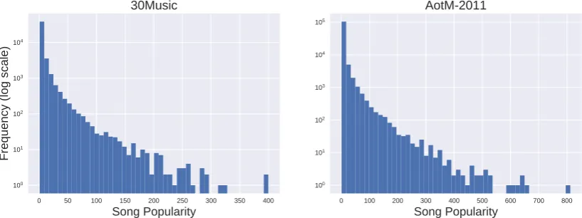
5.3 Histogram of song popularity. . . 81

5.4 Illustration of a non-linear transformation for Novelty and Spread. . . . 85

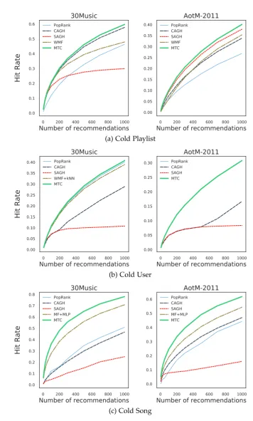
5.5 Hit Rate of playlist recommendation in three cold-start settings. . . 86

5.6 Raw Novelty of playlist recommendation in three cold-start settings. . . 89

A.1 Illustration of cutting-plane methods. . . 98

D.1 F1 score on points for trajectories on Osaka. . . 117

D.2 F1 score on pairs for trajectories on Osaka. . . 117

D.3 Kendall’stfor trajectories on Osaka. . . 117

D.4 F1 score on points for trajectories on Toronto. . . 118

D.5 F1 score on pairs for trajectories on Toronto. . . 118

D.6 Kendall’stfor trajectories on Toronto. . . 118

D.7 F1 score on points for trajectories on Edinburgh. . . 119

D.8 F1 score on pairs for trajectories on Edinburgh. . . 119

D.9 Kendall’stfor trajectories on Edinburgh. . . 119

D.10 F1 score on points for trajectories on Melbourne. . . 120

D.11 F1 score on pairs for trajectories on Melbourne. . . 120

2.1 Techniques for recommending structured objects. . . 6

2.2 Time and space complexities of three typical list Viterbi algorithms. . . 26

3.1 Statistics of trajectory datasets. . . 46

3.2 Information captured by different trajectory recommendation methods. 46 3.3 Performance comparison in terms of F1scores. . . 48

3.4 Performance comparison in terms of pairs-F1scores. . . 48

4.1 Challenges of travel trajectory recommendation and proposed solutions. 52 4.2 Summary of challenges considered in different methods. . . 59

4.3 Statistics of trajectory datasets. . . 60

4.4 F1 score on points of trajectory recommendation methods. . . 63

4.5 F1 score on pairs of trajectory recommendation methods. . . 63

4.6 Kendall’stof trajectory recommendation methods. . . 63

5.1 Glossary of frequently used symbols. . . 72

5.2 Methods to rank songs in three cold-start settings. . . 76

5.3 Statistics of music playlist datasets. . . 80

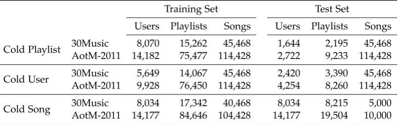
5.4 Statistics of datasets in three cold-start settings. . . 82

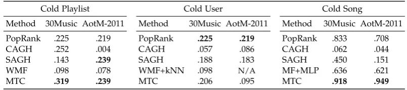
5.5 AUC for playlist recommendation in three cold-start settings. . . 85

5.6 Raw Spread for playlist recommendation in three cold-start settings. . . 88

5.7 Transformed Spread for cold-start playlist recommendation. . . 88

5.8 Transformed Novelty for cold-start playlist recommendation. . . 90

D.1 Features of POI with respect to query. . . 112

D.2 POI features used to capture POI-POI transitions. . . 112

D.3 Performance of trajectory recommendation on best of top-1. . . 115

D.4 Performance of trajectory recommendation on best of top-3. . . 115

D.5 Performance of trajectory recommendation on best of top-5. . . 116

D.6 Performance of trajectory recommendation on best of top-10. . . 116

Introduction

The ever increasing number of available items from content providers (e.g., news articles and blog posts from online publishing platforms, books from Amazon book store, music from Spotify and Apple Music, and movies from Netflix library) pose critical challenges for both users and content providers. This information overload problem makes it particularly difficult for users to find items they want, and further, it undermines the effort to facilitate users getting the most appropriate items that content providers have tirelessly been striving to achieve. Such challenges motivate the development ofrecommender system, a type of information system that suggests items which (hopefully) match users’ preferences. Good recommendations enhance user satisfaction (Bennett et al., 2007; Koren et al., 2009; Aggarwal, 2016), which helps content providers to be more successful, and therefore enables the further expansion of available items to attract even more users. This in turn makes it more challenging to provide good recommendations that meet user needs.

1

.

1

Motivation

Classic recommender systems (e.g., those used for book or movie recommendation) work by ranking items for a particular user. One of the most widely used techniques for recommender systems of this type is the collaborative filtering approach (Goldberg et al., 1992), in particular, latent factor models such as the matrix factorisation family of techniques (Koren et al., 2009). These methods work by explicitly matching user preferences with item properties, both of which are latent factors learned from historical interaction records between users and items (e.g., user’s ratings of items, histories of purchases or browsing). The advantage of this technique is the ability to automatically learn informative representations of users and items from historical data, and the capability to scale to large systems with millions of users and items, and some variants can even capture the temporal dynamics of user preferences (Koren et al., 2009; Koren, 2009; Rendle et al., 2010; Xiong et al., 2010).

However, there are at least two limitations of such approaches. First, it suffers from addressing users or items without historical records, since it is unlikely to learn any meaningful representations for these new users and items; this is known as the

cold startproblem (Schein et al., 2002; Koren et al., 2009). Further, this approach makes a recommendation for a user by scoring each item for that user and suggests the top scored ones, which falls short when dealing with structured objects (i.e., object that is a cohesive composition of interrelated and interdependent elements) effectively, since the huge number of possible combinations of elements is unlikely to be scored efficiently if one adopts a naïve approach (Taskar, 2004; Joachims et al., 2009b).

On the other hand, the task of recommending structured objects is prevalent in real-world applications, for example, recommending a trajectory of points-of-interest (POIs) in a city to a visitor (Lu et al., 2010, 2012; Lim et al., 2015; Chen et al., 2016; He et al., 2018), suggesting a chemical compound (Dehaspe et al., 1998; Agrafiotis et al., 2007), or a playlist of songs (McFee and Lanckriet, 2011; Chen et al., 2012; Choi et al., 2016; Ben-Elazar et al., 2017). A trajectory is a sequence of distinct POIs, which is a

path; and a music playlist involves asetof unique songs. Such tasks of recommending structured objects (e.g., paths and sets), which are both practically important and computationally hard, motivate the work in this thesis.

1

.

2

Contributions

In this thesis, we develop techniques that can efficiently recommend objects with different types of structures, in particular,pathsandsets. Machine learning techniques including learning to rank and structured prediction, as well as route planning techniques are employed to achieve efficient path recommendation. We empirically evaluate these techniques on the task of recommending travel trajectories. In addition, we develop a technique for set recommendation by leveraging bipartite ranking and multi-task learning, and evaluate it on the task of recommending a set of songs from a music library. The major contributions of this thesis are summarised as follows:

can efficiently recommend travel trajectories by employing the RankSVM (Lee and Lin, 2014; Kuo et al., 2014) and route planning techniques from the research of the TSP or the orienteering problem (Miller et al., 1960; Golden et al., 1987; Applegate et al., 2011). This work is published in Chen et al. (2016).

2. Structured recommendation for paths based on structured prediction. We study the problem of recommending paths from a structured prediction perspec-tive (Tsochantaridis et al., 2004; Taskar et al., 2005; BakIr et al., 2007; Joachims et al., 2009b), and propose a new structured recommendation approach based on the structured support vector machines (SSVMs) framework. We analyse the fundamental challenges of travel trajectory recommendation, which are shared among many path recommendation tasks, and show how the structured recommendation approach can address these challenges by systematically incor-porating point preferences and transition patterns, as well as a novel application of the list variant of the Viterbi decoding algorithm for hidden Markov mod-els (Soong and Huang, 1991; Seshadri and Sundberg, 1994; Nill and Sundberg, 1995; Nilsson and Goldberger, 2001), or the integer linear programming for-mulation of the s-t pathTSP (Hoogeveen, 1991; An et al., 2015). This work is presented in Chen et al. (2017a,b) and Menon et al. (2017).

3. Efficient set recommendation via bipartite ranking and multi-task learning.

We study the problem of recommending sets, which is to recommend a collection of distinct elements where no particular order of the elements are of interest. We propose a new approach for set recommendation via bipartite ranking (Agarwal and Niyogi, 2005; Ertekin and Rudin, 2011; Menon and Williamson, 2016). Specif-ically, we investigate the problem of recommending a set of songs from a music library to form a new playlist or extend a user’s existing playlist in cold-start scenarios. A bipartite ranking loss is adopted to encourage songs in a playlist to be ranked higher than those not in it, and the multi-task learning paradigm is employed to jointly learn user representations that facilitate cold-start rec-ommendation. Lastly, we achieve efficient learning of the set recommendation approach by leveraging a key equivalence between bipartite ranking and binary classification (Ertekin and Rudin, 2011; Menon and Williamson, 2016). This work is presented in Chen et al. (2019).

1

.

3

Thesis outline

The rest of this thesis is outlined as follows. In Chapter 2, we first define the problem of recommending structured objects. In particular, the problems of interest in this thesis, i.e., the path and set recommendation problems are formulated. We then present classic techniques for recommender systems, and review essential techniques that help us achieve efficient recommendation of paths and sets, including structured prediction and path decoding techniques in Markov chains for path recommendation; and loss functions of bipartite ranking and binary classification as well as the multi-task learning paradigm that enables effective set recommendation.

In Chapter 3, we study the problem of recommending path by investigating one particular example – travel trajectory recommendation, which is to suggest a sequence of points-of-interest (POIs) without repetition. We first show that both the ranking of POIs and the transition patterns between POIs are helpful in recommending travel trajectories, and then present a method that combines POI ranking and route planning to achieve effective recommendation of travel trajectories.

We continue the study of the path recommendation problem in Chapter 4. Here we investigate the travel trajectory recommendation problem from a structured pre-diction viewpoint. We propose the structured recommendation approach for path recommendation by modifying the loss function of the SSVMs to aggregate multiple ground truths for a query. Further, we show how a novel application of the list variant of the classic Viterbi algorithm in both training and inference procedures of the SSVMs can help us overcome the challenges of trajectory recommendation.

In Chapter 5, we study the problem of recommending sets. We investigate an instance of this problem, which is to recommend a set of songs from a music library to form a new playlist or extend an existing playlist in cold-start scenarios. We employ a bipartite ranking loss to rank songs in a playlist above those that are not in it, and adopt the multi-task learning paradigm to learn the representations of all users jointly. A key equivalence between bipartite ranking and binary classification enables the efficient learning of our set recommendation approach from historical playlists.

Background

We review important problems and techniques that serve as the foundation of our work in this thesis. First, we define the problem of recommending structured objects, in particular, we formulate the path and set recommendation problems (Section 2.1). We then review classic techniques for recommender systems (Section 2.2). In Sec-tions 2.3 and 2.4, we present structured prediction and path decoding techniques that enables efficient path recommendation, followed by techniques for set recommen-dation including bipartite ranking and binary classification (Section 2.5), as well as the multi-task learning paradigm (Section 2.6). Table 2.1 shows the corresponding problems and chapters of this thesis that make use of the techniques we reviewed.

2

.

1

The problem of recommending structured objects

The problem of recommendation is to suggest items (e.g., books, movies and news) that a user may like. In this thesis, we consider the case when the item in question is an object with internal structures (i.e., object that is a cohesive composition of interrelated and interdependent elements), such as a set or a tree.

Let Y be the space of all structured objects, given a set ofN queriesthat describe the specifications of desired recommendations, and the historical records (e.g., items purchased or consumed by users) of the corresponding queries

S =_{(q(i)_, {y(ij)

}Ni

j=1)}Ni=1, y(ij) 2Y, i2{1, . . . ,N}, j2{1, . . . ,Ni}, (2.1)

where the i-th queryq(i)_{is associated with N}

i 2Z+ objects. The problem of recom-mending structured objectsis to make recommendations for a new query qnot seen in S, in other words, we learn a function f fromS:

f :q!{y(k)_}K

k=1, y(k)2 Y, (2.2)

where K2Z+is the number of structured objects we shall recommend for queryq.

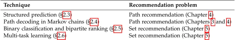
Table 2.1: Techniques for recommending structured objects.

Technique Recommendation problem

Structured prediction (§2.3) Path recommendation (Chapter 4)

Path decoding in Markov chains (§2.4) Path recommendation (Chapters 3 and 4)

Binary classification and bipartite ranking (§2.5) Set recommendation (Chapter 5)

Multi-task learning (§2.6) Set recommendation (Chapter 5)

Compared to standard supervised learning, there are multiple ground truth labels (i.e., recommended objects) in the training set (2.1). Further, in contrast to a fixed set of individual items, the huge number of all possible structured labels (i.e.,|Y|) poses a critical challenge to efficient recommendation. Lastly, taking into account constraints inherent to particular types of structures, for example, asetshould not have duplicate elements, presents another fundamental challenge.

This thesis aims to develop methods that can address these challenges in recom-mending structured objects, particularly for two types of structures: pathandset. We remark that the recommendation of other types of structures (e.g., tree or graph) are important research topics on their own, and we leave them as future work.

2.1.1 Path recommendation

We define apathas a sequence of elements where no element in the sequence appears more than once. The path recommendation problem is a particular instance of the problem of recommending structured objects, where the objects in question are paths. Specifically, given a set of elementsP, a structured object in both (2.1) and (2.2) is a

pathwith elements from_P, i.e.,

y2P|y| andyl 6=yl0, l,l0 2{1, . . . ,|y|},l6=l0,

where |y|denotes the number of elements in pathy.

2.1.2 Set recommendation

A set is a collection of distinct elements, i.e., no element in the collection appears more than once, and there is also no particular order between elements. The set recommendation problem is another example of the problem of recommending structured objects, where the objects in question are sets. In particular, given a set of elementsC, the structured object spaceY in (2.1) and (2.2) is the power set ofC.

In Chapter 5, we study an instance of the set recommendation problem – music playlist recommendation,1_{where we recommend a set of songs from a music library} to form a new playlist or extend a user’s existing playlist, with respect to certain properties specified in a query. We discuss a set recommendation method for music playlist recommendation in three cold-start settings. Our approach employs the multi-task learning paradigm (Section 2.6) to jointly learn user representations, and efficient learning of our set recommendation method is achieved by leveraging a key equivalence between bipartite ranking and binary classification (Section 2.5).

2

.

2

Techniques for recommender systems

In this section, we review classic techniques underlying typical recommender systems (also known as recommendation systems). First, we present the general recommenda-tion strategies, then we review a family of techniques widely employed in practice.

2.2.1 Recommendation strategies

To suggest items to a user, a recommender system generally ranks items by matching their properties with the preferences of the user, and top-ranked items are then recommended. User preferences and item properties are often encoded using a vector of real numbers, which are known as the representation or features of a user or an item. Features can be extracted either manually by human experts (e.g., the Music Genome Project that powers the Pandora Radio (John, 2006)) or learned automatically by computer algorithms. The former is known as thecontent filteringapproach, and the latter is known as thecollaborative filteringapproach (Goldberg et al., 1992), including, for example, the neighbourhood method and latent factor models.

Content filtering approaches rely on human experts to extract (user or item) features, with the advantage of leveraging knowledge accumulated in a certain

domain; however, different experts may devise different values for a certain feature of the same user or item due to the variety in backgrounds and experiences of human experts. In addition, this approach cannot be applied on a large scale simply because the number of human experts in a certain domain is limited.

On the other hand, collaborative filtering approaches leverage historical interaction data to make recommendations. For example, the neighbourhood method makes recommendations by using information from similar users and similar items:2 _{for a} particular useru, it recommends items purchased by users similar tou, or suggests items similar to whatuhas purchased. Latent factor models, on the other hand, learn user and item features (i.e., latent factors) from data of interactions between users and items. For example, learning a low-rank matrix that approximates to the matrix of user-item interactions (e.g., ratings), which is generally very sparse, by exploiting the redundancies in interaction data (Aggarwal and Parthasarathy, 2001).

A major drawback of collaborative filter approaches is the inability to address the

cold-startscenarios, where there is no historical data for either users or items, which occurs when new users or new items are added to an existing system (Koren et al., 2009; Aggarwal, 2016). In this case, the content filtering approach can generally work more effectively as it can leverage external information of the new users or items provided by human experts.

2.2.2 Matrix factorisation techniques

One of the most successful latent factor models is the matrix factorisation (MF) family of techniques, these learn the representation or features of users and items by factorising a matrix with historical records, e.g., ratings of books or movies.

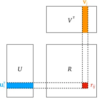
Given a set of Nusers and a set of Mitems, Matrix Factorisation approximates the user-item rating matrixR2RN⇥M using the product of two low rank matrices, i.e., ˆR=UVT, as illustrated in Figure 2.1, whereU2 RN⇥D _{andV 2R}M⇥D _{are low}

rank matrices, with row vectorsui,i2{1, . . . ,N}andvj, j2{1, . . . ,M}representing

theDdimensional latent features of useriand item jrespectively.

Due to the fact that the rating matrix R is generally highly sparse (i.e., most of the entries in R are not observed), classic matrix decomposition methods such as the Singular Value Decomposition (SVD) are not applicable.3 _{In addition, data} imputation could be very costly given the large number of unobserved ratings in

2_{A useruis regarded to be similar to another useru}0_{if bothuandu}0_{have purchased (or have given} similar ratings to) the same set of items, in other words,uandu0_{are like-minded users; similarly, an} itemvis regarded to be similar to another itemv0 _{if bothvandv}0_{have been purchased by (or have} received similar ratings from) the same user.

R

v

V

U

j

ui rij

T

T

Figure 2.1: Illustration of Matrix Factorisation. Uis a matrix of latent factors of users,

V is a matrix of latent factors of items, andRis the observed (sparse) rating matrix. Matrix Factorisation aims to approximate the observed ratings using a function of the corresponding latent factors of users and items, e.g.,rij ⇡u>i vj.

practical datasets, and inaccurate imputation could considerably distort the data. As a result, many works propose to model the observed ratings directly by minimising a regularised squared error (Paterek, 2007; Takács et al., 2007; Koren et al., 2009),

min

U,V N

Â

Â

rij u>i vj

⌘2

+C

N

Â

i=1k

uik2+ M

Â

j=1k

vjk2

!

, (2.3)

wheredij indicates whether userihas rated item j(i.e., dij =1 if entryrij is observed

anddij =0 otherwise), andC2 R+is a regularisation constant.

The objective in Equation (2.3) is non-convex, which makes it hard to find an optimal solution of the problem. However, optimisation methods such as stochastic gradient descent (SGD) and coordinate descent (e.g., alternating least squares (ALS)) have been shown to work effectively in practice (Hu et al., 2008; Koren et al., 2009).

Probabilistic Matrix Factorisation (PMF) (Salakhutdinov and Mnih, 2008b) provides a probabilistic explanation to the regularisation in Equation (2.3). PMF models the user-item rating Rij using a Gaussian random variable, with mean µij = u>i vj and

precisiona. Assuming zero mean spherical Gaussian priors over the latent feature

vectors of both users and items, it has been shown that maximising the log-posterior overUandVis equivalent to

min

U,V N

Â

Â

rij u>i vj

⌘2

+ aU

a N

Â

i=1k

uik2+ a_aV M

Â

j=1k

vjk2, (2.4)

whereaU andaV are hyper-parameters. Figure 2.2(a) shows the graphical model of

ui

vj

r

r

vj ui

Figure 2.2: Graphical models of (a) Probabilistic Matrix Factorisation (PMF) and (b) Bayesian Probabilistic Matrix Factorisation (BPMF). Shaded nodes: observed variables; unshaded nodes: latent variables (Salakhutdinov and Mnih, 2008a).

One approach to tune the hyper-parametersa,aU andaV in Equation (2.4) is to

search over a set of carefully selected values based on the model performance on a validation set, however, this is computationally expensive as a large number of models should to be trained. Alternatively, one can take a Bayesian approach, i.e., introducing priors for hyper-parameters. Salakhutdinov and Mnih (2008a) proposed the Bayesian Probabilistic Matrix Factorisation (BPMF) which assumes more general Gaussian priors over the latent feature vectors of users and items instead of zero mean Gaussian priors as did in the PMF approach,

P(U_|µU,LU) = N

’

i=1N

(ui |µU,L_U1), P(V|µV,LV) =

M

’

j=1N

(vj |µV,LV1).

It further assumes Gaussian-Wishart priors over hyper-parametersQU ={µU,LU}

andQV ={µV,LV},

P(QU |Q0) =N(µU |µ0,(b0LU) 1)W(LU |W0,n0),

P(QV |Q0) =N(µV |µ0,(b0LV) 1)W(LV|W0,n0),

whereQ0={µ0,W0,n0}, andW is the Wishart distribution with degrees of freedom

To obtain the posterior distribution, all model parameters and hyper-parameters need to be integrated out, which is analytically intractable. Salakhutdinov and Mnih (2008a) proposed to approximate the posterior distribution using a Markov chain Monte Carlo (MCMC) method, in particular, a Gibbs sampling algorithm that samples from conditional distributions over model parameters and hyper-parameters.

Matrix factorisation techniques have also been generalised to deal with implicit feedback, e.g., history of purchasing, ad clicking and browsing. Hu et al. (2008) proposed to use a matrix with binary values to represent implicit feedback, and minimised an objective similar to that in Equation (2.3) but with a weighted square loss. Rendle et al. (2009) observed that only positive and unlabelled data are available for implicit feedback, they proposed to dealt with it from a ranking perspective: For a particular user, the approach ranked observed items (e.g., items purchased or viewed by that user) higher than all other items. Other variants of MF that can deal with specific scenarios have been proposed, such as those that can incorporate additional sources of information (Paterek, 2007; Koren, 2008; Koren et al., 2009), and variants that can capture temporal effects (Koren, 2009; Koren et al., 2009; Xiong et al., 2010).

2

.

3

Structured prediction

Structured prediction is the task of predicting interdependent output variables for a given input (BakIr et al., 2007), typical applications including multi-class and multi-label classification, image segmentation and machine translation. The pri-mary challenge in structured prediction is how to make efficient inference in the exponentially-sized output space. In this section, we review an important technique for structured prediction, the structured support vector machines (SSVMs), which generalises the support vector machines (SVMs) to the structured output setting. Another important technique for structured prediction is the conditional random fields (CRFs), Pletscher et al. (2010) proposed a framework that unifies CRFs and SSVMs, we therefore focus on reviewing the SSVMs in this section. In Chapter 4, we formulate the problem of recommending paths in the context of travel trajectories as a structured prediction problem, and adapt both the training and prediction procedures of the SSVMs to deal with challenges in recommending paths.

2.3.1 Structured support vector machines

a particular example x 2 X and a specific structured label y 2 Y. The structured support vector machines makes a prediction given examplexby

y⇤ _=argmax ¯

y2Y

f(x(i), ¯y), (2.5)

which is known as theinferenceor prediction procedure of the SSVMs.

To learn the parameters w, the SSVMs minimises the following (`2 regularised) empirical risk on datasetS ={(x(i),y(i))}N_i=1:

min

w

1

2w>w+

C N

N

Â

i=1

`(y(i)_,f(x(i)_,

·)), (2.6)

where C2R+is a regularisation constant and `(y(i)_,f(x(i)_{,·))is the structured hinge} loss for thei-th labelled example

`(y(i),f(x(i),·)) =max

✓

0, max ¯

y2Y

n

D(y(i), ¯y) (f(x(i),y(i)) f(x(i), ¯y))o◆, (2.7)

hereD(y(i), ¯y)measures the discrepancy between two structured labelsy(i) and ¯y.

If we employ a slack variablex(i)to upper bound the structured hinge loss for the i-th example, we can transform the unconstrained optimisation problem (2.6) into a constrained optimisation problem:

min

w,x 1

2w>w+

C N

N

Â

i=1

x(i)

s.t. x 0,

x(i) D(y(i), ¯y) ⇣f(x(i),y(i)) f(x(i), ¯y)⌘, 8y¯ 2Y.

(2.8)

This formulation is known as the “n-slack” SSVMs due to the number of slack variables in (2.8) equals the numbers of examples N(Joachims et al., 2009a).

We can rearrange the second constraint in problem (2.8) as

x(i)+ f(x(i)_,y(i)_{) D(y}(i)_{, ¯y) + f(x}(i)_{, ¯y),}

8y¯ 2 Y, or equivalently,

x(i)+ f(x(i)_,y(i)_{) max} ¯

y2Y

n

(Equa-tion 2.5). In practice, ifD(y(i), ¯y)can be decomposed into discrepancies of individual

elements iny(i) _{and ¯y, then the loss-augmented inference could be optimised using} techniques similar to that for the inference procedure (2.5).

Joachims et al. (2009a) observed that one can sum up the structured hinge losses (Eq. 2.7) for all examples, which results in the following empirical risk on datasetS:

R(f,S) =max 0, max (y¯(1)_,...,¯y(N)_)2YN

(

1 N

N

Â

i=1 ⇣

D(y(i)_{, ¯y}(i)₎ ⇣_f(x(i)_,y(i)_{) f(x}(i)_{, ¯y}(i)₎⌘⌘

)!

.

(2.10) Similar to the “n-slack” SSVM (2.8), we can transform the (`2regularised) empirical risk minimisation into a constrained optimisation problem, however, here onlyone

slack variable is needed to upper bound the empirical risk R(f,S)defined in (2.10),

min

w,x

1

2w>w+Cx

s.t. x 0,

x 1 N N

Â

D(y(i)_{, ¯y}(i)_{) (f(x}(i)_,y(i)_{) f(x}(i)_{, ¯y}(i)₎₎⌘_,

8(y¯(1), . . . , ¯y(N)₎

2YN. (2.11) This formulation is known as the “1-slack” SSVMs (Joachims et al., 2009a).

If we rearrange the second constraint in (2.11) as

x+ 1

N N

Â

i=1

f(x(i),y(i)) 1

N N

Â

i=1 ⇣

D(y(i), ¯y(i)) + f(x(i), ¯y(i))⌘, 8(y¯(1), . . . , ¯y(N))2YN or equivalently

x+ 1

N N

Â

i=1

f(x(i),y(i)) max

(¯y(1)_,...,¯y(N)_)2YN

1 N N

Â

D(y(i), ¯y(i)) + f(x(i), ¯y(i))⌘. (2.12)

The RHS of Equation (2.12) is known as theloss-augmented inferencein the “1-slack” formulation of the SSVMs.

Both the “n-slack” (2.8) and “1-slack” (2.11) formulations of the SSVMs result in constrained optimisation problems. If the affinity function f(x,y)takes the form of

One practical approach to train both the “n-slack” and “1-slack” formulations of the SSVMs is a cutting-plane method (Joachims et al., 2009a,b), which is a general optimisation technique for constrained optimisation problems with convex objective and constraints (Boyd and Vandenberghe, 2008). Intuitively, it starts with finding an optimal solution by optimising the objective without any constraints, then generating cutting planes (i.e., linear constraints) by querying a cutting-plane oracle (Wulff and Ong, 2013). This procedure is repeated until convergence. In the next section, we review methods to train the SSVMs, in particular, how one can train the “n-slack” and “1-slack” SSVMs efficiently using cutting-plane methods. More details of cutting-plane

methods can be found in Appendix A.

2.3.2 Methods to train the SSVMs

Suppose the affinity function f(x,y)takes the form of a linear function, i.e., f(x,y) =

w>_{Y(x,y)wherewis the parameter vector andY(x,y)is known as thejoint feature}

mapof examplexand structured labely.

Training the n-slack SSVMs To train the “n-slack” SSVMs using cutting-plane methods, we make use of a standard QP solver by repeatedly solving a QP with respect to an increasingly larger set of constraints. In each iteration, a new constraint (or cut) is generated to reduce the feasible region of the problem, until the optimal solution achieves a specified precision#(Joachims et al., 2009b).

Algorithm 1 describes the pseudo-code of a cutting-plane algorithm to train the “n-slack” SSVMs. In each iteration, and for each example, we solve a QP with the current set of constraints_W, the solution is our query pointq(k) _{(Line 5). To check} if the current query point is#-feasible, we first compute the most violated label by

doing the loss augmented inference (Line 7), then check if q(k) _{is#-feasible for this} example (Line 8), if not, we generate a feasibility cut (A.3) and add it to the working setW (Line 9). This procedure is repeated until a#-feasible query point is found.

As a remark, in Algorithm 1 we can compute the structured hinge loss on the fly for each example (Tsochantaridis et al., 2004), i.e.,

x_i(k) =max

✓

0, max ¯

y2Si

n

D(y(i)_{, ¯y) +}

hw(k)_,Y(x(i)_{, ¯y)}

io hw(k)_,Y(x(i)_,y(i)₎

i

◆

,

in this case, the query pointq(k) _=w(k)_.

Algorithm 1 A cutting-plane algorithm to train then-slack SSVMs

1: Input: _{(x(i),y(i)_}iN₌₁, C, #

2: _W =∆, Si = ∆, i2 {1, . . . ,N}, k=1 3: repeat

4: fori=1, . . . ,Ndo

5: Generate query pointq(k) _{= (w}(k)_,x(k)_{)by solving QP (2.8)} w.r.t. all constraints inW

6: .Query the oracle at point q(k) as follows

7: Do loss-augmented inference: ˆ

y(k) _=argmax ¯

y2Y{D(y(i), ¯y) +hw(k),Y(x(i), ¯y)i} 8: ifq(k)is not #-feasible:

hw(k)_,Y(x(i)_,y(i)_{) Y(x}(i)_{, ˆy}(k)_)i+#<D(y(i)_{, ˆy}(k)_{) x}(k)

i then 9: Form afeasibility cutand update constraints:

W =_W[n_hw,Y(x(i)_,y(i)_{) Y(x}(i)_{, ˆy}(k)_{)i D(y}(i)_{, ˆy}(k)_{) x}

i

o

Si =Si[{yˆ(k)}, k= k+1 10: end if

11: end for

12: untilq(k)is#-feasible for all training examples 13: return q(k)

Algorithm 2 A cutting-plane algorithm to train the 1-slack SSVMs

1: Input: S=_{(x(i)_,y(i)_)}N

i=1, C, #

2: _W =∆

3: fork=1, . . . ,+•do

4: Generate query pointq(k)= (w(k),x(k))by solving QP (2.11)

w.r.t. all constraints inW

5: .Query the oracle at pointq(k) as follows

6: Do loss-augmented inference:

ˆ

y(k)

i =argmaxy¯2Y

n

D(y(i), ¯y) +hw(k)_,Y(x(i)_{, ¯y)i}o_,8i

7: ifq(k)_{is#-feasible, i.e.,} 1

NÂNi=1hw(k),Y(x(i),y(i)) Y(x(i), ˆyi(k))i+# N1 ÂNi=1D(y(i), ˆy(ik)) x(k)then 8: return q(k)

9: else

10: Form afeasibility cutand update constraints:

W =_W[n_N1 ÂNi=1hw,Y(x(i),y(i)) Y(x(i), ˆy(ik))i N1 ÂiN=1D(y(i), ˆy(ik)) x

o

11: end if 12: end for

models (i.e., one cutting plane for each training example) with a single cutting-plane for the training set in each iteration.

“1-slack” SSVMs. Similar to Algorithm 1, it generates a query point by solving a QP with respect to the working set W (Line 4). However, to check whether the query pointq(k) _{is#-feasible, it does the loss-augmented inference to find the most violated} label for every example in the training set (Line 6), and then check feasibility (Line 7). If q(k) _{is#-feasible, we are done and return q}(k) _{(Line 8), otherwise, we form a} feasibility cut (A.3) and add it to the working set W (Line 10). This procedure is repeated until a#-feasible query point is found.

As a remark, it generally becomes more difficult to solve a QP when the set of constraints becomes larger, Müller (2014) found that removing the least recently active constraints (i.e., cuts) from the working setW can speed up the training of SSVMs.

Efficient training via dualisation Recall that in Algorithm 1 and 2, the separation oracle solves a loss-augmented inference problem for each query point and each exam-ple, which significantly reduces the scalability of the training algorithm. Techniques have been developed to overcome this repeated inference, typically by exploring the dual problem of either the loss-augmented inference or the structured hinge loss (Taskar, 2004; Taskar et al., 2005; Meshi et al., 2010; Bach et al., 2015).

In particular, if we can find aconciseformulation of the loss-augmented inference (i.e., the number of variables and constraints in this formulation is polynomialinLi,

the number of variables iny(i)_{), we can write its Lagrangian dual problem as} min

li 0

hi(w,li) s.t. gi(w,li)0,

where hi(·) and gi(·) are convex in both w and li. Combining this minimisation

over li with the minimisation overw and x, we have a joint and compact convex

minimisation problem (Taskar et al., 2005),

min

w,x,l 1

2w>w+

C N

N

Â

i=1

xi

s.t. w>_Y(x(i)_,y(i)_{) +x}

i hi(w,li), 8i gi(w,li)0, 8i

x 0, li 0, 8i.

(2.13)

Ifhi(·)andgi(·)are linear functions ofwand li, then Problem (2.13) is a quadratic

Alternative training methods Besides the cutting-plane methods, there are a few alternatives that have been developed to train the SSVMs, such as the sub-gradient method (Ratliff et al., 2006) and Frank-Wolfe method (Lacoste-julien et al., 2013).

Recall that the objective of the SSVMs is

1

2w>w+ 1

N N

Â

i=1 max

✓

0, max ¯

y2Y

n

D(y(i), ¯y) ⇣f(x(i),y(i)) f(x(i), ¯y)⌘o◆,

observing that the structured hinge loss in the objective is not differentiable, however, its sub-gradient with respect to w still exists, the sub-gradient method optimises this objective by leveraging its sub-gradient to solve an unconstrained optimisation problem. The Frank-Wolfe method optimises the first-order linear approximation of the quadratic objective in (2.8). It transforms the quadratic program into a series of linear programs that can be solved more efficiently. In practice, these methods can sometimes converge faster than cutting-plane methods.

To conclude, we have described a number of methods to efficiently train the SSVMs, in the next section, we review efficient inference techniques for prediction given a trained SSVMs, in particular those that can decode paths in Markov chains.

2

.

4

Path decoding in Markov chains

q

q

q

...

q

O

O

O

...

O

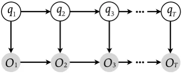
Figure 2.3: Graphical model of a hidden Markov model (HMM). The observed sequenceO1O2· · ·OT is generated by a sequence ofThidden statesq1q2· · ·qT.

2.4.1 The forward and backward approaches in HMM

Given a hidden Markov model (HMM) with Nstates and parametersq= (A,B,p),

A = {aij}, B = {bj(vk)}, p = {pi}, state sequence q = q1:T = q1q2· · ·qT, qt 2

{si}iN=1, and observation sequenceO1:T = O1O2· · ·OT,Ot 2 {vm}_mM₌₁, as illustrated in Figure 2.3, where

aij =. P(qt+1= sj |qt =si), i,j2{1, . . . ,N} bj(vm)=. P(vm |sj), 1 j N, 1m M pi =. P(q1=si), 1i N.

(2.14)

The forward-backward algorithms solve the problem of computing the likelihood of an observed sequenceO1:T, and the Viterbi algorithm and its backward variant deal

with the problem of identifying the most likely sequence of states for an observed sequenceO1:T. Interestingly, both problems can be computed either forwards or

back-wards along the observation sequence by making use of the conditional independences encoded in an HMM:

qt??q_{k2/{t 1,t}} |qt 1, 8t2 {2, . . . ,T},

qt??O1:T |qt 1, 8t2 {2, . . . ,T},

Ot??qk6=t |qt, 8t2 {1, . . . ,T}, Ot??Ok6=t|qt, 8t2 {1, . . . ,T}.

(2.15)

We first describe the forward approach of likelihood computation and sequence identification, followed by the backward approach for these two problems.

The forward algorithm

The forward algorithm is based on the insight that the likelihood of observed sequence

O1:T can be computed from the likelihood of the sub-sequenceO1:T 1, i.e.,

P(O1:T;q) =

Â

and observe that

P(O1:T,qT = si;q) =

"

Â

j

P(O1:T 1,qT 1= sj;q)·P(qT =si |qT 1 =sj)

#

·P(OT |qT = si),

(2.16)

where for simplicity, we define

P(O1:t,qt=si;q)=.

Â

P(O1:t,q1:t 1,qt =si;q).

Let at(si) =P(O1:t,qt= si;q). (2.17)

Then by Eq. (2.14) and (2.16) the likelihood ofO1:T is

P(O1:T;q) =

Â

aT(si)

=

Â

i

"

Â

j

aT 1(sj)·aji

#

bi(OT).

(2.18)

We can repeat the procedure in (2.16) to decomposeaT 1(sj), in general, we have

at(si) =

8 < :

pi·bi(Ot), t =1,

h

Âjat 1(sj)·aji

i

bi(Ot), t =2, . . . ,T.

(2.19)

Computing theat(si)values by Eq. (2.19) is known as theforward algorithm, and

the likelihood of the observated sequenceO1:T isÂiaT(si). The Viterbi algorithm

To identify the most likely sequence of states for an observed sequenceO1:T, note that

q⇤

1:T =argmax q1:T

P(O1:T,q1:T;q).

Further, similar to (2.16), we observe that the computation can be decomposed into smaller sub-problems

max

q1:T P(O1:T,q1:T;q) =maxi

⇢

max

q1:T 1 P(O1:T,q1:T 1,qT=si;q) ,

max

q1:T 1 P(O1:T,q1:T 1,qT =si;q) =maxj

⇢

max

q1:T 2 P(O1:T 1,q1:T 2,qT 1=sj;q)

·P(qT =si|qT 1=sj) ·P(OT|qT=si).

Let eat(si) =max_q

1:t 1

P(O1:t,q1:t 1,qt=si;q), (2.21)

by Eq. (2.14) and (2.20) we have

max

q1:T

P(O1:T,q1:T;q) =max

i eaT(si) =maxi

⇢

max

j eaT 1(sj)·aji bi(OT) . (2.22)

We can repeat the procedure in (2.20) to decomposeeaT 1(sj), in general, we have

eat(si) =

8 < :

pi·bi(Ot), t=1,

⇥

maxj eat 1(sj)·aji⇤bi(Ot), t=2, . . . ,T.

(2.23)

Computing theeat(si)values by Eq. (2.23) is known as theViterbi algorithm, and a

sequenceq⇤ _=q⇤

1:T with highest probability can be identified via back-tracking.

As a remark, the only difference between the forward algorithm (Eq. 2.19) and the Viterbi algorithm (Eq. 2.23) is that the former usessummationand the latter uses

maximisation(Aji and McEliece, 2000). Computations in Eq. (2.18) and (2.22) can be simplified by adding dummy (deterministic) stateqT+1 =s⇤_T+1 and observationOT+1,

P(O1:T;q) =

Â

P(O1:T+1,q1:T,qT+1=s⇤T+1;q) =aT+1(s⇤T+1) max

q1:T

P(O1:T,q1:T;q) =max_q

1:T

P(O1:T+1,q1:T,qT+1= s⇤T+1;q) =eaT+1(s⇤T+1).

The backward algorithm

Alternatively, the likelihood of an observed sequenceO1:T can be computed backwards,

note thatP(O1:T;q) =Âq1:TP(O1:T,q1:T;q), and by Eq. (2.15),

Â

q1:T

P(O1:T,q1:T;q) =

Â

Â

P(q1=si,q2:T,O1:T;q)

=

Â

i

"

Â

q2:T

P(q2:T,O2:T |q1=si;q)

#

P(q1=si)·P(O1|q1=si)

Â

q2:T

P(q2:T,O2:T |q1=si;q) =

Â

j

"

Â

q3:T

P(q3:T,O3:T |q2=sj;q)

#

P(q2=sj|q1=si)·P(O2|q2=sj)

(2.24)

Let bt(si) =

Â

qt+1:T

P(qt+1:T,Ot+1:T |qt =si;q), (2.25)

and by Eq. (2.14) and (2.24) we have

P(O1:T;q) =

Â

b1(si)·pi·bi(O1) =

Â

i

"

Â

j

b2(sj)·aij·bj(O2) #

We can repeat the procedure in (2.24) to decompose b2(sj), in general, we have

bt(si) =

8 < :

1, t= T

Âjbt+1(sj)·aij·bj(Ot+1), t= T 1 downto 1.

(2.27)

Computing the bt(si)values by Eq. (2.27) is known as thebackward algorithm, and

the likelihood of observation sequenceO1:T isÂib1(si)·pi·bi(O1).

The “backward Viterbi” algorithm

We can also identify the most likely sequence of states for observations O1:T by

computing backwards similar to (2.27), note that

max

q1:T P(O1:T,q1:T;q) =maxi maxq2:T P(q1=si,q2:T,O1:T;q)

=max i

⇢

max

q2:T P(q2:T,O2:T |q1=si;q) P(q1 =si)·P(O1 |q1=si),

(2.28) and by the conditional independences (2.15), we have

max

q2:T P(q2:T,O2:T |q1 =si;q) =maxj maxq3:T P(q2 =sj,q3:T,O2:T |q1=si;q)

=max

j

⇢

max

q3:T P(q3:T,O3:T |q2 =sj;q)

·P(q2=sj |q1=si)·P(O2|q2=sj).

(2.29)

Let

e

bt(si) =max_q t+1:T

P(qt+1:T,Ot+1:T |qt =si;q), (2.30)

by Eq. (2.14), (2.28) and (2.29) we have

max

q1:T P(O1:T,q1:T;q) =maxi

e

b1(si)·pi·bi(O1)

=max

i

⇢

max

j be2(sj)·aij·bj(O2) pi·bi(O1).

(2.31)

We can repeat the procedure in (2.29) to decompose _be₂(sj), in general, we have

e

bt(si) =

8 < :

1, t= T

maxjbet+1(sj)·aij·bj(Ot+1), t= T 1downto1.

(2.32)

q⇤

1:T with highest probability can be identified viaforward-tracking.

As a remark, the only difference between Eq. (2.27) and (2.32) is that the former usessummationand the latter usesmaximisation(Aji and McEliece, 2000). Computa-tions in Eq. (2.26) and (2.31) can also be simplified by adding dummy (deterministic) stateq0 =s⇤0 and observationO0,

P(O1:T;q) =

Â

P(O0:T,q0=s0⇤,q1:T;q) =

Â

P(O1:T,q1:T |q0=s⇤0;q) =b0(s⇤0)

max

q1:T P(O1:T,q1:T;q) =maxq1:T P(O0:T,q0=s

⇤

0,q1:T;q) =max_q

1:T P(O1:T,q1:T|q0=s

⇤

0;q) = eb0(s⇤0).

2.4.2 The list Viterbi algorithm

For tasks such as decoding digital signals corrupted by noise (e.g., speech recognition), it has been shown that considerable improvement can be obtained when a list of top

K>1 best sequences through the HMM trellis graph can be utilised (Ostendorf et al.,

1991; Seshadri and Sundberg, 1994; Nill and Sundberg, 1995; Stolcke et al., 1997). In this section, we describe algorithms that generalise the Viterbi algorithm to find the topKbest sequences from a HMM, which are known as thelist Viterbi algorithm(Nill and Sundberg, 1995; Nilsson and Goldberger, 2001).

The list Viterbi algorithm (LVA) can be employed to decode paths in a HMM by sequentially searching the next best sequence through the trellis graph until the specified number of paths are found. In Chapter 4, we make use of the LVA to deal with two challenges for path recommendations: incorporating multiple ground truths in training and eliminating loops in prediction.

Let gt(si,sj) denote the likelihood of an observed sequence O1:T such that the

states at timetandt+1 aresi andsj respectively. By Eq. (2.17) and (2.25) we have gt(si,sj) =

Â

q1:t 1,t+2:T

P(O1:T,q1:t 1,qt=si,qt+1=sj,qt+2:T;q)

=

"

Â

q1:t 1

P(O1:t,q1:t 1,qt=si;q)

#

P(qt+1=sj|qt=si)·P(Ot+1|qt+1=sj)

·

"

Â

qt+2:T

P(Ot+2:T,qt+2:T|qt+1=sj;q)

#

=at(si)·aij·bj(Ot+1)·bt+1(sj).

(2.33)

We note thatgt(si,sj)is themarginaljoint probability of all possible pairs of

observations-states (O1:T, q1:t 1sisjqt+2:T)given an HMM. Similar to Section 2.4.1, we can

(O1:T, q1:t 1sisjqt+2:T), by Eq. (2.15), (2.21) and (2.30) we have

e

gt(si,sj) =_qmax

1:t 1,t+2:TP(O1:T,q1:t 1,qt=si,qt+1 =sj,qt+2:T;q)

=

⇢

max

q1:t 1P(O1:t,q1:t 1,qt =si;q) P(qt+1 =sj |qt=si)·P(Ot+1|qt+1= sj)

· ⇢

max

qt+2:TP(Ot+2:T,qt+2:T |qt+1 =sj;q)

=eat(si)·aij·bj(Ot+1)·bet+1(sj).

(2.34) Nilsson and Goldberger (2001) proposed an algorithm to find K(K > 1) most

likely state sequences for a given observed sequenceO1:T using information encoded

inget (Eq. 2.34). It cleverly partitions the space of possible state sequences into subsets

and identifies the most likely state sequence in each subset, this procedure is repeated until allKmost likely state sequences have been found.

Algorithm 3 shows the pseudocode of the method of Nilsson and Goldberger (2001), it uses a max-heap to keep track of the sequence with the highest probability in each subset (Line 5, 7, and 14). For a sequence with the highest probability (in a subset), the algorithm maintains a partition index (i.e., the time instant at which the sequence diverges from the previous best sequence, Line 9) and an excluding set (i.e., a set of states that should be excluded at the time instant indicated by the partition index when computing the most likely state sequence in the partitioned subset, Line 11). A property ofge(Nilsson and Goldberger, 2001, Theorem 1) has been employed

to efficiently compute the probability of the most likely state sequence in a subset as well as to identify the state sequence itself (Line 12 to Line 13).

Comparison of LVA variants

We compare three typical variants of the LVA (i.e., parallel LVA, serial LVA and Algorithm 3) in terms of their time and space complexity.

The parallel LVA(Seshadri and Sundberg, 1994) finds theK best state sequences simultaneously by computing theK best state sequences in each state at each time instant. The idea is caching all the K best scores (i.e., probabilities) at each time instant instead of the best score as that in the Viterbi algorithm. This needs to find theK best scores among the NKaccumulated scores at each state and at each time instant (Seshadri and Sundberg, 1994, Eq. 6), which can be achieved by sorting the

NKaccumulated scores in timeO(NKlog(NK), or using an order statistics selection algorithm (Cormen et al., 2009, Chapter 9) with time complexityO(K_·NK). Since

Algorithm 3 The Nilsson and Goldberger (2001) list Viterbi algorithm

1: Input: HMM parametersq, observationsO_1:T, sequence lengthT,

the number of most likely sequencesK.

2: Initialise max-heapH, result setR=∆, k=1.

3: Computeeat(si)(Eq. 2.21),bet(si)(Eq. 2.30) andget(si,sj)(Eq. 2.34).

4: Identify a sequence with the highest probability (Eq. 2.23) via back-tracking: let q[1] _{= (q}[1]

1 , . . . ,q [1]

T )be the sequence andr[1] be the corresponding probability. 5: H.push(r[1]_{, (q}[1]_,nil,∆))

6: whileH₆=∆andk_ Kdo 7: r[k], (q[k],I,S) =H.pop()

Extract a state sequence with thek-th highest probability from the max-heap

H: r[k] _{is the probability ofq}[k] _{= (q}[k]

1 , . . . ,q[Tk]), I is the partition index, andSis

the excluding set.

8: Addq[k] _{to the result set R.}

9: I0 =

8 < :

1, I =nil

I, otherwise

10: fort= I0toTdo

11: S0 =

8 < :

S_[{q[k]

t }, t = I0

{q[_tk]}, otherwise

12: q_t0 =

8 > > > > < > > > > :

q[_tk0], t0 =1tot 1 argmax

s2/S0

n e

gt 1,t(q[tk]1,s) o

, t0 _=t argmax

s {get0 1,t0(qt0 1,s)}, t

0 _=t+1toT

13: r =r[k]· get 1,t(q [k]

t 1,qt) e

gt 1,t(q_t[k]₁,q[tk])

(Nilsson and Goldberger, 2001, Theorem 1)

14: H.push(r,(q,t,S0))

15: end for 16: k =k+1

17: end while

18: return result setR

O(N2KTlog(NK))orO(N2K2T). To analyse the space complexity, note that we need

O(NKT)space to store all sequence states, andO(NK)space for theNKaccumulated scores at a time instant. Therefore, the space complexity of parallel LVA isO(NKT).

globally first best sequence at a later time instant and never diverges again, since any subsequent divergence will result in a higher cost (lower score) sequence. Similarly, the third globally best sequence is either the locally third best sequence with respect to the globally first best sequence (i.e., excluding the globally second best sequence) or the locally second best sequences with respect to the globally second best sequence. This reasoning can be generalised to find theK-th best state sequence given the first, second, . . . ,(K 1)-th best state sequences.

To analyse the time complexity of the serial LVA, note that

• computing the globally best sequence using the Viterbi algorithm in time(N2T),

i.e., filling in a table with NTcells where each can be computed inO(N)time.

• computing the locally second best sequences after identifying the globallyk-th

(k= 1, . . . ,K 1)best sequences. This requires Nadditions and comparisons

in (Seshadri and Sundberg, 1994, Eq. 9) for each time instant t 2 {1, . . . ,T}, which can be upper bounded by O(NT). Thus, for all K best sequences, the time complexity isO(NKT).

• Suppose we use a priority queue to keep track of the locally best sequences, the additional cost related to insertionandextracting best operations can be upper bounded byO(KTlog(KT)). In other words, the total number of sequences in

the priority queue isKT at most, and the time for each insertion or extraction can be upper bounded by log(KT).4

Adding up these terms, the time complexity of the serial LVA is O(N2T+NKT+

KTlog(KT)), and the space complexity isW(NT+KT+NTK)i.e., the path matrix

and the “merge” count array (Seshadri and Sundberg, 1994, Eq. 9).

The analysis of the time complexity of Algorithm 3 is similar to that of the serial LVA. First, the cost of the Viterbi and “backward Viterbi” algorithms isO(N2T), then

the partitioning operations and the computation of the best sequence in each partition costO(K·NT). Lastly, the insertion and extraction of sequences costO(KTlog(KT))

if we use a priority queue. This results inO(N2T+NKT+KTlog(KT)). The space

complexity of Algorithm 3 is

O(NT+KT_·(1+T+1+N)) =O(KT2+NKT).

As a remark, the parallel LVA needs to specify the value ofKas an input of the algorithm, however, in practice, we usually do not know the value ofKbeforehand.

4_{A tighter bound isO}⇣_ÂK

k=1log(kT)

⌘