Active-set prediction for interior point methods using controlled perturbations

perturbations

.

White Rose Research Online URL for this paper:

http://eprints.whiterose.ac.uk/96569/

Article:

Cartis, C. and Yan, Y. (2016) Active-set prediction for interior point methods using

controlled perturbations. Computational Optimization and Applications, 63 (3). pp.

639-684. ISSN 0926-6003

https://doi.org/10.1007/s10589-015-9791-z

[email protected] https://eprints.whiterose.ac.uk/

Reuse

Unless indicated otherwise, fulltext items are protected by copyright with all rights reserved. The copyright exception in section 29 of the Copyright, Designs and Patents Act 1988 allows the making of a single copy solely for the purpose of non-commercial research or private study within the limits of fair dealing. The publisher or other rights-holder may allow further reproduction and re-use of this version - refer to the White Rose Research Online record for this item. Where records identify the publisher as the copyright holder, users can verify any specific terms of use on the publisher’s website.

Takedown

If you consider content in White Rose Research Online to be in breach of UK law, please notify us by

(will be inserted by the editor)

Active-set prediction for interior point methods using

controlled perturbations

Coralia Cartis · Yiming Yan

Received: date / Accepted: date

Abstract We propose the use of controlled perturbations to address the challeng-ing question of optimal active-set prediction for interior point methods. Namely, in the context of linear programming, we consider perturbing the inequality con-straints/bounds so as to enlarge the feasible set. We show that if the perturbations are chosen appropriately, the solution of the original problem lies on or close to the central path of the perturbed problem. We also find that a primal-dual path-following algorithm applied to the perturbed problem is able to accurately predict the optimal active set of the original problem when the duality gap for the per-turbed problem is not too small; furthermore, depending on problem conditioning, this prediction can happen sooner than predicting the active set for the perturbed problem or when the original one is solved. Encouraging preliminary numerical experience is reported when comparing activity prediction for the perturbed and unperturbed problem formulations.

Keywords Active-set prediction·Interior point methods·Linear programming

1 Introduction

Optimal active-set prediction — namely, identifying the active inequality con-straints at the solution of a constrained optimization problem — plays an im-portant role in the optimization process by removing the difficult combinatorial aspect of the problem and reducing it to an equality-constrained one that is in

Coralia Cartis

Mathematical Institute, University of Oxford, Andrew Wiles Building, Radcliffe Observatory Quarter, Woodstock Road, Oxford, OX2 6GG, United Kingdom.

E-mail: [email protected]

Yiming Yan

School of Mathematics, University of Edinburgh, James Clerk Maxwell Building, The King’s Buildings, Mayfield Road, Edinburgh, EH9 3JZ, United Kingdom.

E-mail: [email protected]

general easier to solve. Active-set prediction is also crucial for efficient warmstart-ing and re-optimization capabilities of algorithms when a suite of closely related problems needs to be solved. Despite being state-of-the-art tools for solving large-scale Linear Programming (lp) problems [40], Interior Point Methods (ipms) are well-known to encounter difficulties with active-set prediction due essentially to their construction. They generate iterates that progress towards the solution set through the (relative) interior of the feasible set, and thus avoid visiting possibly-many feasible vertices. This however, may also preventipms from getting accurate information about the optimal active set early enough during their running. When this information is more readily predictable/available towards the end of a run, as the iterates approach the solution set, the algorithm has to solve increasingly ill-conditioned and hence difficult, subproblems. Finding ways to improve (even just partial) active set prediction foripms could thus be beneficial as it would allow earlier termination of an otherwise ill-conditioned and computationally expensive process by say, projecting onto the solution set (as in finite termination [42]), help with reducing the problem size or with obtaining a vertex solution at the cost of just a few additional (and less expensive) simplex method iterations.

Various ways have been devised for ipms to predict the optimal active set during their run, with the simplest being cut-off [17, 23, 25] — which splits the variables into active or inactive based on whether they are less than a user-defined small value — and the most well-known beingindicators[9] which form functions of iterates and identify the optimal active-set based on whether the values of these functions are less than a threshold. Mehrotra [26] suggests determining the active set by a simple comparison of the relative increments of primal and dual iterates, and Mehrotra and Ye [28] propose a strategy to identify the active set by comparing the primal variables with the dual slacks; see [39] for a review of active-set prediction techniques for ipms for lp and also [32] for a more recent survey.

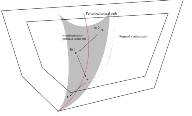
Here we propose the use ofcontrolled perturbations[5] for active-set prediction for ipms.1 Namely, we perturb the inequality constraints of the lp problem (by a small amount) so as to enlarge the feasible set of the problem, then solve the resulting perturbed problem(s) using a path-followingipmwhile predicting on the way the active set of the originallpproblem. As Figure 1 illustrates, provided the perturbations are chosen judiciously, the central path of the perturbed problem may pass close to the optimal solution of the originallpproblem when the barrier parameter for the perturbed problem is ‘not too small’. Thus we expect that while still ‘far’ from optimality for the perturbed problem, some IPM iterates for the perturbed problem would nonetheless be close to optimality for the original lp problem (such as the third and fourth iterate in Figure 1) and would provide a good prediction of the original optimal active set. As it may happen that the chosen perturbations are ‘too large’ or not sufficiently effective for active-set prediction,

1_{Note that [5] proposed the use of such perturbations for creating a sequence of LPs with}

we allow them to shrink after each IPM iteration so that the resulting perturbed feasible set is smaller but still contains the feasible set of the originallp.

Since we employ perturbed problems, albeit artificially, our proposal may be remindful of warmstarting techniques foripms and the related active-set predic-tion techniques that have been developed in that context; see for example, the surveys [11, 37]. Thus we briefly review relevant contributions here. One of the main warmstarting strategies focuses on the ‘iterates’, namely it manipulates the (ipm-computed) near optimal or optimal iterates of the initial problem to obtain a primal-dual feasible and well-centred point for the perturbed problems, see for example, [18, 21, 44, 20, 37]. Another category of approaches works on the ‘problem formulation’, namely modify the problem formulation by relaxing the nonnegativ-ity constraints in the form of shifted logarithmic barrier variables, which has some similarity to our approach. Earlier works in this framework include Freund [14, 15, 16], Mitchell [29] and Polyak [34] with promising theoretical properties. More relevant and closer in spirit to our approach here is [3], where Benson and Shanno propose a primal-dual penalty strategy relaxing the nonnegativity constraints for both primal and dual decision variables and then penalising the relaxation vari-ables in the objective; encouraging numerical results are also reported. Engau, Anjos and Vannelli [10, 11] apply a simplified primal-dual slack approach: instead of shifting the bounds and penalising the relaxation variables, slack variables for nonnegative constraints are introduced and penalised in the objective. One of the main differences between the above techniques and our approach is that we con-sider perturbations as parameters, not variables that are updated in the run of the ipm; furthermore, our focus is different as we specifically aim to predict the active set of the originallpproblem by using ‘fake’ perturbations.

Another set of techniques — regularization for ipms [35, 1, 6] — is also only loosely connected to our approach. In order to improve the conditioning of the coefficient matrix arising in calculating Newton directions inipmiterations, regu-larization terms (of proximal type, weighted, and quadratic in the variables) are added to the (primal and dual) objective function. These terms result in a di-agonal perturbation of the linear KKT system of interest, improving stability of factorization procedures. Note that the effect of our perturbations on the Newton system is not the same in that no similar diagonal perturbation is obtained. This is due to our formulations having no quadratic terms in the variables in the primal-dual objective, only a quadratic term in the perturbations; and to our approach perturbing the inequality constraints of the problem and allowing negative com-ponents of the primal and dual slack variables. However, the two techniques have similar aims in that they attempt to deal with the increasing ill-conditioning that affectsipms by improved early active-set prediction (hence earlier termination and better conditioning) for our approach and by directly improving the conditioning of the linear algebra through regularization.

Fig. 1 Enlarge the feasible set and predict the original active set

2 Controlled perturbations for linear programming

Consider the following pair of primal-dual linear programming (lp) problems,

(Primal) (Dual)

min x∈Rn c

T_x

s.t. Ax=b, x_≥0,

max (y,s)∈Rm_×Rn b

T_y

s.t. ATy+s=c, s≥0,

(PD)

where A _∈ Rm×n, b _∈ Rm and c _∈ Rn with m _≤ n are problem data, and (x, y, s)_∈Rn×Rm×Rn.

We enlarge the feasible set of this (PD) problem by usingcontrolled perturba-tions [5], namely we relax the nonnegativity constraints in (PD) and consider the pair of perturbed problems,

(Primal) (Dual)

min

x∈Rn(c+λ)

T_(x+λ)

s.t. Ax=b, x≥ −λ,

max

(y,s)∈Rm_×Rn (b+Aλ)

T_y

s.t. ATy+s=c, s_{≥ −}λ,

(PDλ)

for some vector of perturbations λ_≥0. (Note that different perturbations for x and scould be used, but for simplicity, we use the same vector of perturbations for both.) It can be checked [5] that the two problems in (PDλ) are dual to each other. Note that ifλ≡0, (PDλ) coincides with (PD). We denote the set ofstrictly

feasible points of (PDλ),

Fλ0=

n (x, y, s)

Ax=b, ATy+s=c, x+λ >0, s+λ >0 o

. (1)

Writing down the first order optimality conditions (kktconditions) for (PDλ), according for example to [31, Theorem 12.1], we find that (x∗λ, y∗λ, s∗λ) is a

(primal-dual) solution for (PDλ) if and only if it satisfies the following system,

Ax=b, ATy+s=c, (X+Λ)(S+Λ)e= 0, (x+λ, s+λ)_≥0,

(2)

whereΛ= diag(λ),X= diag(x),S = diag(s) ande= [1 . . . 1]T. Again if λ_≡0 in (2), we recover the optimality conditions for (PD).

Equivalent formulation of (PDλ). Letting p = x+λ and q = s+λ, we can write (PDλ) in the equivalent form,

(Primal) (Dual)

minp cTλp s.t. Ap=bλ,

p_≥0,

max(y,q)bTλy

s.t. ATy+q=cλ, q≥0,

wherecλ =c+λ,bλ=b+Aλandλ≥0.kktconditions ensure that (p∗λ, y∗λ, q∗λ) is the (primal-dual) solution of (3) if and only if it satisfies

Ap=bλ, ATy+q=cλ, P Qe= 0, (p, q)_≥0,

(4)

whereP = diag(p) andQ= diag(q). It is easy to show that (x∗

λ, yλ∗, s∗λ) is a (PDλ) solution if and only if (p∗λ, y∗λ, q∗λ), where p∗λ = x∗λ+λ and qλ∗ = s∗λ+λ, is a solution of (3). Thus we can construct an optimal solution for (PDλ) from an optimal solution of (3) and vice versa.

The central path of (PDλ). Following [40, Chapter 2], we derive the central path equations for (PDλ) to be

Ax=b, ATy+s=c, (X+Λ)(S+Λ)e=µ e,

(x+λ, s+λ)>0,

(5)

whereµ >0 is the barrier parameter for the perturbed problem (PDλ). The central path of (PDλ) is well defined under mild assumptions, including

Assumption: Ahas full row rankm. (6)

Lemma 1 ([5, Lemma 5.1]) Let (6)hold and λ_≥0. Then the central path of the perturbed problem (PDλ)is well defined, namely, the system (5)has a unique

solution for eachµ >0, provided _F0

λ in (1) is nonempty. In particular, ifλ >0,

F0

λ is nonempty whenever (PD)has a nonempty primal-dual feasible set.

Note that if λ >0, the condition required for the existence of the perturbed central path is weaker than that for the central path of (PD). The latter re-quires (PD) to have a nonemptystrictlyfeasible set, namely, for there to be (PD) feasible points that strictly satisfy all problem inequality constraints.

3 Perturbed problems and their properties

3.1 Perfect and relaxed perturbations

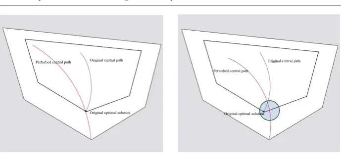
Geometrically, the original optimal solution (x∗, y∗, s∗) of (PD) may lie on or near the central path of the perturbed problem (PDλ) for carefully chosen per-turbations; see Figures 2 and 3. Algebraically, this happens if (x∗_{, y}∗_{, s}∗_{) satisfies} the third relation in (5) exactly or approximately. We make these considerations precise in the next two theorems.

Theorem 1 (Existence of ‘perfect’ perturbations) Assume (6) holds and

(x∗, y∗, s∗)is a solution of (PD). Letµ >ˆ 0. Then there exists a vector of pertur-bations

ˆ

λ= ˆλ(x∗, s∗,µˆ)>0,

such that the perturbed central path (5) with λ = ˆλ passes through (x∗, y∗, s∗)

Fig. 2 Perfect perturbations. Fig. 3 Relaxed perturbations.

Proof Since (x∗, y∗, s∗) is an optimal solution of (PD), it is also primal-dual fea-sible, and so (x∗_{, y}∗_{, s}∗_{) ∈ F}0

λ for any λ >0. Thus, according to Lemma 1, the perturbed central path is well defined. Furthermore, if there exists a ˆλ >0 such that

X∗+ ˆΛ S∗+ ˆΛe= ˆµe, (7)

then (x∗, y∗, s∗) is the unique solution of the perturbed central path equations (5) with λ = ˆλ and µ = ˆµ, which implies the central path of perturbed problems passes through (x∗, y∗, s∗). It remains to solve (7) for ˆλ = [ˆλ1 . . . λˆn]T. Since x∗is∗i = 0,i= 1, . . . , n, we have that (7) is equivalent to

ˆ

λ2i + x∗i +s∗i _ˆ

λi−µˆ= 0, i= 1, . . . , n,

whose positive root for eachigives the corresponding component of the required ˆλ.

⊓ ⊔

It is a stringent and impractical requirement to force the optimal solution of the original problem to be exactly on the central path of the perturbed problems. Thus we relax this requirement to allow for the original solution to belong to a small neighbourhood of this path.

Theorem 2 (Existence of relaxed perturbations) Assume (6) holds and

(x∗, y∗, s∗) is a (PD) solution and let µ >ˆ 0 and ξ ∈ (0,1). Then there exist vectors ˆλL = ˆλL(x∗, s∗,µ, ξˆ ) > 0 and λˆU = ˆλU(x∗, s∗,µ, ξˆ ) > 0 such that for ˆ

λL≤λ≤λˆU,(x∗, y∗, s∗)is strictly feasible for (PDλ)and satisfies

ξµeˆ _≤(X∗+Λ)(S∗+Λ)e_≤ 1

ξµe.ˆ (8)

Proof Clearly, (x∗, y∗, s∗) satisfies (1) and so (x∗, y∗, s∗)∈ F0

λfor anyλ= [λ1 . . . λn]T > 0. The inequalities (8) are equivalent to

λ2i + (x∗i +si∗)λi−ξµˆ≥0

for alli_{∈ {}1, . . . , n_}and ξ_∈(0,1). Solving (9) forλi, we obtain

   

  

λi≥ −(x∗

i+s

∗

i)+

√

(x∗

i+s∗i)2+4ξµˆ

2 =

2ξµˆ x∗

i+s∗i+ √

(x∗

i+s∗i)2+4ξµˆ

= (ˆλL)i,

0< λi≤ −(x∗

i+s

∗

i)+

q

(x∗

i+s∗i)2+

4 ˆµ ξ

2 =

2 ˆµ ξ

x∗

i+s∗i+

q

(x∗

i+s∗i)2+

4 ˆµ ξ

= (ˆλU)i,

(10)

for all i_{∈ {}1, . . . , n_}. For anyξ _∈(0,1), it is easy to see that (10) yields a well-defined interval forλi,i∈ {1, . . . , n}. ⊓⊔

From the above theorem, we see that by choosing the perturbations judiciously, we can bring any solution of the original problem into a ‘neighbourhood’ of the perturbed central path.

3.2 Preserving the optimal active set

Since we are interested in predicting the optimal active set of the original problem, this section addresses the relation between the active set of the perturbed problem and that of the originallp. We find that for sufficiently small perturbations, these two active sets remain the same provided the original problem is nondegenerate.

Theorem 3 Assume (6) holds and the original pair of (PD) problems has a unique and nondegenerate primal solutionx∗_{. Then there exists a positive scalar} ˆ

λ= ˆλ(A, b, c, x∗)such that the pair of perturbed problems (PDλ)with0≤ kλk<λˆ

has a strictly complementary solution(x∗λ, y∗λ, s∗λ)with the same active and inactive

sets asx∗, where_{k · k}denotes the Euclidean norm.

Proof Since (PD) has a unique and nondegenerate primal solution, it must have a unique primal-dual nondegenerate solution (x∗, y∗, s∗) [36, Theorem 4.5 (b)], which must be strictly complementary and sox∗+s∗>0. Thus, letting

A=i∈ {1, . . . , n}x∗i = 0 and I=

i∈ {1, . . . , n}s∗i = 0 , (11)

thekktconditions for (PD) at (x∗, y∗, s∗)—namely, (2) withλ= 0—become

x∗A= 0, x∗I>0 and s∗I= 0, s∗A>0, (12a)

AIx∗I =b, ATIy∗=cI, ATAy∗+s∗A=cA, (12b)

where A = [AI AA], (x∗)T = [(x∗A)T (xI∗)T] and (s∗)T = [ (s∗A)T (s∗I)T]. As the (PD) solution is also nondegenerate, we must have_|I|=mandrank(AI) =

m, namely, AI is nonsingular. We work with the equivalent form (3) of prob-lems (PDλ), and construct a solution (ˆp,y,ˆ qˆ) of (3) such that ˆp+ ˆq >0, ˆpA= 0 and ˆqI= 0, namely,

ˆ

pA= 0, pˆI =x∗I+λI+A−1I AAλA, (13a)

ˆ

y=y∗+ (ATI)−1λI, qˆI= 0, qˆA=s∗A+λA−(A−1I AA)TλI. (13b)

that ˆpI > 0 and ˆqA >0. Let σmax be the largest singular value of A−1_I AA, and define a positive scalar ˆλas

ˆ

λ= min{[x ∗ I s∗A]}

σmax ,

where min_{[x∗I s∗A]} is a scalar that denotes the smallest element ofx∗I and s∗A. Fromλ_≥0 and from norm properties, we have that

ˆ

pI ≥x∗I− kA−1I AAλAkeI ≥x∗I− kAI−1AAk · kλAkeI≥xI∗ − kA−1I AAk · kλkeI

and ˆ

qA≥s∗A− k A−1I AA T

λIkeA≥s∗A− k A−1I AA T

k · kλIkeA

≥s∗

A− k A−1I AA T

k · kλ_keA.

Using matrix norm properties, we obtain thatA−1_I AA

=(A−1_I AA)T

=σmax. This and 0<kλk<λˆnow imply

ˆ

pI> x∗I−σmaxˆλeI≥x∗I−min

[x∗I s∗A] eI≥0,

and

ˆ

qA> s∗A−σmaxλeˆ A≥s∗A−min

[x∗I s∗A] eA≥0,

where we also use the definition of ˆλ. _⊓⊔

Remarks on the assumptions and proof of Theorem 3.

• An equivalent non-degeneracy assumption that would be sufficient in this theorem is to require that all (PD) solutions are primal-dual nondegenerate [22, Section 5].

• We have assumed in this theorem that (PD) is primal-dual nondegenerate and has a unique solution, which guarantees AI is nonsingular. Considering the general case when (x∗, y∗, s∗) is a possibly non-unique strictly complementary solution, to construct the desired solution (ˆp,y,ˆ qˆ) of (3) with the same active set and strictly complementary partition, one needs to satisfy exactly primal-dual feasibility requirements such as

AIpˆI=b+Aλ=b+AAλA+AIλI. (14)

Clearly, one can only guarantee (14) to be consistent forλ >0 ifAAλA belongs to the range space of AI. Alternatively, one could consider satisfying (14) only approximately and look for a solution ˆpof the form

ˆ

pA= 0 and pˆI=x∗I+λI+ ˆu, (15)

4 Using perturbations to predict the original optimal active set

Recalling our main aim, we now present results for predicting the optimal active set of (PD). The idea is to solve the perturbed problem instead of the original one usingipms, but attempt to predict the active set for the original problem during the run of the algorithm. Without assuming that the original and perturbed problems have the same optimal active set, we prove that under certain conditions and given proper perturbations, when the duality gap of (PDλ) is sufficiently small, the predicted (strictly) active set for (PD) coincides with the actual optimal (strictly) active set of (PD) (Theorems 5, 6).

4.1 Some useful results

We first derive a bound on the distance between the original optimal solution set and strictly feasible points of the perturbed problems.

Lemma 2 (An error bound for(PD))Let(x, y, s)_{∈ Fλ}0, where_Fλ0 is defined in (1), andλ_≥0. Then there exists a (PD)solution(x∗_{, y}∗_{, s}∗_{)such that}

kx−x∗k ≤τp(r(x, s) +w(x, s)) and ks−s∗k ≤τd(r(x, s) +w(x, s)), (16)

whereτp>0and τd>0 are problem-dependent constants independent of(x, y, s)

and(x∗, y∗, s∗), and

r(x, s) =_kmin_{x, s_{} k} and w(x, s) =_k(₋x,₋s, xTs)+k, (17)

and wheremin_{x, s_}= ( min(xi, si) )_i=1,...,n and(x)+= ( max(xi,0) )_i=1,...,n.

See Appendix A for a proof of this lemma.

Lemma 3 [40, Lemma 5.13]For any(x, y, s)∈ F0

λ, whereFλ0 is defined in(1),

we have

0< xi+λi≤ µλ C1

(i_{∈ A}λ) and 0< si+λi ≤ µλ C1

(i_{∈ I}λ), (18)

where

µλ=

(x+λ)T_(s+λ)

n (19)

and

C1= ǫ(A, bλ, cλ)

n (20)

with

ǫ(A, bλ, cλ)

= min min i∈Iλ

sup x∗

λ∈ΩPλ

(x∗λ)i+λi , min i∈Aλ

sup (y∗

λ,s∗λ)∈ΩλD

(s∗λ)i+λi !

>0, (21)

andΩP

λ andΩDλ are the primal and dual solution sets of (PDλ)respectively, and

where (Aλ,Iλ)is the strictly complementary active and inactive partition of the

Proof Firstly, (21) is well-defined: when the feasible set of (PD) is nonempty, that of (PDλ) is also nonempty, and soǫ(A, bλ, cλ)>0. To prove the Lemma, apply [40, Lemma 5.13] to (3) and recallx=p−λands=q−λ. Note that Lemma 5.13 is a more complex result that also assumes loose proximity to the problem central path, but only strict feasibility is required to prove the required inequalities in (18). _⊓⊔

Lemma 4 Let (x, y, s)∈ F0

λ, where Fλ0 is defined in (1)for some λ≥ 0. Then

there exists a (PD) solution(x∗, y∗, s∗)and problem-dependent constants τp and τd that are independent of(x, y, s)and(x∗, y∗, s∗), such that

kx₋x∗_k< τp(C2µλ+ 4kλkmax (kλk,1))

and

ks−s∗k< τd(C2µλ+ 4kλkmax (kλk,1)),

(22)

where

C2= n

√_n

ǫ(A, bλ, cλ)+n, (23)

ǫ(A, bλ, cλ)is defined in (21)andµλ in (19).

Proof Sincex+λ >0 ands+λ >0, we have₋x < λand₋s < λ, which implies

0_≤(₋x)+< λ and 0≤(−s)+< λ. (24)

Using (19),λ≥0 and (x+λ, s+λ)≥0, we have

xTs=nµλ+λTλ−λT(x+λ)−λT(s+λ)≤nµλ+kλk2. (25)

From (17), (24) and (25), we obtain

w(x, s)≤ k(−x)+k+k(−s)+k+ (xTs)+≤nµλ+ 2kλk+kλk2. (26)

It remains to find an upper bound forr(x, s) in (17). Ifi_{∈ A}λ, from (18) we have min (xi+λi, si+λi)≤xi+λi≤ µ_Cλ

1.Similarly, we also have min (xi+λi, si+λi)≤

µλ

C1 fori∈ Iλ. Thus 0<min{x+λ, s+λ} ≤

µλ

C1e,and so from (17),

r(x, s) =kmin{x+λ, s+λ} −λk ≤ kmin{x+λ, s+λ} k+kλk ≤ µ_Cλ

1

√

n+kλk.

This, (16) and (26) now provide the bound (22). _⊓⊔

4.2 Predicting the original optimal active set using perturbations

Assume (x∗_{, y}∗_{, s}∗_{) is a (PD) solution. We denote byA(x}∗_{) the optimal active set} atx∗ and byA+(s∗), the ‘strictly’ active set ats∗, namely,

A(x∗) =i_{∈ {}1, . . . , n_{} |}x∗i = 0 and A+(s∗) =

i_{∈ {}1, . . . , n_{} |}s∗i >0 . (27) Let

¯

Theorem 4 LetC >0 and fix the perturbationλsuch that

0<kλk<min

1, C

8 max(τp, τd)

, (29)

where τp and τd are the problem-dependent constants in (22). Let (x, y, s) ∈ Fλ0

with µλ sufficiently small, namely,

µλ<

C

2C2max(τp, τd), (30)

where_Fλ0is defined in (1),µλ in (19)andC2>0in(23)is a problem-dependent

constant whenλis fixed. Then there exists a (PD)solution(x∗, y∗, s∗)such that

¯

A+(s)⊆ A+(s∗)⊆ A(x∗)⊆A¯(x).

Proof From_kλ_k<1 and (22), we have_kx₋x∗_{k ≤τ}

p(C2µλ+ 4kλk) andks−s∗k ≤ τd(C2µλ+ 4kλk), which imply

x∗i −τp(C2µλ+ 4kλk)≤xi≤x∗i +τp(C2µλ+ 4kλk) (31)

and

s∗i −τd(C2µλ+ 4kλk)≤si≤s∗i +τd(C2µλ+ 4kλk), (32) for all i ∈ {1, . . . , n}. If i ∈ A(x∗), from (29), (30) and (31), we have xi < C, namelyi_∈A¯(x). So _A(x∗)_⊆A¯(x). Ifi /_{∈ A}+(s∗),s∗i = 0. Then from (29), (30) and (32), we have si < C, namely, i /∈ A¯+(s). Thus ¯A+(s) ⊆ A+(s∗). From

x∗is∗i = 0 for alli∈ {1, . . . , n}, we haveA+(s∗)⊆ A(x∗). ⊓⊔

Theorem 4 shows that ¯_A(x) and ¯_A+(s) serve as a pair of approximations that bound_A(x∗_{). Next we go a step further and show that ¯A(x) is equivalent toA(x}∗₎ under certain conditions.

Theorem 5 Let

ψp= inf

x∗_∈ΩP_{i /∈A(}min_x∗₎(x ∗

i) (33)

whereΩP is the solution set of the primal problem in (PD) andA(x∗)is defined in (27). Assumeψp>0. Fix λandC such that

0<kλk<min

1, ψp 16 max(τp, τd)

and C = ψp

2 , (34)

whereτp andτdare the problem-dependent constants defined in(22). Let(x, y, s)∈

F0

λ with µλ sufficiently small, namely,

µλ<

ψp

4C2max(τp, τd), (35)

where _Fλ0 is defined in (1), µλ in (19) and C2 > 0 in (23). Then there exists

a (PD)solution (x∗, y∗, s∗)such that

¯

A(x) =_A(x∗),

Proof From Theorem 4 we have_A(x∗_{)⊆A¯(x). It remains to prove ¯A(x)⊆ A(x}∗_). Ifi /∈ A(x∗), from the left inequality in (31), (34) and (35), we have

xi> x∗i − ψp

2 · τp

max(τp, τd) ≥x∗inf_∈ΩP_{i /∈A(}min_x∗₎(x ∗ i)−

ψp

2 =ψp− ψp

2 =C.

Thusi /_∈A¯(x), which implies ¯_A(x)_{⊆ A}(x∗_{). ⊓⊔}

Next, we show that ¯_A+(s), the predicted strictly active set at a strictly feasible point (x, y, s) of (PDλ), is the same asA+(s∗) at some (PD) solution (x∗, y∗, s∗).

Theorem 6 Let

ψd= inf

(y∗_,s∗_)∈ΩD_i∈Amin

+(s∗)

(s∗i)

where ΩD is the solution set of the dual problem in (PD) and _A+(s∗)is defined

in (27). Assumeψd>0. Fix λandC such that

0<_kλ_k<min

1, ψd 16 max(τp, τd)

and C = ψd

2 , (36)

where τp and τd are the problem-dependent constants in (22). Let (x, y, s) ∈ Fλ0

with µλ sufficiently small, namely

µλ<

ψd

4C2max(τp, τd), (37)

where F0

λ is defined in (1), µλ in (19) and C2 > 0 in (23). Then there exists

a (PD)solution (x∗, y∗, s∗)such that

¯

A+(s) =A+(s∗),

whereA¯+(s)is defined in (28).

Proof From Theorem 4, we have ¯_A+(s) ⊆ A+(s∗). If i ∈ A+(s∗), s∗i > 0. This, (32), (36) and (37) give us

si> s∗i − ψd

2 · τd

max(τp, τd)≥(y∗_,sinf∗_)∈ΩD_i∈Amin_+(s∗₎(s ∗ i)−

ψd

2 =ψd− ψd

2 =C,

namelyA+(s∗)⊆A¯+(s). ⊓⊔

Remarks on Theorems 4–6.

• We require µλ, the mean value of the complementary products, to be suf-ficiently small in Theorems 4–6. This choice is possible since we haveµλ = 0 at any optimal solution of (PDλ) andµλ can be decreased to zero (such as in anipm framework).

•In Theorems 5 and 6, we do not require that the optimal active set of (PDλ) is the same as that of (PD) in order to be able to predict the original optimal active set of (PD).

value based on the theoretical quantityψp.) Similarly to ψp, if the dual problem in (PD) has a unique (degenerate or nondegenerate) solution, we haveψd>0.

•Fixλsufficiently small and let (xk, yk, sk) be iterates of a primal-dual path-following ipm applied to (PDλ). Then assuming these iterates belong to some good neighbourhood of the central path of (PDλ) and that the barrier parameter is decreased appropriately, we have µkλ → 0 as k → ∞ [40, Theorem 5.11]. So, by applying Theorem 5, for eachksufficiently large, there exists a (PD) solution (x∗, y∗, s∗) such that ¯_A(xk) =_A(x∗) (see also Lemma 5 below). 2

5 Comparing perturbed and unperturbed active-set predictions

5.1 Comparing with active-set prediction for (PDλ)

Consider the ‘large’ neighbourhood of the perturbed central path

N−∞(γ, λ) ={(x, y, s)∈ Fλ0|(xi+λi)(si+λi)≥γµλ, i= 1, . . . , n}, (38)

where_Fλ0is defined in (1) andµλis defined in (19); see [40, (1.16)] for the defini-tion (38) in the case ofλ_≡0.

Next we rephrase Lemma 5.13 in [40] as an active-set prediction result for (PDλ).

Lemma 5 Let(x, y, s)in_N−∞(γ, λ)andµλ defined in(19). AssumeC in(28)is

set toC= ǫ(A,bλ,cλ)γ

n , whereǫ(A, bλ, cλ)is defined in(21). Then whenµλ<µ¯ max

λ ,

where

¯ µmaxλ =

ǫ2(A, bλ, cλ)γ

n2 , (39)

for any strictly complementary solution(x∗

λ, y∗λ, s∗λ)of (PDλ)we have

¯

A(x+λ) =_A(x∗λ+λ),

where_A¯(x+λ)is defined in(28)withxreplaced byx+λand_A(x∗_λ+λ)is defined in (27)with x∗ _{replaced by x}∗

λ+λ.

Proof We work with the equivalent form (3) of (PDλ). Given (39), apply [40, Lemma 5.13] to (3), recalling thatx=p−λands=q−λ, and then we have

i_{∈ A}λ: 0< xi+λi≤ µ_Cλ

1 < C1γ≤si+λi,

i∈ Iλ: 0< si+λi ≤ _Cµλ₁ < C1γ≤xi+λi, (40)

where (_Aλ,Iλ) is the strictly complementary active and inactive partition of the solution set of (3). For any strictly complementary solution (x∗

λ, yλ∗, s∗λ) of (PDλ), (x∗λ +λ, yλ∗, s∗λ +λ) is a strictly complementary solution of (3). This and the definition ofA(x∗λ+λ) give us thatA(x∗λ+λ) =Aλ. From (40) and the definition of ¯_A(x+λ), we also have ¯_A(x+λ) =_Aλ. ⊓⊔

Substituting (23) into (35), we obtain the following threshold value

µmaxλ :=

ψpǫ(A, bλ, cλ)

4nmax(τp, τd) (√n+ǫ(A, bλ, cλ))

where ǫ(A, bλ, cλ) is defined in (21),ψp in (33), and τp and τd are the positive constants in the bounds (22). Theorem 5 provides that when ψp > 0 and λ is sufficiently small and fixed, ifµλ < µmaxλ , we can predict the optimal active set of (PD). Lemma 5 shows that whenµλ<µ¯maxλ , where ¯µmaxλ is defined in (39), we can provide the strictly complementary partition of the solution set of (PDλ) from any primal-dual pair in the neighbourhood _N−∞(γ, λ) of the perturbed central path. To verify if our approach can predict the optimal active set of (PD) before the strictly complementary partition of (PDλ), we determine conditions under whichµmaxλ >µ¯maxλ .

Theorem 7 In the conditions of Theorem 5, let

ρ= ψp

max(τp, τd). (42)

If

ǫ(A, bλ, cλ)≤ O(√nρmin (√ρ,1)), (43)

then

µmaxλ >µ¯maxλ ,

whereǫ(A, bλ, cλ)is defined in (21), µmaxλ in (41)andµ¯maxλ in (39).

Proof Note thatµmaxλ >µ¯maxλ is equivalent to

ǫ2(A, bλ, cλ) +√nǫ(A, bλ, cλ)− ρ 4γ <0,

which is satisfied if

0< ǫ(A, bλ, cλ)≤

√

n 2√γ·

ρ

√

γ+ρ+√γ. (44)

Since γ∈(0,1) and√a+b ≤√a+√b for anyaand b nonnegative scalars, we have

ρ

√_γ+ρ+√_γ ≥ √_{ρ+ 2}ρ √_γ ≥ ₃√1_γmax ρ√_ρ,1≥

√_ρ

3√γmin (

√_ρ,1).

The result follows from (44) and the above inequalities. ⊓⊔

Theorem 7 implies that when solving the perturbed problems (PDλ), ifǫ(A, bλ, cλ) is sufficiently small, we can predict the optimal active set of (PD) beforeµλ gets so small that we can even obtain the strictly complementary partition of (PDλ). To see an example when (43) is satisfied, see our remarks after Theorem 8.

Remark. In Theorem 7, we do not require the optimal active set of (PDλ) to be the same as the optimal active set of (PD). In fact, we will show that, in the numerical tests for the randomly generated problems (degenerate or nondegenerate), the optimal active sets of most perturbed problems are different from those of the original problems, but we can still predict sooner/better for (PD). In particular, the numerical experiments show that we are not solving (PDλ) to high accuracy and there are iterations where we can predict the active set for (PD) but we are not close to the solution set of (PDλ) or able to predict the active set of (PDλ);

5.2 Comparing with active-set prediction for (PD)

Similarly to Lemma 5, when we solve the original (PD) problems we can predict the optimal (PD) active set when the (PD) duality gap is smaller than some threshold. In this section, we intend to compare this threshold with the threshold value of µλ when we are able to predict the optimal active set of (PD) by solving (PDλ) and show that the latter could be greater than the former under certain conditions (Theorem 8).

Lemma 5.13 in [40] yields an active-set prediction result for (PD). In fact this result can be obtained by settingλ= 0 in Lemma 5, but for clarity, we restate it here.

Lemma 6 [40, Lemma 5.13] Let (x, y, s) in _N−∞(γ), where N−∞(γ) is the

neighbourhoodN−∞(γ, λ)in (38)with λ= 0, and letµas in (19)withλ= 0. Let

the cut-off valueC in (28)be set toC= ǫ(A,b,c_n )γ, where

ǫ(A, b, c) = min min i∈I_x∗sup_∈ΩP

x∗i, min

i∈A_(y∗_,ssup∗_)∈ΩD

s∗i !

>0, (45)

ΩP and ΩD are the primal and dual solution sets of (PD) respectively, and

(_A,_I) is the strictly complementary active and inactive partition of the solution set of (PD). Whenµ < µmax, where

µmax= ǫ

2_{(A, b, c)}

n2 γ, (46)

then for any strictly complementary solution(x∗, y∗, s∗)of (PD) we have

¯

A(x) =_A(x∗),

where_A¯(x)is defined in (28) and_A(x∗)is defined in (27).

Before we deduce a relationship between µmaxλ in (41) and µmax in (46), we first relate two other important quantities,ǫ(A, bλ, cλ) andǫ(A, b, c).

Lemma 7 Assume (6)holds and (PD)has a unique and nondegenerate solution

(x∗, y∗, s∗). Then there exists a sufficiently smallλ¯(A, b, c, x∗, s∗)>0 such that

ǫ(A, bλ, cλ)> ǫ(A, b, c) (47)

for all λsuch that 0 ≤ λ= αλ <¯ ¯λ, where α ∈(0,1), and where ǫ(A, bλ, cλ) is

defined in (21)and ǫ(A, b, c)in (45).

The proof of this lemma is given in Appendix B.

Theorem 8 In the conditions of Theorem 5, assume (6)holds and (PD) has a unique and nondegenerate solution (x∗, y∗, s∗). Provided

ǫ(A, b, c)≤ O(√nρmin (√ρ,1)), (48)

where ρ is defined in (42), there exists a sufficiently small ¯λ(A, b, c, x∗_{, s}∗_{) > 0}

such that

µmaxλ > µmax,

for all 0< λ= αλ <¯ ¯λ, where α_∈(0,1)and where µmax_λ is defined in (41)and

Proof Applying Theorem 7 withλ= 0 and so replacingǫ(A, bλ, cλ) withǫ(A, b, c), we deduce

µmax < ρǫ(A, b, c) 4n(√n+ǫ(A, b, c)).

From Lemma 7, we haveǫ(A, bλ, cλ)> ǫ(A, b, c). This and the definition ofµmaxλ in (41) give

ρǫ(A, b, c)

4n(√n+ǫ(A, b, c)) < µ max

λ .

⊓ ⊔

Theorem 8 implies that ifǫ(A, b, c) is sufficiently small, we may find the optimal active set of (PD) ‘sooner’ if we solve (PDλ) using a primal-dual path-following ipmthan if we solve (PD).

Remark. When (PD) has a unique solution (x∗, y∗, s∗), we have

ǫ(A, b, c) = min

min i∈I x

∗ i, min

i∈As ∗ i

≤min

i∈I x ∗ i =ψp.

Note that according to [24]τp, τd=O(1) numerically. Thus providedψp >1 orn is sufficiently large, (48) is satisfied. We illustrate this in an example next.

A simple example of predicting the optimal (PD) active set using perturbations.

To illustrate our results in this section, consider the following simple example

min x1+ 2x2 subject to x1+x2= 1, x1≥0, x2≥0, (49)

with the optimal solution x∗ = (1,0) and y∗ = 1, s∗ = (0,1). Thus (49) has a unique and primal-dual nondegenerate solution with optimal active set _A(x∗) =

{2_}, and so ψp = ǫ(A, b, c) = 1. Let the vector of perturbations be λ= α(1,5) where α = 10−2_{. The perturbed problems (PD}

λ) also have a unique solution x∗λ = (1 + 5α,−5α), y∗λ = 1 + α and s∗λ = (−α,1− α). So ǫ(A, bλ, cλ) = min (1 + 6α,1 + 4α) = 1 + 4α= 1.04.

First we verify the conditions in Theorem 5, which are needed in both The-orems 7 and 8. Since it is not clear how to deduce the value of τp and τd, we estimate them numerically2_{and it turns out thatτ}

p ≈τd ≈0.8. We set the cut-off constantC that separates the active and inactive constraints to beC= ψp

2 = 0.5 and verify that_kλ_k=√26α < ψp

16 max(τp,τd) <1. Thus the conditions in (34) are

satisfied. Based on Theorem 5, we can predict the original optimal active set when µλ is less thanµmaxλ ≈0.0662.

Next we verify Theorems 7 and 8. From (7), we getρ_≈1.25, and so√nρmin √ρ,1_≈ 1.58. Thus 0< ǫ(A, b, c)< ǫ(A, bλ, cλ)<√nρmin √ρ,1, which implies that con-ditions (43) and (48) are satisfied. For the constantγ, it is common to choose a small value to have a large neighbourhood of the central path; setγ= 0.01. Then from (39) and (46), we have ¯µmaxλ ≈0.0027< µλmax andµmax= 0.0025< µmaxλ . This implies that when we use perturbations, we can predict the original optimal

2_{We estimateτpandτ}

dfrom their definition in (16), namely, we solve the following

opti-misation problem inmatlab, maxkx−x∗_{k/(r(x, s) +w(x, s)) subject to (x, y, s)∈ F}0

λ, where

r(x, s) andw(x, s) are defined in (17) andF0

active set sooner than the perturbed active set or the original active set without perturbations. Furthermore, the threshold values (constantC) needed to separate the active constraints from the inactive ones for predicting the perturbed active set and the original active set without perturbations are 0.0052 and 0.005 respectively, both of which are much smaller than the cut-offC = ψp

2 = 0.5 for predicting the original optimal active set using perturbations.

6 Numerical results

6.1 The perturbed algorithm and its implementation

All numerical experiments in this section employ an infeasible primal-dual path-following interior point method structure [40, Chapter 6] whether applied to (PDλ) or (PD). The perturbed algorithm is summarised in Algorithm 1.

Algorithm 1: Perturbed Algorithm Framework.

Givenperturbations (λ0_{, φ}0_{)>0 and a starting point (x}0_{, y}0_{, s}0_{) with (x}0_+λ0_{, s}0_+φ0_)>

0,fork= 0,1,2, . . .

solvethe perturbed system (5) using Newton’s method, namely





A 0 0

0 AT _I

Sk_+Φk _{0 X}k_+Λk



 

 ∆xk

∆yk

∆sk



=− 



Axk_−b

AT_yk_+sk_−c

Xk_+Λk

Sk_+Φk

e−σk_µk λe



, (50)

whereσk_{∈[0,1] and}

µk λ=

(xk_+λk₎T_(sk_+φk₎

n ; (51)

setxk+1_=xk_+αk

p∆xkand (yk+1, sk+1) = (yk, sk) +αkd(∆yk, ∆sk), where

(αk

p, αkd) is chosen such that (xk+1+λk, sk+1+λk)>0;

predictthe optimal active set of (PD) and denote byAk_;

terminateif some termination criterion is satisfied;

calculate(λk+1_{, φ}k+1_{) possibly by shrinking (λ}k_{, φ}k_{) so that}

(xk+1_+λk+1_{, s}k+1_+φk+1_)>0;

end (for).

Algorithm without perturbations. For comparison purposes, we refer to the algo-rithm with no perturbations (Algoalgo-rithm 1 withλ=φ= 0) as Algorithm 2. We denote the duality gap for Algorithm 2 as µk_{, which is equivalent to µ}k

λ in (51) withλk=φk= 0.

This change did not affect our results in any significant way, suggesting some level of robustness.)

Solving the Newton system (50). We follow [40, Chapter 11] and solve the aug-mented system form of (50). Also we setσk= min(0.1,100µkλ).

Choice of perturbations. In our theory, we used the same vector of perturbations for both primal and dual variables. For better numerical efficiency, we have dif-ferent perturbations λ and φfor primal and dual variables respectively. We set the initial perturbations to beλ0_=φ0_{= 10}−2_{e, whereeis a vector of ones. (We} have done experiments to explore the sensitivity of our algorithm to the value of the initial perturbations. For example, choosing λ0 = φ0 = 10−1e yields a high false-prediction ratio (proportion of mistakes). Perturbations of order 10−2 and 10−3yield quickly a good approximation of the original (PD) active set. For λ0 =φ0 = 10−4e, the perturbed algorithm starts to behave similarly to the un-perturbed one simply because the perturbations are too small.)

Choice of stepsize. We choose a fixed, close to 1, fraction of the stepsize to the nearest constraints’ boundary in the primal and dual spaces, respectively.

Shrinking the perturbations. One possible reason for getting a poor prediction of the active set is that the current perturbations are too large. So after we get the new iterate (xk+1, yk+1, sk+1), we shrink the perturbations accordingly. Assume tk+1= min(xk+1) andvk+1= min(sk+1). We update the perturbations as follows,

λk+1= (

ηλk, iftk+1>0

(1−ζ)λk+ζ(−tk+1)e, iftk+1≤0,

and

φk+1= (

ηφk, ifvk+1>0

(1−ζ)φk+ζ(−vk+1)e, ifvk+1≤0,

whereη_∈(0,1] andζ _∈(0,1). It follows thatxk+1+λk+1>0 andsk+1+φk+1> 0. We observed in our numerical experiments that when solving nondegenerate problems, it is better to shrink faster, roughly keeping the perturbations to be

O(µλ). When solving degenerate problems however, it is better to shrink slower, at a rate of O(√µλ). It is difficult and often impossible to distinguish a priori between degenerate and nondegenerate cases. After several numerical trials, we chose to setη= 1 andζ= 0.5.

Active-set prediction. In our theory, we considered that all variables less than a threshold are active at the solution. In practice, we apply a more complex strategy, inspired by [9, Step 3 in Procedure 8.1]. We partition the index set {1,2, . . . , n}

into three sets, Ak _{as the predicted active set, I}k _{as the predicted inactive set} and _Zk = _{1,2, . . . , n_{}\ A}k_{∪ I}kwhich includes all undetermined indices, and during the running of the algorithm, we move indices between these sets according to the following criteria,

where C is a constant user-defined threshold. Theorem 4 guarantees the above criteria (52) are promising, as we are predicting the original optimal active set by estimating the intersection of ¯A+(ski) and ¯A(xki). InitialiseA0 =I0 =∅ and

Z0=_{1,2, . . . , n_}. An index is moving from_Zk to_Akif (52) is satisfied for two consecutive iterations, otherwise from _Zk to _Ik. We move an index from _Ak to

Zk_{if (52) is not satisfied at the current iteration. An index is moving fromI}k _to

Zk _{if (52) is satisfied at the current iteration. In our implementation, we choose} C = 10−5. Procedure 1 in Appendix C contains a pseudocode of our active-set prediction technique. Our strategy enables us to make use of both primal and dual information which may be beneficial given Theorems 4–6.

Termination. Termination criteria will be defined for each set of tests.

6.2 Numerical results

6.2.1 Test problems

Randomly generated test problems (TS1). We first randomly generate the number of constraintsm_∈(10,200), the number of variables n_∈(20,500) and density of nonzero entries inAwithin (0.4,0.8), wherem < n, 2m < n <7m. Then randomly generate a matrixA_∈Rm×nof given density and a point (x, y, s)_∈Rn×Rm×Rn

with x_≥ 0, s_≥ 0 and density about 0.5. Finally we generate band c by letting b = Ax and c = A⊤y +s. Thus (x, y, s) serves as a feasible point. Problems generated this way are generally well-conditioned and primal nondegenerate. This test set is inspired by the random problem generation approach in [13, Section 8.3.4].Whenever we use this test set, (the same) 100 problems are generated.

Randomly generated primal-dual degenerate test problems (TS2). Instead of gen-erating a feasible point as for TS1, we generate (x, y, s) withx≥0,s≥0,xisi= 0 for all i_{∈ {}1, . . . , n_} so that the number of nonzeros of xis strictly less than m and that ofsis strictly less thann₋m. Then getA,b,cas for TS1. Thus (x, y, s) serves as a primal-dual degenerate solution. 100 problems are also generated for this test set.

Netlib problems (TS3). Most Netlib test problems are not in the standard form. We reformulate them into the standard form by introducing slacks. Since our implementation is basic, inmatlab, and mainly for illustration, we choose a subset of problems in Netlib with the number of primal variables less than 5000 (including the slack variables). See Table 3 for the list of the 37 Netlib problems selected.

6.2.2 On the accuracy of active-set predictions using prediction ratios

AssumeAk _{is the predicted active set at iterationkand Ais the actual optimal} active set. To compare the accuracy of the predictions, we introduce the following three prediction ratios.

– Missed-prediction ratio = |A \_|A(Ak_{∪ A|}k∩ A)|.

– Correction ratio = |A_|Akk∩ A|_{∪ A|}.

False-prediction ratio measures the degree of incorrectly identified active con-straints, missed-prediction ratio measures the degree of incorrectly rejected active constraints and correction ratio shows the accuracy of the prediction. All three ratios range from 0 to 1. If the predicted set is the same as the actual optimal active set, correction ratio is 1. The main task for this test is to compare the three measures for Algorithms 1 and 2.

When anlpproblem has multiple solutions, the active set of a vertex solution is different from that of the strictly complementary solutions (about 17% difference on average for TS1 and 21% for TS2). To understand which active set do the (perturbed) Algorithm 1 and the (unperturbed) 2 predict, we terminate both algorithms at the same iteration and compare the predicted active sets with the actual optimal active sets obtained from an interior point solver and a simplex solver3.

Prediction ratios for test sets TS1 and TS2. In Figures 4 and 5, we present the results for TS1 (left) and TS2 (right). The x-axis shows the number of interior point iterations at which we terminate the algorithms. In each figure, the first three plots (from left to right, top to bottom) show the average value of the three measures mentioned above for the test problems in question. The last plot at the bottom right corner presents the corresponding log₁₀scaled relativekktresiduals. We measure the relative residual by

relResk= || Ax

k_{−b, A}T_yk_+sk_{−c, X}k_+Λk _Sk_+Φk_e−µk λe

||

1 + max (_||b_||,_||c_||) . (53)

There are four lines in each plot, representing the prediction ratios by comparing the active set from Algorithm 1 with that frommatlab’s simplex solver (solid red line with circle) and frommatlab’s ipm(solid black line with square sign), and Algorithm 2 with simplex (dashed green line with diamond sign) and with ipm (dashed blue line with star) respectively.

– Figures 4 and 5 show that the average correction ratios for Algorithm 1 are at least as good and generally better than those for Algorithm 2. Thus it seems that using perturbations can only improve the active-set prediction capabilities ofipms.

– Algorithm 2 is in fact an interior point solver applied to (PD) which approaches a strictly complementary (PD) solution. This is confirmed by having better cor-rection ratio when comparing Algorithm 2 with theipmthan when comparing it with the simplex.

– Due to the fact that the active set from the ipm(the strictly complementary partition) contains less elements than that from the simplex (vertex solution), the correction ratio of Algorithm 1 compared with theipmis higher than that compared with the simplex at the early stage. However the false-prediction

3 _{We obtain the ‘actual optimal active set’ by solving the problem usingmatlab’s solver}

6789 10 11 12 13 14 15 16 17 18 0 0.2 0.4 0.6 0.8 1

False Prediction Ratio

6789 10 11 12 13 14 15 16 17 18 0 0.2 0.4 0.6 0.8 1

Missed Prediction Ratio

6789 10 11 12 13 14 15 16 17 18 0 0.2 0.4 0.6 0.8 1 Correction Ratio

6789 10 11 12 13 14 15 16 17 18 −7 −6 −5 −4 −3 −2

Average Relative Residual (log10)

Alg 6.1 − Splx Alg 6.1 − IPM Alg 6.2 − Splx Alg 6.2 − IPM

Fig. 4 Prediction ratios for randomly

generated problems

6789 10 11 12 13 14 15 16 17 18 0 0.2 0.4 0.6 0.8 1

False Prediction Ratio

6789 10 11 12 13 14 15 16 17 18 0 0.2 0.4 0.6 0.8 1

Missed Prediction Ratio

6789 10 11 12 13 14 15 16 17 18 0 0.2 0.4 0.6 0.8 1 Correction Ratio

6789 10 11 12 13 14 15 16 17 18 −7 −6 −5 −4 −3 −2

Average Relative Residual (log10)

Alg 6.1 − Splx Alg 6.1 − IPM Alg 6.2 − Splx Alg 6.2 − IPM

Fig. 5 Prediction ratios for randomly

generated primal-dual degenerate

ratios of the former climb up to about 0.16 at the end for both test cases. Thus the corresponding correction ratios go down. The false-prediction ratios of comparing Algorithm 1 with simplex are much less, about 0.05 for both cases. The behaviours of the false-prediction ratios seem to imply that Algorithm 1 predicts the active set of a vertex solution (that may not be the same vertex as obtained by the simplex solver).

– After 18 iterations, the correction ratios do not reach 1. This is due to ill-conditioning which prevents us from solving any further. For this 18th_iteration, the perturbations are not zero, they are about O(10−2) for problems in TS1 and O(10−3) for the degenerate problems in TS2, and on average the relative residual (53) is lower than 10−6.

Can Algorithm 1 predict the optimal active set of (PD)sooner than it obtains the strictly complementary partition of (PDλ)? In Figures 6 and 7, besides compar-ing the predicted active set of (PD) with the actual active set of (PD), we also compared the predicted active set of (PDλ)4 with the actual active set of (PDλ) obtained from a simplex solver (solid purple line with downward-pointing triangle) and anipmsolver (dashed brown line with upward-pointing triangle), respectively; see Footnote 3 on the choice of solvers. We again use the test sets TS1 and TS2.

We can see that on average Algorithm 1 can predict a better active set for (PD) than when applying Algorithm 2 to predict the active set of (PDλ). Furthermore, for test case TS1, before iteration 12, Algorithm 2 cannot predict much concerning the active set of (PDλ) while Algorithm 1 already has an increasingly accurate prediction for the active set of (PD) (approximately 80% of the active set of (PD) at iterations 12). We can draw similar conclusions for TS2.

On the difference between the optimal active set of (PDλ) and that of (PD). Note that, to yield good performance, we do not need to force the active set

4 _{Here, for each of the test problems, we setλ in (PD}

λ) to be the value of the

pertur-bations when terminating Algorithm 1 at the 18th _{iteration. We then apply Algorithm 2 to}

the equivalent form (3) of (PDλ), which means we solve the perturbed problem using anipm

6789 10 11 12 13 14 15 16 17 18 0 0.2 0.4 0.6 0.8 1

False Prediction Ratio

6789 10 11 12 13 14 15 16 17 18 0 0.2 0.4 0.6 0.8 1

Missed Prediction Ratio

6789 10 11 12 13 14 15 16 17 18 0 0.2 0.4 0.6 0.8 1 Correction Ratio

6789 10 11 12 13 14 15 16 17 18 −7 −6 −5 −4 −3 −2

Average Relative Residual (log10)

Alg 6.1 − Splx Alg 6.1 − IPM Alg 6.2_P − Splx_P Alg 6.2_P − IPM_P

Fig. 6 Comparing perturbed active-set

predictions for (TS1)

6789 10 11 12 13 14 15 16 17 18 0 0.2 0.4 0.6 0.8 1

False Prediction Ratio

6789 10 11 12 13 14 15 16 17 18 0 0.2 0.4 0.6 0.8 1

Missed Prediction Ratio

6789 10 11 12 13 14 15 16 17 18 0 0.2 0.4 0.6 0.8 1 Correction Ratio

6789 10 11 12 13 14 15 16 17 18 −7 −6 −5 −4 −3 −2

Average Relative Residual (log10)

Alg 6.1 − Splx Alg 6.1 − IPM Alg 6.2_P − Splx_P Alg 6.2_P − IPM_P

Fig. 7 Comparing perturbed active-set

predictions for (TS2)

of (PDλ) (as defined in Footnote 4) to be the same as the (original) active set of (PD). In fact, for most test problems in both TS1 and TS2, this does not hold. When perturbations are not so small, namely O(10−2) or O(10−3), which is the case even in the last ipm iterations in Figures 6 and 7, the perturbed optimal active set is different from the original optimal active set for 98% of the test problems in TS1 and all test problems in TS2. Furthermore, for problems in TS1, the average difference between the strictly complementary partition of (PDλ) and that of (PD) is as high as 33% and the difference between the active set at a vertex solution of (PDλ) and that of (PD) is about 15% on average; for TS2, the average difference between the strictly complementary partitions of (PDλ) and (PD) is about 29% and the difference between active sets at vertex solutions is 17% on average. Another interesting observation is that, for both TS1 and TS2, over 90% of the perturbed problems have a unique and nondegenerate solution, regardless of the uniqueness or degeneracy of the original test problems. This is the reason why the predictions of the perturbed active set when comparing with simplex and ipmare identical in Figures 6 and 7.

matlab’s simplex solver (solid red line with circle) and frommatlab’sipm(solid black line with square sign), and Algorithm 2 with simplex (dashed green line with diamond sign) and withipm(dashed blue line with star), respectively. The bottom right figure plots the corresponding average relative residual (53) on a log₁₀scale.

M-9 M-8 M-7 M-6 M-5 M-4 M-3 M-2 M-1M 0

0.2 0.4 0.6 0.8 1

False Prediction Ratio

M-9 M-8 M-7 M-6 M-5 M-4 M-3 M-2 M-1M 0

0.2 0.4 0.6 0.8 1

Missed Prediction Ratio

M-9 M-8 M-7 M-6 M-5 M-4 M-3 M-2 M-1M 0

0.2 0.4 0.6 0.8 1

Correction Ratio

M-9 M-8 M-7 M-6 M-5 M-4 M-3 M-2 M-1M -10

-9 -8 -7 -6 -5 -4 -3 -2 -1

0 Average Relative Residual (log10)

Alg 6.1 - Splx Alg 6.1 - IPM Alg 6.2 - Splx Alg 6.2 - IPM

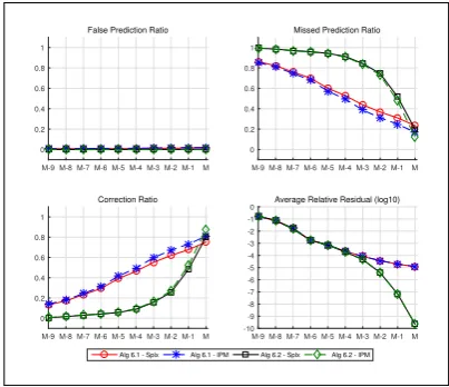
Fig. 8 Comparing prediction ratios for the Netlib problems in TS3.Mdenotes the (variable)

total number of iterations required to solve each test problem to a given accuracy (thusM is generally different for each test problem).

– Figure 8 shows that using perturbations can only improve the active-set predic-tion capabilities ofipms on the tested Netlib problems, especially in the earlier stages of the runs, when the relative residuals are not too small. For example, the average correction ratios when using Algorithm 1 are about three times better than those of using Algorithm 2 at iteration M−5, when the average relative residual is just slightly less than 10−3.

– The correction ratios for both algorithms are slightly worse when compared with the vertex solution frommatlab’s simplex solver than with the strictly complementary solution from matlab’sipm solver; thus it is unclear in this case whether Algorithm 1 gets us closer to a vertex or an interior solution of the original problem (the cross-over to simplex results for TS3 in the next section seem to indicate the former is still the case).

– The average relative residual in the bottom right plot is still quite large over the last few iterations for Algorithm 1 indicating that we have not solved the perturbed problems to high accuracy while still being able to predict well the optimal active set of the original problem, as desired.

6.2.3 Crossover to simplex

lp solve [4] as our simplex solver (as its matlabinterface allows us to set the initial basis).

Initial basis for the simplex method. Assume we terminate the perturbed algorithm Algorithm 1 at the kth iteration, with the predicted active set _Ak. To generate an initial basis_Bfrom_Ak, we first obtain all independent columns inAIk. If this

submatrix is not of rankm, we choose a column from AAk and append it to the

submatrix provided it is independent of existing columns in the submatrix. The order in which columns are added back in is decided by dual information, namely we keep trying a series of columns _{Ait}, where it ∈ A

k _{and s}k i1 ≤ s

k

i2 ≤ . . .≤

ski_|Ak|, until a full rank square matrix is obtained. Since Ais full row rank 5_{, this} procedure is finite. A similar approach has been used in [38, Section 7] to form a basis ofA.

To conduct the tests, we first choose a thresholdµcap_λ , run Algorithm 1, termi-nate the algorithm whenµk

λ< µcapλ , record the number of interior point iterations, sayK, generate an initial basisBby the above procedure and finally start the sim-plex solverlp solvefrom the initial basisB. For comparison purposes we perform exactlyKiterations of Algorithm 2, and generate a new basis for (PD) by the same procedure, without constraining the value ofµk. All tests in this part are run with µcap_λ = 10−3_.

We compare the number of simplex iterations used to get an optimal solution after crossover from Algorithms 1 and 2, visualising the results via a relative performance profile [30]. Namely, we consider the following relative iteration count,

rli=−log2 Iterp_i Iter0 i

, (54)

whereistands for theithproblem, the numerator stands for the number of simplex iterations performed after Algorithm 1 and the denominator measures the same but after Algorithm 2. If, for problemi, Algorithm 1 uses fewer simplex iterations, we get a positive valued bar with height = rli. If Algorithm 2 wins, we obtain a negative valued bar with height defined as₋rli. The value of the bar will be 0 if these two yield the same simplex iterations orlp solvefails for both algorithms. Iflp solvefails to solve problemifor Algorithm 1, we have a negative valued bar with height of maxi(|rli|), otherwise a positive valued bar with the same height. It is clear that the winner outperforms the loser by 2|rli| _{times and one algorithm}

outperforms the other by having more bars (or larger area of bars) in its direction.

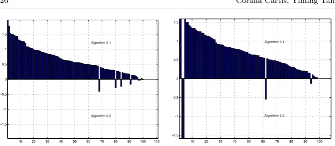
Crossover to simplex for randomly generated test problems (TS1 and TS2). In Figures 9 and 10, we show the profiles for TS1 (left) and TS2 (right), with bars sorted from largest to smallest in height. We can see that, counting the number of simplex iterations after each algorithm, the performance of Algorithm 1 dominates that of Algorithm 2 in both cases.

In Table 1, we show the average number of simplex iterations, the average ipmiterations and the averageµkλ andµkwhen we terminate Algorithms 1 and 2 for both test sets (TS1 and TS2). On average, using perturbations saves about

5_{In our tests, we apply the preprocessing code fromlipsol[45] to ensure thatAis full row}

10 20 30 40 50 60 70 80 90 100 110 −1.5

−1 −0.5 0 0.5 1 1.5

Algorithm 6.1

Algorithm 6.2

Fig. 9 Simplex iteration count for randomly

generated problems

10 20 30 40 50 60 70 80 90 100 −1.5

−1 −0.5 0 0.5 1 1.5

Algorithm 6.1

Algorithm 6.2

Fig. 10 Simplex iteration count for

ran-domly generated primal-dual degenerate problems

34% simplex iterations for the test case TS1 and about 37% for TS2. Due to our experimental setup, the number of ipmiterations are the same for Algorithms 1 and 2, and the average finalµk_λ andµkbefore crossover are of order 10−4.6

Table 1 Crossover to simplex whenµk

λ<10−3 for random problems.

Primal nondegenerate (TS1) PD degenerate (TS2) Algorithm 1 Algorithm 2 Algorithm 1 Algorithm 2

Avg simplex iterations 287 436 292 464

Avgipmiterations 10 10 10 10

Avgµk

λandµkwhen crossover 7.33×10−4 6.80×10−4 7.53×10−4 7.14×10−4

We also tracked the difference between the initial bases generated from Algo-rithms 1 and 2. We use relative difference7 to measure the degree of difference between two bases. On average the relative difference is over 60%, and over 90% of the test problems have greater than 50% relative difference. Thus our preliminary numerical experiments illustrate that using perturbations is likely to improve the efficiency when crossing over to simplex.

Netlib test problems (TS3). The good prediction performance of the perturbed algorithm is not only obtained for randomly generated problems, but also for the subset of Netlib problems (TS3). Here we add an additional termination criterion, namely we terminate both algorithms whenµk_λandµkare less than 10−3or when the relative residual (53) is less than 10−6_{, whichever occurs first}8_.

6_{The definition ofµ}k

λandµkin Algorithms 1 and 2, respectively, as well as the choice of

(x0_{, s}0_{) to be identical for (PD}

λ) and (PD), imply thatµ0λ> µ0, with the difference being

essentially dictated by the level of perturbations (λ0_{, φ}0_{). Thus we are not making it any easier}

for Algorithm 1 compared to Algorithm 2 in the choice of starting point.

7_{The number of elements in either basis generated from Algorithms 1 or 2 but not both}

divided by the cardinality of the union of two bases.

8_{This is because some problems have very large components in the right hand sidebwith}

max(b)>103_{. For these problems, even whenµ}k

λ>10−3, the relative residual may already be

less than 10−6_{and this causes numerical problems when trying to decreaseµ}k

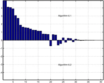
Figure 11 presents the relative performance profile generated the same way as for the random tests (see (54) and accompanying explanation). From this fig-ure, we can see that for over half of the test problems, Algorithm 1 outperforms Algorithm 2 by over 1.5 times. Algorithm 1 ‘loses’ for only 7 problems.

5 10 15 20 25 30 35 40

−4 −3 −2 −1 0 1 2 3 4

Algorithm 6.1

Algorithm 6.2

Fig. 11 Crossover to simplex for 37 Netlib problems

We also summarise the results in Table 2. On average, we save about 38% simplex iterations by applying perturbations. The average numbers in the table exclude the data forship08s, sincelp solvefails to solve it when we do not apply perturbations.

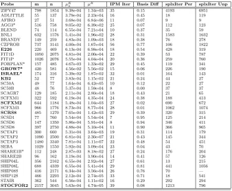
Table 2 Crossover to simplex whenµk

λ<10−3 for 37 Netlib problems (TS3).

Algorithm 1 Algorithm 2 Avg simplex iterations 358 612

Avgipmiterations 22 22

We do not give the average value ofµkλin the table as it is more involved than for random problems. In particular, for the problems with very large component in b (problems marked by * in Table 3 ), the value of µkλ is greater than 10−3 for both Algorithms 1 and 2. There are 8 additional problems, including25fv47, bnl1, brandy, kb2, scfxm2, scrs8, scatp1 and stair, for which the value of µkλ is less than 10−3only when we apply perturbations. This seems to imply that using perturbations can somehow accelerate the interior point method procedure or yield better conditioning. Except for these particular problems, the average value ofµk_λ is of order 10−4. For detailed data, see Table 3.

As for randomly generated problems, we also tracked and compared the differ-ences between initial bases obtained from Algorithms 1 and 2. We use the same relative difference measure (see Footnote 7). The average difference is about 40%,

but there are 9 problems9 _{with relative difference less than 10%. Algorithm 1 is} no better than Algorithm 2 for these problems. Generally, for small problems with small relative differences between bases, the simplex iterations are quite similar; for large problems, even small relative difference can yield quite different simplex iterations (such as forsebaandstocfor2). The disappointing small relative dif-ference of initial bases may be the result of inappropriate initial perturbations, improper shrinking speed of perturbations or ill-conditioning.

7 Conclusions and future work

We have proposed the use of controlled perturbations for improving active set pre-diction capabilities of ipms for lp. The perturbations are chosen so as to slightly enlarge the feasible set in the hope that the central path of the perturbed problems passes through or close to the original solution set when the perturbed barrier pa-rameter is not too small. Our approach solves a (sequence of) perturbed problems using a standard primal-dual path-following method and predicts using cut-off, the optimal active set of the original problem on the way. We have provided theoretical and preliminary numerical evidence that this approach to active-set prediction for ipms looks promising in that the perturbed problems are not being solved to high accuracy before the original optimal active set can be accurately predicted and that the perturbations help with the accuracy and speed of the activity prediction for the original solution set.

There are several issues remaining for full validation of the proposed approach; such as the choice of the initial perturbations which we currently set to a fixed small value that we then adjust, but that may be more suitably set to some problem-dependent value. At present, we have used cut-off to predict the original optimal active set when solving the perturbed problems (PDλ); we plan to explore other suitable techniques for the prediction such as the identification function

proposed originally for nonlinear programming [12]. Note that indicators [9] are not suitable for our purposes as they can only predict the perturbed optimal active-set when calculated in the context of an ipmapplied to (PDλ). Finally, a large-scale implementation and testing of the perturbed approach and prediction is needed to complete our numerical experiments forlp. From a theoretical point of view, it would be important to show polynomial complexity of a safeguarded (say, long-step [40]) variant of Algorithm 1; this seems achievable since one can think of Algorithm 1 as a standard primal-dual path-following ipmapplied to solving (to some accuracy) a sequence of lpproblems (PDλ), and so each solve of a (PDλ) could be shown to have polynomial complexity.

There are several interesting/important areas that may benefit from the appli-cation of the controlled perturbations approach for active-set prediction foripms. For example, it may prove useful for improvingwarmstarting capabilities[11, 37] of ipms. Furthermore, it could be applied to the Homogeneous Self-Dual (hsd) em-bedding model[43, 41] for anlp, which is a very useful re-formulation that allows assessing whether the givenlpproblem has a solution, as well as finding this solu-tion, depending on whether some auxiliary variables are active or inactive at the solution of thehsdproblem. Thus early and accurate activity prediction forhsd