©2017 The Authors Journal of the Royal Statistical Society: Series C (Applied Statistics) Published by John Wiley & Sons Ltd on behalf of the Royal Statistical Society.
This is an open access article under the terms of the Creative Commons Attribution-NonCommercial-NoDerivs License, which permits use and distribution in any medium, provided the original work is properly cited, the use is non-commercial and no modifications or adaptations are made.
0035–9254/17/66997 66,Part5,pp.997–1013
The use of heuristic optimization algorithms to
facilitate maximum simulated likelihood estimation
of random parameter logit models
Arne Risa Hole
University of Sheffield, UK
and Hong Il Yoo
Durham University, UK
[Received August 2015. Final revision November 2016]
Summary.Applications of random-parameter logit models can be found in various disciplines. These models have non-concave simulated likelihood functions and the choice of starting values is therefore crucial to avoid convergence at an inferior optimum. Little guidance exists, however, on how to obtain good starting values. We apply an estimation strategy which makes joint use of heuristic global search routines and gradient-based algorithms. The central idea is to use heuristic routines to locate a starting point which is likely to be close to the global maximum, and then to use gradient-based algorithms to refine this point further. Using four empirical data sets, as well as simulated data, we find that the strategy proposed locates higher maxima than more conventional estimation strategies.
Keywords: Differential evolution; Generalized multinomial logit; Mixed logit; Particle swarm optimization
1. Introduction
With an increase in desktop computing power, the random parameter logit (RPL) model has become increasingly common in empirical applications. Also known as the mixed logit, the RPL model provides a flexible framework for modelling discrete choice data. It can approximate any random-utility maximization model arbitrarily well subject to specifying a suitable joint distri-bution of parameters (McFadden and Train, 2000) and incorporate preference heterogeneity between different individuals alongside panel correlation across observations on the same in-dividual (Revelt and Train, 1998). Applications of the RPL model can be found in a range of disciplines including economics, marketing science, transportation studies and health services research.
Although the RPL model is specified by augmenting the parameters of the multinomial logit model with random heterogeneity, it poses some estimation issues which the multinomial logit model does not. Perhaps the best known is that, in most applications, the RPL likelihood is a multi-dimensional integral which has no closed form expression and needs to be numeri-cally approximated by using simulation. This issue has motivated several studies to explore how best to obtain a more accurate approximation from a given number of draws from the
Address for correspondence: Arne Risa Hole, Department of Economics, University of Sheffield, 9 Mappin Street, Sheffield, S1 4DT, UK.
joint distribution of random parameters (Train (2009), pages 205–236), and their findings have popularized the use of Halton sequences to generate draws. Although progress has also been made on developing estimation methods which are more computationally attractive than the classical method of maximum simulated likelihood (MSL) in certain aspects (Huber and Train, 2001; Harding and Hausman, 2007; Train, 2008), MSL still remains the most commonly used method as it can be readily applied in conjunction with almost any joint distribution of random parameters.
This paper applies an estimation strategy to address another well-known estimation issue, on which limited practical guidance exists. Specifically, in contrast with its multinomial logit counterpart, the RPL likelihood is not globally concave and may feature several local maxima. As in other similar contexts of non-linear estimation, the selection of ‘good’ starting values for estimated parameters is crucial to avoid an inferior local maximum. In the RPL literature, nevertheless, empirical studies rarely provide an explicit discussion of starting values used, and the question of how to obtain good starting values has not been the subject of inquiry as far as we know.
Our proposed estimation strategy makes joint use of heuristic optimization algorithms and the usual gradient-based algorithms to obtain the MSL estimates of the RPL. Following Dorsey and Mayer (1995), the central idea is to use heuristic algorithms to locate a starting point which is likely to be close to the global maximum, and then to use gradient-based algorithms to refine this point further. For the heuristic search step, we consider two parsimonious but effective algorithms which can be easily implemented by non-specialists in heuristic optimization: the differential evolution (DE) algorithm (Storn and Price, 1997) and the particle swarm optimiza-tion (PSO) algorithm (Eberhart and Kennedy, 1995). These populaoptimiza-tion-based algorithms are well suited to the task of locating candidate solutions away from inferior maxima, as they search comprehensively over the parametric space in looking for the directions of improvement (Gilli and Winker, 2009). Like other gradient-free algorithms, however, they tend to be much slower than gradient-based algorithms in refining a candidate solution to a nearby maximum. Our estimation strategy exploits the global search efficiency of the population-based heuristics and the local search efficiency of gradient-based algorithms, in the sense of Dorsey and Mayer (1995).
We provide computational evidence on the performance of the DE- and PSO-assisted esti-mation strategies in four empirical data sets of varied sizes, as well as in simulated data sets. Although these strategies can be applied to the estimation of any RPL specification, the case-studies primarily focus on the generalized multinomial logit model of Fiebiget al. (2010). The results suggest that the DE-assisted strategy is a very effective tool to diagnose whether a solu-tion that is obtained by following the convensolu-tional practice is a global maximum. In all four empirical data sets, the DE-assisted strategy locates solutions which improve on the best conven-tionally obtained solutions in terms of maximized log-likelihood. Under most computational settings improved solutions are found with sufficiently high empirical frequencies to suggest that a small number of DE-assisted estimation runs would be sufficient for detecting whether a preferred conventional solution is at an inferior maximum. Although the PSO-assisted strategy also locates solutions improving on the best conventional solutions in all four empirical data sets, it does so with much lower empirical frequencies. Moreover, in each data set, the best solu-tion that attains the highest likelihood that we have found comes from the DE-assisted strategy. The findings from simulated data sets support these results.
Section 5 briefly introduces the further case-studies that are reported in the on-line appendix, which explore the applicability of the findings to two larger empirical data sets, simulated data sets and other computational settings. Section 6 concludes.
The programs that were used to analyse the data can be obtained from
http://wileyonlinelibrary.com/journal/rss-datasets
2. The generalized multinomial logit model
We assume a sample ofNindividuals who make a choice fromJalternatives in each ofTchoice situations. The utility that personnderives from choosing alternativejin choice situationtis specified as
Unjt=xnjtβn+"njt .1/
wherexnjtis anL-vector of alternative attributes,βnis a conformable vector of utility coefficients and"njtis an idiosyncratic error term which is independent and identically distributed as type 1 extreme value. Specifying a non-degenerate density ofβnleads to an RPL model, which allows interpersonal heterogeneity in preferences for variations in different attributes (Revelt and Train, 1998; McFadden and Train, 2000).
In the generalized multinomial logit model of Fiebiget al. (2010),βnis specified as
βn=μnβ+{γ+μn.1−γ/}ηn .2/
where scalarγand vectorβare deterministic, and random vectorηnis distributed MVN.0,Σ/. Usingznto denote anM-vector of individualn’s characteristics, the random scale factorμnis further specified as
μn=exp.μ¯+znθ+τvn/ .3/
where scalarτand vectorθare deterministic, and random scalarvnis distributedN.0, 1/. Scalar ¯
μis a normalizing constant which is calibrated to set the mean ofμnto 1 whenθ=0. This model can be interpreted as a model that accommodates both canonical ‘coefficient heterogeneity’ through individual-specific deviationsηn around population mean coefficients β, and ‘scale heterogeneity’ through the individual-specific scale factorμn. Its flexibility is enhanced by the γ-parameter which lets scale heterogeneity affectβandηndifferently.
Conceptually, allowing the scale factorμnto vary byncan be motivated by the possibility that some individuals make choices which are ‘noisier’, or less aligned with variations in the observed attributes, than others. Then, the idiosyncratic unobservables"njtwould have a larger variance for those individuals, making the scale factor smaller. (This directly follows from the usual identification result for discrete choice models that, when"njt is normalized as an independently and identically distributed variable, the overall scale of utility is inversely related to the true idiosyncratic variance.) As can be seen from equation (2), however, scale heterogeneity is equivalent to a particular type of coefficient heterogeneity, so the two cannot be sharply distinguished from each other (Fiebiget al. (2010), page 398). The main empirical attraction of the generalized multinomial logit model is that the random parameter specification in equation (2) can approximate a wide range of preference patterns, some of which would otherwise call for the use of much less tractable specifications (Keane and Wasi, 2013).
settingγto 1 and 0 respectively. The generalized multinomial logit model reduces to the standard mixed logit model when the scale factor is assumed to be constant (μn=1), whereas the multi-nomial logit model with scale heterogeneity, SMNL, is obtained by constraining the covariance matrix ofηn,Σ, to0. If both of these constraints are imposed simultaneously, the standard multinomial logit model is obtained. The various special cases of the generalized multinomial logit model are as follows:
(a) GMNL-I,βn=μnβ+ηn(γ=1); (b) GMNL-II,βn=μn.β+ηn/(γ=0); (c) SMNL,βn=μnβ(Σ=0);
(d) standard mixed logit model, MIXL,βn=β+ηn(μn=1);
(e) standard multinomial logit model, MNL,βn=β(μn=1 andΣ=0).
The probability that individualnmakes a particular sequence of choices is given by
Sn=
T
t=1 J
j=1
exp.xnjtβn/ J
j=1
exp.xnjtβn/
ynjtf.βn|β,γ,τ,θ,Σ/dβn .4/
whereynjt=1 if the individual chose alternativej in choice situationt andynjt=0 otherwise and densityf.βn|β,γ,τ,θ,Σ/is implied by equation (2). The parametersω=.β,γ,τ,θ,Σ/can be estimated by maximizing the simulated log-likelihood function
SLL.ω/=N
n=1 ln
1 R Rr=1 T
t=1 J
j=1
exp.xnjtβ[nr]/ J
j=1
exp.xnjtβ[nr]/
ynjt.5/
whereβ[nr]is therth draw from the density ofβnandRis the total number of draws.
The standard approach to maximizing the simulated log-likelihood function is to use a gradient-based method such as the Newton–Raphson or Broyden–Fletcher–Goldfarb–Shanno algorithms. See Train (2009), pages 185–204, among others for a description of these methods. The researcher starts with an initial guess of the solution—the starting values—which are then improved on by the algorithm until a specified stopping criterion is reached. As is well known, gradient-based methods cannot distinguish between local and global maxima, and will declare convergence if either type of maximum is reached. Thus, unless the function to be optimized is globally concave, it is not guaranteed that the solution is the global maximum. This issue is of practical importance since the simulated log-likelihood function of the generalized multino-mial logit model and its special cases (with the exception of the multinomultino-mial logit model) is not globally concave, much like that of other RPL models. In particular, different starting values may lead to different solutions, which suggests that applied researchers should try different sets of starting values to investigate how sensitive the results are to the particular values used. The choice of starting values is rarely discussed in applications of generalized multinomial logit and other RPL models, however. We present some of the strategies that researchers may employ in the following section.
3. Population-based optimization heuristics
and the PSO algorithm (Eberhart and Kennedy, 1995), which have been found to outperform many other heuristic algorithms in a wide range of applications (Gilli and Winker, 2009; Das and Suganthan, 2011).
The main operational aspects of these algorithms are as follows. Suppose that there are a total ofKparameters in.β,γ,τ,θ,Σ/and let a candidate solution be theK-vector of guesses about those parameters. Each algorithm is initialized by generatingPdifferent random starting points forming the initial ‘population’ of candidate solutions, wherePis a large number. Then, every one of these candidate solutions is updated overGiterations, or ‘generations’, whereG
is another large number. Within each generation, the rule for updating each solution takes into consideration the population of solutions at the end of the preceding generation. The rule also features random elements influencing the direction and extent to which each solution is updated. In the end, the terminal population ofPcandidate solutions is obtained, and the best candidate solution in the sense of giving the highest simulated log-likelihood value is selected as the fully iterated solution.
For further discussion, let ωg,p=.βg,p,γg,p,τg,p,θg,p,Σg,p/ denote aK-vector of possible values of model parameters. Superscriptsp=1, 2,: : :,P−1,P andg=0, 1,: : :,G−1,G iden-tify thepth candidate solution at generationg. LetΩg=.ωg,1,ωg,2,: : :,ωg,P−1,ωg,P) be the collection ofP up-to-date candidate solutions as atg. For later use, we defineg≡g−1.
Once the initial populationΩ0has been generated, each algorithm can be implemented by setting up a simple loop as follows:
forg=1 toG{
forp=1 toP {
DEg,p.F, Cr/or PSOg,p.C,D/
} }
DEg,p.F, Cr/and PSOg,p.C,D/are the rules that the respective algorithms apply to compute the updated candidate solutionωg,p. Each rule depends on two ‘tuning parameters’ (F, Cr/or (C,D/, which are user-specified scalar inputs much like the population sizePand the number of generationsG. We now turn to a more specific description of each rule.
3.1. Updating process under differential evolution
The updating rule DEg,p.F, Cr/consists of three main stages: mutation, recombination and selection. The first two stages produce aK-vector of trial valuestg,p. This is competed against ωg,p
in the last stage, which selects the better of the two vectors asωg,p.
The mutation stage uses the amplification factorF and constructs a linear combination of three existing candidate solutions other thanωg,p. For this, three vectors are randomly drawn fromΩg\{ωg,p}with equal probabilities and without replacement: let these draws beωg,z1, ωg,z2
andωg,z3. Their linear combinationdg,pis specified as
dg,p=ωg,z1+F.ωg,z2−ωg,z3/: .6/
The recombination stage uses the cross-over probability Cr to construct theK-vectortg,pby combining elements ofωg,p anddg,p. This step also involves makingK+1 different random draws: a positive integerig,pis drawn from {1, 2,: : :,K−1,K}, whileKscalarsugk,p for k=
1, 2,: : :,K−1,Kare drawn from the standard uniform distribution. Now, letωkg,p,dgk,pand
tkg,p= d
g,p
k ifu
g,p
k Cr ork=ig,p, ωg,p
k otherwise:
.7/
Because of the role of integerig,p,tg,pis always different fromωg,pin at least one element. The selection stage evaluates the simulated log-likelihood (5) at the updating targetωg,pand at the trial vectortg,p. The updated solutionωg,pequalstg,pif SLL.tg,p/ >SLL.ωg,p/, andωg,p otherwise. The terminal populationΩGconsists ofPcandidate solutions which have thus been updatedG times. It is the best solution inΩG, in the sense of giving the highest simulated log-likelihood, that is passed to a gradient-based algorithm for further improvement.
The role of the amplification factorFcan be likened to that of the step size in gradient-based optimization. In the above updating rule,F is the only component that can be systematically increased by the user to induce a large extent of parametric changes between generations. The cross-over probability Cr, in contrast, influences how often the parametric changes are finalized. Storn and Price (1997) found in a range of applications that, althoughFis not a probability, the DE algorithm tends to perform the best when it is chosen from the.0, 1/interval much like Cr.
3.2. Updating process under particle swarm optimization
The updating rule PSOg,p.C,D/deviates from DEg,p.F, Cr/in that nowωg,p always changes fromωg,peven when doing so worsens the simulated log-likelihood. Two additional concepts are needed for a further exposition. First, definesg,pas the bestpth candidate solution that has been obtained up to generationg, i.e.sg,pis the best out ofω0,p,ω1,p,: : :,ωg−1,p,ωg,p. Likewise, defineqg as the best candidate solution that has been obtained up to generationg, i.e. the best out ofsg,1,sg,2,: : :,sg,p−1,sg,p.
PSOg,p.C,D/uses the acceleration constantCand the inertia weightDto ‘fly’ωg,ptowards the best-so-far positions atsg,pandqg, thereby obtaining the updated solutionωg,p. The extent of the changes involved, or ‘velocity of the flight’vg,p, depends also on two scalarsr1g,pandr2g,p, each of which is drawn from the standard uniform distribution:
vg,p=Dvg,p+C{r1g,p.sg,p−ωg,p/+r2g,p.qg−ωg,p/}, .8/
ωg,p=ωg,p+vg,p: .9/ The initial velocityv0,pis set to theK-vector of 0s so thatv1,pequals a randomly weighted sum of the updating target’s (ωg,p) deviations from the two types of best-so-far candidate solutions. Once the updated solutionωg,phas been thus computed,sg,p is re-evaluated for use in the next generation:sg,pequalsωg,pif SLL.ωg,p/ >SLL.sg,p/andsg,potherwise. Then,qg is also re-evaluated and set tosg,pwhen SLL.sg,p/ >SLL.sg,p/for allp=p. In the PSO context, the terminal population ofPcandidate solutions refers to the collection ofsG,pforp=1, 2,: : :,P−
1,P, instead ofΩG per se. It is the best solution in that collection, which by definition isqG, that is passed to a gradient-based algorithm for further improvement.
The acceleration constantCcan be viewed as a step size parameter, much like the amplification factorFin the DE updating rule. The inertia weightDcontrols the tendency to continue flying in the existing direction of parametric changes.Cis often set to 2 or less, as in the seminal study of Eberhart and Kennedy (1995). Gilli and Schumman (2010) suggested that settingDto a number less than 1 tends to result in better performance than setting it to 1 as in the seminal study.
4. Main case-studies
multinomial logit model. Each strategy passes a fully iterated DE or PSO solution as a starting point to a gradient-based algorithm to obtain the final solution. The DE- and PSO-assisted strategies are tools to improve the chance of finding the global maximum. Like any other es-timation strategy, they are not guaranteed to find the global maximum. From a practitioner’s standpoint, two empirical performance issues may thus be of primary interest.
The first issue is how frequently these estimation strategies can find a solution which is at least as good as the best that can be obtained by using a conventional strategy. This directly relates to whether the DE- and PSO-assisted strategies are a useful addition to the practitioner’s toolkit. Starting value search strategies are not part of the common reporting practice. Our own experience and conversations with colleagues, however, suggest that most practitioners would follow a similar approach to those of Greene and Hensher (2010), page 418, and Knoxet al. (2013), page 74: the conventional strategy is to start from the estimated special cases of the generalized multinomial logit model.
The second issue is whether some configurations of DE and PSO algorithms are conducive to finding such a solution repeatedly. This pertains to how easily the DE- and PSO-assisted strategies can be implemented in practice. As discussed earlier, each algorithm involves tun-ing parameters affecttun-ing how candidate solutions become updated over generations. Without knowing what these parameters need be set to, the DE- and PSO-assisted strategies would be only slightly less ambiguous than the generic advice to ‘try a range of starting values’.
Two empirical case-studies are presented below to illustrate the performance issues in detail. The data come from the Pap smear test and pizza A choice experiments that were analysed by the developers of the generalized multinomial logit model (Fiebiget al., 2010; Keane and Wasi, 2013) and are available for download from theJournal of Applied Econometricsdata archive page for Keane and Wasi (2013). Further information on these data sets is given in Fiebig
et al. (2010), page 404. All the estimation results were obtained by using Stata 12.1 (StataCorp., 2011). Our on-line appendix provides a further summary of the computational settings.
4.1. Conventional estimation strategy
Implementing the conventional estimation strategy is seemingly straightforward. It entails es-timating initially a model which is nested within the generalized multinomial logit model, and then using the results to start the generalized multinomial logit model estimation run. This pro-cess is to be repeated for various nested models, and the best out of several resulting generalized multinomial logit solutions is picked as the preferred solution.
In practice, the conventional estimation strategy is only slightly more, if at all, straightforward than implementing the DE- and PSO-assisted strategies. Since nested models include fewer parameters, they provide estimated starting values for only some generalized multinomial logit parameters; the practitioner needs to select custom starting values for the rest, and this selection may affect the final generalized multinomial logit solution. The practitioner also needs to decide how the intermediate solutions are to be computed. All nested models except MNL have non-concave simulated likelihoods with potentially many maxima. Moreover, both GMNL-I and GMNL-II nest MIXL and SMNL, both of which in turn nest MNL.
Table 1. Starting values based on special cases of the generalized multinomial logit model†
Parameter Values for the following models:
MNL MIXL SMNL GMNL-I GMNL-II
β Est. Est. Est. Est. Est. σ 0.10 Est. 0.10 Est. Est.
τ 0.25 0.25 Est. Est. Est.
γ 0 0 0 0 0
†Est. indicates that the restricted model produces the relevant param-eter estimates that can be directly used as starting values for the gener-alized multinomial logit model.
the generalized multinomial logit model, in turn, was then estimated once from each of the three potential GMNL-I (or GMNL-II) starting points, though only the best of the three resulting solutions is reported below.
4.2. Differential evolution and particle swarm optimization assisted estimation strategies The DE and PSO algorithms require, as user inputs, the population sizePand the number of generations G. In addition, both algorithms require an initial population ofP candidate solutions that they can improve overGgenerations.
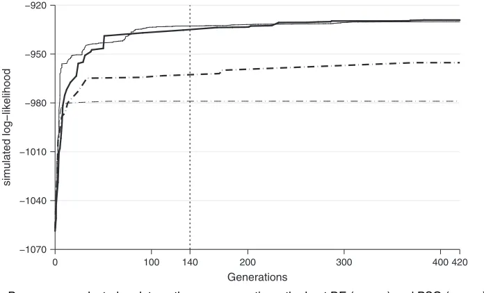
Following common practice, we setP=10KwhereKis the number of estimated parameters. We also setG=10K, as preliminary experimentation with simulated data sets suggested that both algorithms tended to slow down substantially around the 10Kth generation. To illustrate this slowdown in an empirical context, Fig. 1 plots how a selection of DE and PSO starting points that were used in the first case-study (Pap smear) would have varied ifGhad been set to 420 (or 30K) instead of 140 (or 10K). It should be emphasized that the DE and PSO solutions at the 10Kth generation are used as starting points for further optimization, not as the final solutions. All the final solutions are obtained by executing the gradient-based algorithm from the DE and PSO starting points.
The initial population ofPsolutions is generated as follows. For the generalized multinomial logit parameters to be estimatedω={β,τ,γ,σ}, consider the bounds given byl={bMNL, 0, 0,0} andu={3bMNL, 2, 1, 1:5bMNL}, wherebMNLis the vector of the MNL estimates and0is theK -vector of 0s. For each initial solution, each element ofωis independently drawn from a uniform variable lying between the corresponding elements oflandu.
The updating process of each algorithm requires two tuning parameters as additional user inputs: amplification factorF and cross-over probability Cr in the case of DE, or the acceler-ation constantCand the inertia weightDin the case of PSO. We follow Gilli and Schumann (2010) in experimenting with 16 pairs, or configurations, of those tuning parameters per al-gorithm: a DE configuration is inF={0:2, 0:4, 0:6, 0:8}×Cr={0:2, 0:4, 0:6, 0:8}, whereas a PSO configuration is inC={0:5, 1:0, 1:5, 2:0}×D={0:5, 0:75, 0:9, 1:0}. The resulting configu-rations are spaced sufficiently broadly to provide indicative evidence for future applications on what tuning parameter values could be narrowly searched over for further fine-tuning of each algorithm.
initializa-−1070 −1040 −1010 −980 −950 −920
s
im
u
l
a
ted log−likelihood
0 100 140 200 300 400 420
[image:9.485.78.426.58.269.2]Generations
Fig. 1. Pap smear—selected update paths over generations: the best DE ( ) and PSO ( ) and worst DE ( ) and PSO ( ) refer to the DE and PSO starting points that led to the best and worst final solutions in the Pap smear case-study in Section 4.3; the figure plots how these starting points had been updated until the 140th generation, at the end of which they were passed to the gradient-based algorithm for further optimization to obtain the final estimation results; the figure also plots what these starting points would have become if the algorithm continued without termination until the 420th generation
Table 2. Pap smear: conventional solutions†
Starting point logL g∞ gH−1g κ(H)
MIXL −931:065 8:64×10−7 −2:06×10−14 998.8549 GMNL-II −931:065 2:92×10−5 −4:29×10−11 998.9412 SMNL −932:133 5:46×10−8 −5:30×10−16 606.9426 GMNL-I −934:091 1:95×10−7 −2:12×10−14 4732.774 MNL −960:317 13.04914 −9:22×10−6 1:72×1018‡
†logL,gandH refer to the simulated log-likelihood, its gradient (as a column vector) and Hessian respectively. The infinity norm ofg,g∞, is the largest element ofgin absolute value.κ.H/is the 2-norm condition number ofH, defined asλmax/λminwhereλmaxandλminare the largest and smallest eigenvalues of−H. ‡His ill conditioned (i.e.κ.H/ >6:7×10⁷).
tion. We have obtained 48 DE starting points and 48 PSO starting points, by restarting each configuration three times from the same set of three seeds. In other words, the same set of three different initial populations has been used to obtain the three starting points that are associated with each configuration of each algorithm.
4.3. Results: Pap smear
[image:9.485.103.389.347.438.2]Table 3. Pap smear: 10 best DE-assisted solutions†
F Cr logL g∞ gH−1g κ(H)
0.8 0.6 −925.378 1:44×10−7 −1:78×10−15 2033.113 0.8 0.2 −925.378 9:77×10−7 −1:22×10−14 2033.185 0.8 0.2 −925.378 6:64×10−5 −3:18×10−11 2033.347 0.6 0.6 −925.378 8:07×10−5 −1:35×10−10 2033.3
0.6 0.4 −925.378 0.0001 −2:21×10−10 2033.109
0.8 0.2 −925.378 0.000438 −3:75×10−9 2033.296
0.8 0.4 −925.409 3:92×10−7 −3:02×10−15 3018.498 0.8 0.4 −925.409 9:32×10−5 −2:26×10−10 3018.577
0.6 0.2 −926.308 5:84×10−6 −1:37×10−11 936.3411
0.6 0.2 −926.308 0.00062 −4:03×10−8 936.369
[image:10.485.113.369.264.404.2]†F, Cr,C andDindicate tuning parameter values leading to relevant starting points. logL is in italics if it is greater than the highest logL (MIXL starting point) in Table 2. See the footnote to Table 2 for other information.
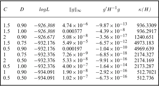
Table 4. Pap smear: 10 best PSO-assisted solutions†
C D logL g∞ gH−1g κ(H)
1.5 0.90 −926.308 4:74×10−6 −9:87×10−13 936.3309
1.5 1.00 −926.308 0.000377 −4:39×10−8 936.2917
2 0.90 −926.671 5:08×10−8 −3:56×10−17 1240.651
1.5 0.75 −932:176 5:49×10−5 −6:57×10−12 4973.183 0.5 0.90 −932:176 0.000197 −1:04×10−10 4969.639 1 0.75 −932:376 7:26×10−9 −6:85×10−18 2174.327 2 0.50 −932:376 5:33×10−8 −9:91×10−16 2174.169 0.5 1.00 −932:376 4:00×10−7 −1:64×10−14 2173.287 1 0.90 −934:091 1:90×10−8 −2:92×10−16 512.7021 0.5 0.50 −934:091 1:02×10−7 −6:73×10−16 512.736
†F, Cr,C andDindicate tuning parameter values leading to relevant starting points. logL is in italics if it is greater than the highest logL (MIXL starting point) in Table 2. See the footnote to Table 2 for other information.
Table 2 reports in descending order the simulated log-likelihood values logL of the solutions that were obtained by applying the conventional strategy, along with the usual diagnostics for checking convergence to a local optimum. Stata classifies all solutions as ‘converged’, implying that the Hessian H is negative definite and the weighted gradient norm gH−1g is smaller than−1×10⁻⁵in magnitude. Further inspection suggests that only the MNL-based solution gives warning signs: the inf-norm of the gradient,g∞, deviates far from 0 and the Hessian condition number,κ.H/, exceeds 1 over the square root of Stata’s machine precision. But this is the worst solution which is unlikely to be reported by a practitioner who tries alternative starting points.
The DE- and PSO-assisted estimation strategies find several solutions which improve on the best conventional solution. The best solution is a DE-assisted solution resulting in logL = −925:378. Table OA1 in the on-line appendix reports the logL-results from all three starts of 16 configurations of each algorithm. The main features of those results may be summarized as follows. 16 of 48 DE-assisted solutions (35%) result in logL>−931:065, ranging from−928:034 to−925:378. Considering that some of the 48 solutions include those resulting from configu-rations that are not well suited to the present application, a prima faciecase exists that the DE-assisted strategy is a practically useful complement to the conventional strategy. In con-trast, only three out of 48 PSO-assisted estimation runs (6%) result in an improved solution, ranging from−926:671 to−926:308.
Another practically attractive feature of the DE-assisted solutions is clearer indicative evi-dence on which configurations are likely to work well. Tables 3 and 4 report the top 10 logL-values found with the aid of each algorithm for DE and PSO respectively. A qualitative direction for fine-tuning the DE configuration to the present application would be ‘try a big change to the parameter estimates, but accept the resulting change only occasionally’. No similar direction emerges in the case of PSO, as the top 10 solutions are associated with a wider range of configu-rations. To be specific, the top 10 DE-assisted solutions are overly represented by configurations specifying a large amplification factorF (0.6 and 0.8) and a small cross-over probability Cr (0.2 and 0.4). When restricting attention to the four implied configurations, nine out of 12 DE-assisted estimation runs (75%) find an improved solution, and four of those nine runs reach the highest logL of−925:378. In contrast, a smallF(0.2 and 0.4) appears not well suited, regardless of the accompanying Cr: only two of such 28 DE-assisted runs find an improved solution, none of them reaching the highest logL.
The highest logL has been reached from six different DE starting points and displays ap-propriate convergence diagnostics. Of course, as in the case of the best conventional solution, such repeatability does not imply that the underlying solution is the global maximum. Verifying that a particular solution is the global maximum is considered to be beyond the scope of our study because, as far as we are aware, no definitive guideline exists on how such verification is to be performed. We have, however, verified that the best conventional solution is not the global maximum. Our present and subsequent analysis focuses on the consequences of basing an empirical analysis on the best conventional solution when a DE- or PSO-assisted solution is capable of achieving a higher logL.
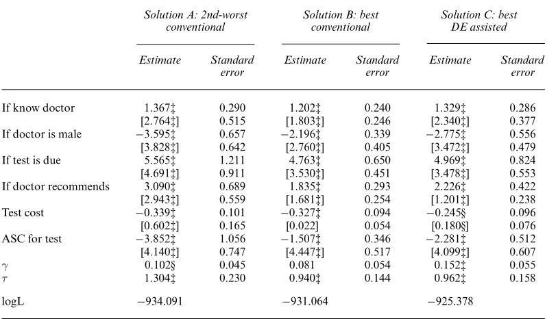
Table 5 reports parameter estimates at the second-worst and best conventional solutions, and at the best DE-assisted solution. The second-worst conventional solution (solution A) results from the GMNL-I starting point, and is the worst out of the conventional solutions with acceptable convergence diagnostics. In terms of logL, the best conventional solution (solution B) gains over solution A by about 3 points, and there are marked differences between the coefficient estimates: the mean of the ‘alternative-specific constant test’, in particular, is about 2.5 times larger in solution A than in solution B (−3:85versus−1:51) and many other estimates disagree even on the first significance figures.
Table 5. Pap smear: generalized multinomial logit parameter estimates†
Solution A: 2nd-worst Solution B: best Solution C: best
conventional conventional DE assisted
Estimate Standard Estimate Standard Estimate Standard
error error error
If know doctor 1:367‡ 0.290 1:202‡ 0.240 1:329‡ 0.286 [2:764‡] 0.515 [1:803‡] 0.246 [2:340‡] 0.377 If doctor is male −3:595‡ 0.657 −2:196‡ 0.339 −2:775‡ 0.556 [3:828‡] 0.642 [2:760‡] 0.405 [3:472‡] 0.479 If test is due 5:565‡ 1.211 4:763‡ 0.650 4:969‡ 0.824 [4:691‡] 0.911 [3:530‡] 0.451 [3:478‡] 0.553 If doctor recommends 3:090‡ 0.689 1:835‡ 0.293 2:226‡ 0.422 [2:943‡] 0.559 [1:681‡] 0.254 [1:201‡] 0.238 Test cost −0:339‡ 0.101 −0:327‡ 0.094 −0:245§ 0.096 [0:602‡] 0.165 [0.022] 0.054 [0:180§] 0.076 ASC for test −3:852‡ 1.056 −1:507‡ 0.346 −2:281‡ 0.512 [4:140‡] 0.747 [4:447‡] 0.517 [4:099‡] 0.607
γ 0.102§ 0.045 0.081 0.054 0:152‡ 0.055
τ 1:304‡ 0.230 0:940‡ 0.144 0:962‡ 0.158
logL −934:091 −931:064 −925:378
†For each named attribute, the corresponding elements ofβandσ(in square brackets) are reported. The ‘2nd-worst conventional’ and ‘best conventional’ respectively refer to GMNL-I and MIXL or GMNL-II starting point solutions in Table 2. ‘Best DE assisted’ refers to the first six solutions in Table 3.
‡Statistical significance at the 1% level. §Statistical significance at the 5% level.
(WTP) and the predicted choice probability, would be substantively different. (The WTP for a specific attribute is the utility coefficient on that attribute divided by the absolute value of the utility coefficient on the price or cost attribute. The WTP distribution can be simulated first by making simulated draws for all utility coefficients according to equation (2), and then computing relevant ratios of those simulated coefficients.)
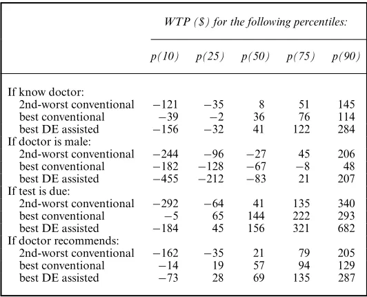
To facilitate further comparisons, Table 6 reports selected percentiles of WTP distributions simulated from solutions A, B and C. As expected from the earlier comparison of A with B, these two solutions imply quite a different median WTP, which is the primary statistic on which practitioners are likely to focus (e.g. Smallet al. (2005)). The implied WTP distributions of solution B and C, in contrast, are only slightly different at the median. The main difference between those two solutions is that, because of heterogeneity in the cost coefficient which is only picked up by solution C, the interpercentile ranges of WTP are much more pronounced for C than B. As a result, conclusions regarding the dispersion of the WTP distribution that is implied by solution B may require reconsideration.
Table 6. Pap smear: simulated WTP distributions†
WTP ($) for the following percentiles:
p(10) p(25) p(50) p(75) p(90)
If know doctor:
2nd-worst conventional −121 −35 8 51 145 best conventional −39 −2 36 76 114 best DE assisted −156 −32 41 122 284 If doctor is male:
2nd-worst conventional −244 −96 −27 45 206 best conventional −182 −128 −67 −8 48 best DE assisted −455 −212 −83 21 207 If test is due:
2nd-worst conventional −292 −64 41 135 340 best conventional −5 65 144 222 293 best DE assisted −184 45 156 321 682 If doctor recommends:
2nd-worst conventional −162 −35 21 79 205 best conventional −14 19 57 94 129 best DE assisted −73 28 69 135 287
†Each WTP distribution has been simulated by making 100000 draws from the joint density of utility coefficients according to the solutions in Table 5.
p.Q/denotes theQth percentile of the simulated distribution.
Table 7. Pap smear: predicted choice probabilities†
Solution A Solution B Solution C
Base choice probability 0.45 0.57 0.53 Change when test is not due −0:24 −0:27 −0:26 Change when does not know −0:06 −0:06 −0:07
doctor
Change when doctor is female 0.15 0.12 0.15 Change when doctor 0.12 0.09 0.11
recommends
Change when test cost is 0 0.04 0.05 0.04
†Solutions A, B and C are respectively based on 100000 draws from the joint density of utility coefficients according to the ‘2nd-worst conventional’, ‘best conventional’ and ‘best DE-assisted’ solutions in Table 5. The base choice probability is the probability of choosing a test (over no test) when the test is due, the patient knows the doctor, the doctor is male, the doctor makes no recommendation and the cost is $30. Each row reports how this probability changes when each attribute changes from its base level.
than B (0.57) and C (0.53). This robustness may stem from the same source as the difficulties of finding the global maximum, namely that different combinations of parametric values lead to similar probabilities or likelihoods.
4.4. Results: pizza A data
[image:13.485.114.382.344.461.2]Table 8. Pizza A: conventional solutions†
Starting point logL g∞ gH−1g κ(H)
GMNL-II −1361:84 1:45×10−5 −4:88×10−12 173280.2 MIXL −1365:17 1:30×10−6 −1:58×10−12 20000.77 MNL −1368:44 3:98×10−5 −1:51×10−9 182428.5 GMNL-I −1374:45 0.003018 −1:71×10−8 3409.606 SMNL −1395:5 4:60×10−6 −8:35×10−13 442.66
[image:14.485.101.382.206.351.2]†See the footnote to Table 2.
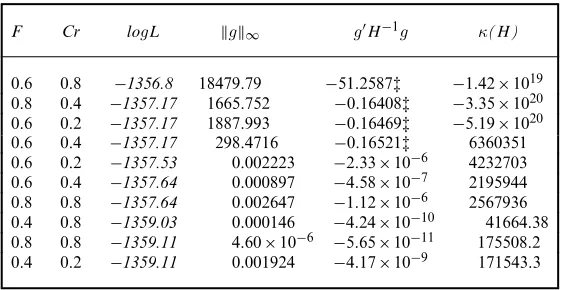
Table 9. Pizza A: 10-best DE-assisted solutions†
F Cr logL g∞ gH−1g κ(H)
0.6 0.8 −1356.8 18479.79 −51:2587‡ −1:42×1019
0.8 0.4 −1357.17 1665.752 −0:16408‡ −3:35×1020
0.6 0.2 −1357.17 1887.993 −0:16469‡ −5:19×1020
0.6 0.4 −1357.17 298.4716 −0:16521‡ 6360351
0.6 0.2 −1357.53 0.002223 −2:33×10−6 4232703
0.6 0.4 −1357.64 0.000897 −4:58×10−7 2195944
0.8 0.8 −1357.64 0.002647 −1:12×10−6 2567936
0.4 0.8 −1359.03 0.000146 −4:24×10−10 41664.38
0.8 0.8 −1359.11 4.60×10⁻⁶ −5:65×10−11 175508.2
0.4 0.2 −1359.11 0.001924 −4:17×10−9 171543.3
†logL is in italics if it is greater than the highest logL (GMNL-II starting point) in Table 8. See the footnotes to Table 2 for other information.
‡Stata declared convergence failure since|gH−1g|exceeds the tolerance criterion
(1×10⁻⁵).
the mean and standard deviation of the canonical random coefficient on each attribute results in 18 generalized multinomial logit parameters.
Table 8 reports logL-values attained by the conventional solutions. The MIXL and GMNL-II starting points again turn out to be two best conventional starting points. But, this time, only GMNL-II leads to the highest logL of−1361:84. All conventional solutions, including the worst, display acceptable convergence diagnostics.
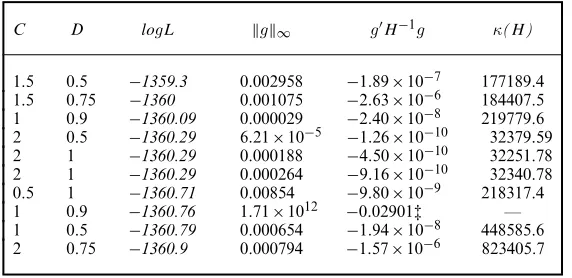
Tables 9 and 10 report the top 10 logL-values attained by respectively the DE- and PSO-assisted solutions. The full set of the DE- and PSO-PSO-assisted estimation runs are available in Table OA2 of the on-line appendix. The results agree with the Pap smear results on two broad conclusions. First, the best solution (logL= −1356:80) is obtained by the DE-assisted strategy. Second, the DE-assisted strategy outperforms the PSO-assisted strategy in terms of finding a solution improving on the best conventional solution: 42% or 20 out of 48 DE-assisted solutions, and 23% or 11 out of 48 PSO-assisted solutions, improve on the best conventional solution.
The current results, however, are quite different from the previous results in one important dimension. 11 DE-assisted solutions (23%) and four PSO-assisted solutions (8%) were declared ‘not converged’ by Stata, because the associated Hessian is not negative definite and/orgH−1g
exceeds the tolerance level. Importantly, as the upper panel of Table 9 shows, the clear sign of non-convergence is present in the four best solutions that we have obtained.
Table 10. Pizza A: 10 best PSO-assisted solutions†
C D logL g∞ gH−1g κ(H)
1.5 0.5 −1359.3 0.002958 −1:89×10−7 177189.4
1.5 0.75 −1360 0.001075 −2:63×10−6 184407.5
1 0.9 −1360.09 0.000029 −2:40×10−8 219779.6
2 0.5 −1360.29 6:21×10−5 −1:26×10−10 32379.59
2 1 −1360.29 0.000188 −4:50×10−10 32251.78
2 1 −1360.29 0.000264 −9:16×10−10 32340.78
0.5 1 −1360.71 0.00854 −9:80×10−9 218317.4
1 0.9 −1360.76 1:71×1012 −0:02901‡ —
1 0.5 −1360.79 0.000654 −1:94×10−8 448585.6
2 0.75 −1360.9 0.000794 −1:57×10−6 823405.7
†logL is in italics if it is greater than the highest logL (GMNL-II starting point) in Table 8. See the footnotes to Table 2 for other information.
‡Stata declared convergence failure since|gH−1g|exceeds the tolerance criterion (1×10⁻⁵).
of Chiou and Walker (2007) and re-estimated the model with a higher number of simulation draws (10 000), using as starting point the best conventional solution. As Chiou and Walker pointed out, using a larger number of draws unmasks empirical underidentification: whereas the best conventional solution displays acceptable convergence diagnostics at 500 draws, the new estimation run failed to attain convergence. Thus, in the present application, the use of the DE-and PSO-assisted strategies leads to a practically different implication from the conventional strategy: namely that the model needs to be simplified before the parameter estimates can be readily interpreted.
5. Further analysis
The results that were described in the previous section suggest that the DE- and PSO-assisted estimation strategies can be a useful tool for improving the chance of finding the global maximum in empirical applications. Between the two strategies, the DE-assisted strategy appears to be the better choice since it improves on the conventional solution more frequently and is more consistent in terms of which configurations are likely to perform well. The best conventional and DE-assisted solutions have led to somewhat (Pap smear) and quite (pizza A) different substantive conclusions based on the estimated generalized multinomial logit models.
The on-line appendix reports an extensive set of results from further case-studies, which echo the relatively superior performance of the DE-assisted strategy. The additional case-studies include applications of the DE- and PSO-assisted strategies to two larger empirical data sets (holiday A and mobile phone) of Fiebiget al. (2010), as well as to simulated data sets. We also reanalyse the Pap smear and pizza A data sets, using alternative hybrid estimation strategies which exploit the DE and PSO algorithms jointly with the Nelder–Mead algorithm. (We thank a reviewer for this suggestion.) Finally, we repeat all of our four empirical case-studies in the new context of estimation of the mixed logit model, MIXL, instead of the generalized multinomial logit model.
6. Conclusion
obtain starting values for random parameter logit models. Our findings suggest that the DE-assisted strategy can be a very effective tool to diagnose the adequacy of the modelling results that are obtained by using the conventional strategy. The DE configuration (F=0:8, Cr=0:2) performs particularly well and may serve as a baseline configuration in similar applications.
Our results clearly suggest that repeatedly finding a particular maximum from several starting points is not reliable evidence that it is the global maximum. Given the difficulties of verifying the global maximum in empirical work, it is prudent to embrace the recommendation that Knittel and Metaxoglou (2014) made in a different context of non-linear optimization: namely to report the main differences across several optima found during the estimation process.
We conclude with a few remarks on the estimation run time of the DE-assisted strategy relative to that of the conventional strategy. Comparing the run time is inherently difficult because the estimation issue of interest is not to locate a unique maximum in the fastest time but to locate the best of several possible maxima. The sensitivity of a gradient-based optimizer’s run time to starting points poses another source of complication: in the Pap smear case-study, for example, conventionally estimating the generalized multinomial logit model took as little as 17 min (from the MIXL starting point) to 11 h (from the MNL starting point). With thesecaveatsin mind, we note that, in all of our empirical case-studies, two DE-assisted estimation runs using (F=0:8, Cr=0:2) required a comparable amount of time with that of the conventional strategy of searching over major special cases of the final model: continuing with the Pap smear example, each DE-assisted run using this configuration took 1.5 h whereas the conventional strategy took a combined total of 3.5 h even when we overlook the exceptional 11-h run from the MNL starting point. In every empirical case-study and given the same configuration, at least two out of three restarts of the DE-assisted strategy located a higher maximum than the conventional strategy. These findings suggest that running two or three restarts of the DE-assisted strategy would make an effective and computationally feasible addition to the empirical practitioner’s toolkit.
Acknowledgements
We thank the Joint Editor, the Associate Editor and two reviewers for their very helpful com-ments and suggestions. We also thank Jin Yan for alerting us to the literature on population-based optimization heuristics, seminar participants at Copenhagen Business School and the Universities of Aberdeen, Durham and Leeds, and attendees at the Fourth International Choice Modelling Conference.
References
Chiou, L. and Walker, J. (2007) Masking identification of discrete choice models under simulation methods.J. Econmetr.,141, 683–703.
Das, S. and Suganthan, P. (2011) Differential evolution: a survey of the state-of-the-art.IEEE Trans. Evoln. Computn,15, 4–31.
Dorsey, R. and Mayer, W. (1995) Genetic Algorithms for estimation problems with multiple optima, nondiffer-entiability, and other irregular features.J. Bus. Econ. Statist.,13, 53–66.
Eberhart, R. and Kennedy, J. (1995) A new optimizer using particle swarm theory. InProc. 6th Int. Symp. Micromachine and Human Science, pp. 39–43.
Fiebig, D., Keane, M., Louviere, J. and Wasi, N. (2010) The generalized multinomial logit model: accounting for scale and coefficient heterogeneity.Marktng Sci.,29, 393–421.
Gilli, M. and Schumann, E. (2010) Robust regression with optimisation heuristics. InNatural Computing in Computational Finance, vol. 3 (eds A. Brabazon and M. O’Neill), pp. 9–30. Berlin: Springer.
Greene, W. and Hensher, D. (2010) Does scale heterogeneity across individuals matter?: an empirical assessment of alternative logit models.Transportation,37, 413–428.
Gu, Y., Hole, A. and Knox, S. (2013) Fitting the generalized multinomial logit model in Stata.Stata J.,13, 382–397.
Harding, M. and Hausman, J. (2007) Using a Laplace approximation to estimate the random coefficients logit model by nonlinear least squares.Int. Econ. Rev.,48, 1311–1328.
Huber, J. and Train, K. (2001) On the similarity of Classical and Bayesian estimates of individual mean partworths. Marktng Lett.,12, 259–269.
Johar, M., Fiebig, D., Haas, M. and Viney, R. (2013) Using repeated choice experiments to evaluate the impact of policy changes on cervical screening.Appl. Econ.,45, 1845–1855.
Keane, M. and Wasi, N. (2013) Comparing alternative models of heterogeneity in consumer choice behavior.J. Appl. Econmetr.,28, 1018–1045.
Knittel, C. and Metaxoglou, K. (2014) Estimation of random-coefficient demand models: two empiricists’ per-spective.Rev. Econ. Statist.,96, 34–59.
Knox, S., Viney, R., Gu, Y., Hole, A., Fiebig, D., Street, D., Haas, M., Weisberg, E. and Bateson, D. (2013) The effect of adverse information and positive promotion on women’s preferences for prescribed contraceptive products.Socl Sci. Med.,83, 70–80.
McFadden, D. and Train, K. (2000) Mixed MNL models for discrete response.J. Appl. Econmetr.,15, 447–470. Revelt, D. and Train, K. (1998) Mixed logit with repeated choices: households’ choices of appliance efficiency
level.Rev. Econ. Statist.,80, 647–657.
Small, K., Winston, C. and Yan, J. (2005) Uncovering the distribution of motorists’ preferences for travel time and reliability.Econometrica,73, 1367–1382.
StataCorp. (2011)Stata Statistical Software: Release 12. College Station: StataCorp.
Storn, R. and Price, K. (1997) Differential evolution—a simple and efficient heuristic for global optimization over continuous spaces.J. Globl Optimizn,11, 341–359.
Train, K. (2008) EM algorithms for nonparametric estimation of mixing distributions.J. Choice Modllng,1, 40–69. Train, K. (2009)Discrete Choice Methods with Simulation, 2nd edn. New York: Cambridge University Press.
Supporting information
Additional ‘supporting information’ may be found in the on-line version of this article: