Probabilistic Analysis of Different Methods Used to Compute the Failure Pressure of Corroded Steel Pipelines

Int. J. Electrochem. Sci., 8 (2013) 11356 - 11370

International Journal of

ELECTROCHEMICAL

SCIENCE

Technical report

Probabilistic Analysis of Different Methods Used to Compute

the Failure Pressure of Corroded Steel Pipelines

J.C. Velazquez1*, F. Caleyo2, J.M. Hallen2, O. Romero-Mercado3, H. Herrera-Hernández4,

1

Instituto Politécnico Nacional, Departamento de Ingeniería Química Industrial, ESIQIE, U.P. Adolfo López Mateos, Zacatenco, 07738 México, D.F., México

2

Instituto Politécnico Nacional, Departamento de Ingeniería Metalúrgica, ESIQIE, U.P. Adolfo López Mateos, Zacatenco, 07738 México, D.F., México

3

Pemex- Refinación, Coordinación de Proyectos de Impacto Social y Alta Rentabilidad (CPISAR), 4to piso, Torre Titano, Anáhuac, 11311, México D.F., México

4 _{Universidad Autónoma del Estado de México, C.U. Valle de México, Ingeniería Industrial. Blvd.}

Universitario s/n, Predio San Javier Atizapán de Zaragoza 54500, México

*

E-mail: jcva8008@yahoo.com.mx

Received: 16 May 2013 / Accepted: 2 July 2013 / Published: 20 August 2013

For many years, different methods for computing the failure pressure of buried pipelines that transport crude oil, natural gas or any hydrocarbon derivative have been regularly implemented; however, these methods work with variables affected by uncertainty. Therefore, in this paper, the authors present a Monte Carlo methodology to evaluate the probabilistic behavior of several failure pressure methods in order to estimate their effect in the probability of failure calculations from the information published by the Pipeline Research Council International (PRCI) for the actual failure pressure of corroded pipelines.

Keywords: Carbon steel, failure pressure, corroded steel pipeline, probabilistic analysis, Monte Carlo Simulation

1. INTRODUCTION

several methods for computing the pipeline failure pressure have been developed in order to determine more accurately what kind of defects cause a greater risk of failure [4-10]. However, all the well-known methods used in the oil and gas industry to calculate the failure pressure are merely deterministic models. It means that they do not take into account the randomness of the input variables involved. Some of these random variables are consequence of the steel pipe manufacturing process, such as diameter, wall thickness, yield strength and ultimate tensile strength. The uncertainty in other variables like defect length and defect depth are resulted from measurement errors [11]. Taking into account the uncertainty of the input variables, it is possible to create failure pressure histograms for each method. Having a failure pressure histogram and the working pressure histogram, it is feasible to compute the probability of failure. Nowadays, the value of probability of failure has a great importance in the pipeline maintenance programs, due to the fact that pipeline operators tend to use a probability of failure threshold to manage the risk and the cost of maintenance.

The information published by the Pipelines Research Council International [12] regarding the results of burst tests of corroded pipeline sections is used in this work. The randomness characteristic of each input variable is taken into consideration to build the failure pressure histogram for each failure pressure method. All the failure pressure histograms are fitted to some theoretical probability distributions. As all the data used in this research come from pipes that failed at burst test, it is possible to determine the probability of failure of pipes that have already failed. This research aims to discuss any possible threshold of probability of failure that can be useful for people that manage the pipeline risk.

2. EXPERIMENTAL PROCEDURE

2.1 Calculating The Pipeline Failure Pressure.

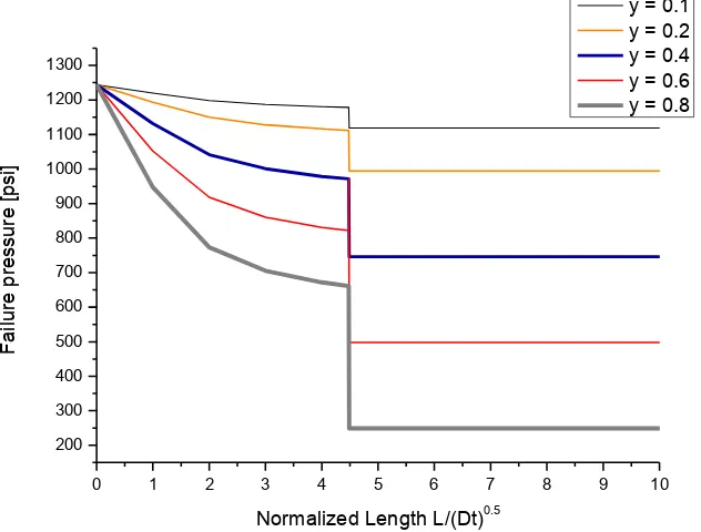
The most well-known methods to compute remaining strength in hydrocarbon transmission pipelines are the ASME B31G [4] and RSTRENG [5] models. These failure equations are based on fracture mechanic principles. Nevertheless, there are other methods like PCORRC [6,7], LPC-1 [8], Shell 92 [9], and Fitnet FSS [10] that also calculate the failure pressure of corroding pipeline sections. In Mexico, Pemex (National Oil Company) has established some guidelines about when each method should be used [13]. The methods aforementioned and the corresponding nomenclatures are listed in Table I and Table II, respectively.

Table I. Failure pressure methods for pressurized pipes with active corrosion defects.

Failure pressure methods Mathematical expressions

B31G M 1 0.893L

Dt

 

2y 1

2YSt _3t L

pf 1.11 for 4.479

2y 1

D ₁ Dt

3t M

2YSt y L

pf 1.11 1 for 4.479

D t Dt

 _         _         _  _    RSTRENG-1 y 1 0.85

2(YS 68.95MPa)t _t

pf y 1 D 1 0.85 t M  _         _      2 4 2 2 2 L L

M 1 0.6275 0.003375 for L / Dt 50

Dt D t

   

2

2

L

M 0.032 3.3 for L / Dt 50

Dt

  

PCORRC (Batelle)

2UTSt y

pf 1 M

D t

 

 _  _

 

L

M 1 exp 0.157

D(t d) / 2

 

  _ _



 

LPC-1 (DNV-99) _2UTSt 1 y

t pf y 1 D t 1 t M  _        _{ } _   2 L M 1 0.31

Dt   Shell-92 y 1 1.8UTSt _t pf y 1 D 1 t M  _        _      2 L M 1 0.805

Dt

 

Fitnet FSS 65/ YS

y 1

2UTSt(1 / 2) _t

pf

y 1

D t ₁

t M  _        _{  }     2 L M 1 0.8

Dt

 

Table II. Nomenclature.

Symbol Definition Symbol Definition

D Outside (external) diameter PF Probability of failure

y Defect depth LSF Limit State Function

t Pipe wall thickness N Number of Monte Carlo

simulation

L Defect length

np

 Nonparametric mean

YS Yield strength _np Nonparametric standard

deviation

UTS Ultimate tensile strength - -

pf Failure pressure - -

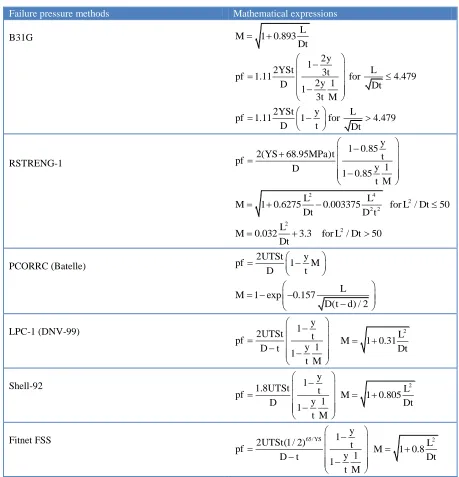
Given this characteristic (positive skew), each histogram was fitted to GEVD (Generalized Extreme Value Distribution). It is important to remember that the GEVD probability density function (pfd) can represent histograms that show positive and negative skew.

The positive skew characteristic and the numerical value of the mode in the “error histogram” confirm the fact that the most probable value of the error is greater than 1. It means that the real failure pressure is greater than the predicted failure pressure in most of the cases. Figure 1 illustrates the error distribution obtained by the Fitnet FSS method, while Table III shows the results of the “error histogram” fitted to the GEVD for each pipeline failure pressure method.

Figure 1. Error histogram for the Fitnet FSS method and the corresponding GEVD.

Table III. Error Histogram fitted to GEVD for each method.

1/ k

x loc

F(x) exp 1 k

scl



 _{  } 

 _ _{ } _

 

 

Method Location parameter

(loc)

Shape parameter (k)

Scale parameter (scl)

B31G 1.163 0.324 0.278

RSTRENG-1 1.098 0.194 0.232

PCORRC 0.994 0.309 0.302

LPC-1 0.969 0.238 0.231

SHELL-92 1.250 0.230 0.288

FITNET FSS 1.188 0.250 0.265

1.0 1.5 2.0 2.5 3.0 3.5

0.000 0.036 0.073 0.109 0.146 0.182 0.219

0.255 _{Error distribution Fitnet FSS method.}

Histogram GEVD

D

e

n

si

ty

o

f

Prob

a

b

ili

ty

2.2. Uncertainty of the variables.

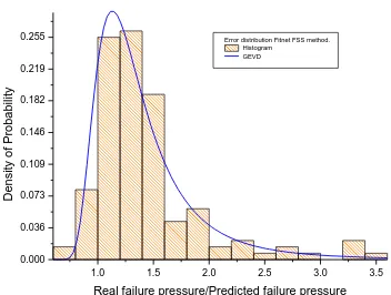
The real physical properties and characteristics of a pipe are unknown. The material properties vary along the pipe length. These variations depend on the material quality and the manufacturing process. Therefore, it is practically impossible to assess the pipeline integrity from the actual pipeline characteristics. For this reason, the pipeline material specifications use a minimum value for the steel characteristics, such as minimum yield strength or minimum ultimate tensile strength. For example, in the API 5L specifications, the X52 grade refers to a pipeline steel that must have at least 52000 psi yield strength as minimum [14]. Nonetheless, the question arises whether it is possible to estimate the failure pressure taking into account the uncertainty level of the yield strength, UTS, diameter, pipe wall thickness, and defect depth and length. However, the only way to take into account these uncertainties is applying computational methods like Monte Carlo simulations. To use the Monte Carlo simulations, it is necessary to do a probabilistic analysis to account for the randomness of the input variables. Table IV presents the input variables used to compute the failure pressure (in this case random variables) and their associated probability distributions.

By using the theoretical distributions of the input variables, it is possible to generate the failure pressure histograms through the Monte Carlo method. This numerical method is useful to create random numbers and evaluate deterministic mathematical expressions such as all the failure pressure methods. In 2002, F. Caleyo and coworkers [15] concluded that the variable that exerts the greatest influence on the failure pressure is the defect depth. For this reason, one of the purposes of this research is to determine if there is any relationship between the shape of the failure pressure distribution and the defect depth distribution.

Table IV. Distribution of the variables used in the failure pressure methods.

Variable Distribution Coefficient of

Variation

Reference

D Normal 0.06% [19]

YS LogNormal 3.5% [19]

UTS LogNormal 3.5% [19]

t Normal 1% [19]

y Normal 15% [20]

L Normal 10% [20]

Operating pressure Gumbel 5% Established by

PEMEX

3. RESULTS AND DISCUSSION

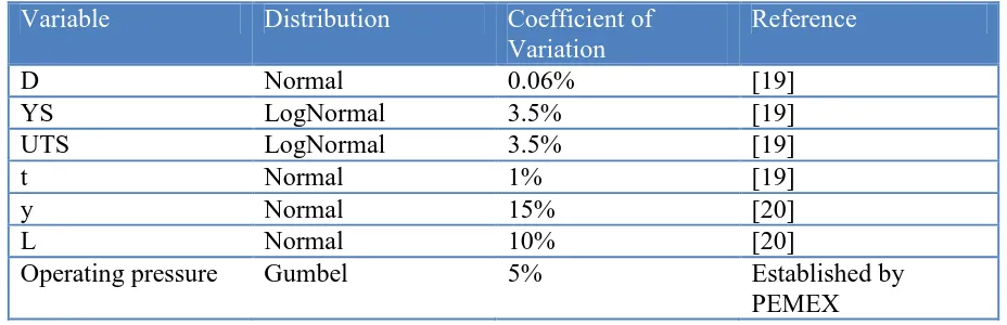
4.479. The magnitude of this discontinuity increases as the defect depth increases, as the Figure 3 shows.

Figure 2. Failure pressure distribution for the case where y/t=0.706, L / Dt4.827, D/t = 64.1 and YS= 36000 psi.

0 1 2 3 4 5 6 7 8 9 10

200 300 400 500 600 700 800 900 1000 1100 1200 1300

F

a

ilu

re

p

re

ssu

re

[p

si

]

Normalized Length L/(Dt)0.5

y = 0.1 y = 0.2 y = 0.4 y = 0.6 y = 0.8

Figure 3. Failure pressure against normalized defect length for: D/t = 64.1 and YS= 36000 psi.

From the report published by PRCI [12], only 138 cases were considered in this study, because these cases show all the information needed to assess the defects by means of all the above mentioned methods. For each one of these 138 cases, and for each failure method, it was generated a failure pressure histogram.

0 500 1000 1500 2000 2500 3000

0.0000 0.0025 0.0050 0.0075 0.0100 0.0125 0.0150 0.0175 0.0200 0.0225 0.0250 0.0275 0.0300 0.0325 0.0350

D

e

n

si

ty

o

f

Prob

a

b

ili

ty

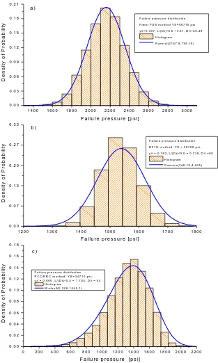
All the generated failure pressure histograms were fitted to the Weibull, Gamma and Normal distribution functions. It is important to mention that the goodness of fit test used was the Kolmogorv-Smirnov test. For the sake of illustration, Figure 4 exemplifies the fitting of the failure pressure histograms to different probability density functions.

1 4 0 0 1 6 0 0 1 8 0 0 2 0 0 0 2 2 0 0 2 4 0 0 2 6 0 0 2 8 0 0 3 0 0 0 0 .0 0

0 .0 3 0 .0 6 0 .0 9 0 .1 2 0 .1 5 0 .1 8 0 .2 1

D e n s it y o f P ro b a b il it y

F a ilu r e p r e s s u r e [p s i]

F a ilu re p re s s u re d is tr ib u tio n F itn e t F S S m e th o d Y S = 6 6 7 1 6 p s i y /t= 0 .3 9 7 , L /(D t)^ 0 .5 = 3 .5 1 , D /t= 4 9 .4 8

H is to g ra m N o r m a l(2 1 5 7 .8 ,1 9 6 .1 6 )

a )

1 2 0 0 1 3 0 0 1 4 0 0 1 5 0 0 1 6 0 0 1 7 0 0 1 8 0 0 0 .0 0

0 .0 7 0 .1 3 0 .2 0 0 .2 7 0 .3 3

D e n s it y o f P ro b a b il it y

F a ilu r e p r e s s u r e [p s i]

F a ilu r e p re s s u r e d is trib u tio n B 3 1 G m e th o d Y S = 5 8 7 0 8 p s i, y /t = 0 .3 8 2 , L /(D t) ^0 .5 = 0 .7 3 8 , D /t = 8 0

H is to g ra m G a m m a (3 4 6 .1 6 ,4 .4 0 5 )

b )

0 2 0 0 4 0 0 6 0 0 8 0 0 1 0 0 0 1 2 0 0 1 4 0 0 1 6 0 0 1 8 0 0 2 0 0 0 2 2 0 0 0 .0 0

0 .0 2 0 .0 4 0 .0 6 0 .0 8 0 .1 0 0 .1 2 0 .1 4 0 .1 6 0 .1 8

D e n s it y o f P ro b a b il it y

F a ilu r e p r e s s u r e [p s i]

F a ilu r e p r e s s u re d is trib u tio n P C O R R C m e th o d . Y S = 3 4 7 1 0 p s i, y /t = 0 .6 6 6 , L /(D t)^ 0 .5 = 1 .7 4 5 , D /t = 6 4

H is to g r a m W e ib u ll(5 .3 2 8 ,1 4 4 5 .1 )

c )

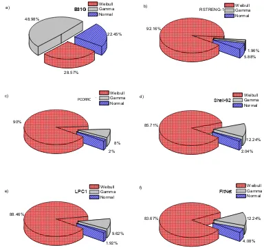
Figure 5. Pie graphs that show the rate of cases that the failure pressure histograms fit better to the theoretical distributions for defect depths equal or greater than 70% of the pipe wall thickness according to the different methods: a) B31G, b) RSTRENG-1, c) PCORRC, d) Shell-92, e) LPC1, and f) FitNET.

To analyze the influence of the corrosion defect depth on the failure pressure histograms, the cases with defects equal to or deeper than 70% of the pipe wall thickness were used. The histograms of these cases were fitted to Weibull, Normal and Gamma distributions. For the B31G method, only 28.5% of the cases with the deepest defect have the Weibull distribution as the best fitting. In contrast, in the rest of the methods the best fitting was the Weibull distribution in more than 85% of the cases. Figure 5 shows a graphic to summarize these results.

It is important to mention that the Weibull distribution can fit correctly to histograms that show negative skewness, such as the pressure failure histograms obtained for the deepest defects.

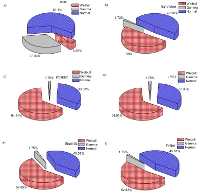
The cases where the defects are equal to or deeper than 40% but lower than 70% of the wall thickness were also studied. The failure pressure histograms were fitted to Weibull, Normal, and

22.45% 48.98%

28.57%

Weibull Gamma Normal

B31G

a)

5.88% 1.96% 92.16%

Weibull Gamma Normal RSTRENG-1

b)

2% 8% 90%

Weibull Gamma Normal

PCoor

c)

2.04% 12.24% 85.71%

Weibull Gamma Normal

Shell-92

d)

1.92% 9.62% 88.46%

Weibull Gamma Normal

LPC1

e)

4.08% 12.24% 83.67%

Weibull Gamma Normal

FitNet

f)

Gamma probability density functions. Figure 6 illustrates that the better fit were obtained for the Weibull and Normal distributions.

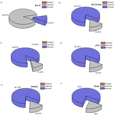
When assessing the pipes with shallow defects (<40% wall thickness) with the B31G method, it was observed that in about 80% of the cases, the best fit was for the Gamma distribution. For the rest of the methods, the Normal distribution prevails as the best fitting model. This result is illustrated in Figure 7.

Figure 6. Pie graphs that show the rate of cases that the failure pressure histograms fit better to the theoretical distributions for defect depths between 45% and 70% of the pipe wall thickness according to the different methods: a) B31G, b) RSTRENG-1, c) PCORRC, d) Shell-92, e) LPC1 and f) FitNET FSS.

From Figures 5, 6 and 7 one can notice that the corrosion defect depth has a great influence in the asymmetry of the failure pressure probability distribution function; being the deeper corrosion defects those that provoke a negative skew in the failure pressure histogram. This negative skew means that the deeper the defects are, the greater are the left tail of the failure pressure probability distribution

61.4%

33.33%

5.26% Weibull Gamma Normal a)

48.28% 1.72%

50%

Weibull Gamma Normal

B31GMod

b)

33.33% 1.75%

64.91%

Weibull Gamma Normal

PCoor

c)

33.33% 1.75%

64.91%

Weibull Gamma Normal

LPC1

d)

40.35% 1.75%

57.89%

Weibull Gamma Normal

Shell 92

e)

45.61% 1.75%

52.63%

Weibull Gamma Normal

FitNet

f)

function and the area of the PDF towards lower failure pressure values. Therefore, there are more chances that the operating pressure histogram overlaps the failure pressure histogram.

Figure 7. Pie graphs that show the rate of cases that the failure pressure histograms fit better to the theoretical distributions for defect depths smaller than 45% of the pipe wall thickness according to the different methods: a) B31G, b) RSTRENG-1, c) PCORRC, d) Shell-92, e) LPC1 and f) FitNET FSS.

3.1 Probability of Failure.

All the methods described in this paper are deterministic in nature. Therefore in order to compute the probability of failure, it is necessary to use again Monte Carlo simulations, taking into account the uncertainty in the operating pressure and the uncertainties associated with the failure pressure.

Based on reliability engineering, the limit state function (LSF) can be defined as the difference between the failure pressure (pf) and the operating pressure (pop) [16].

LSF = pf – pop (1) 13.33%

86.67%

Weibull Gamma Normal

B31G

a)

83.33%

16.67%

Weibull Gamma Normal

B31G Mod

b)

86.67%

13.33%

Weibull Gamma Normal

PCoor

c)

83.33%

16.67%

Weibull Gamma Normal

LPC1

d)

83.33%

16.67%

Weibull Gamma Normal

Shell92

e)

80%

20%

Weibull Gamma Normal

Fitnet

f)

It is possible to affirm that a pipe can work safely if LSF > 0 (pf > pop), while a failure would happen if LSF ≤ 0 (pf ≤ pop). Therefore, the probability of failure can be equated to the probability that the failure pressure is equal or lower than the operating pressure. Applying the Monte Carlo simulation framework to expression (1), it is possible to compute the probability of failure. To make this, pf and pop are treated as random variables and the expression (1) is tested N times. The number of cases was the operating (working) pressure is equal to or greater than the failure pressure gives a non-biased estimate of the probability of failure [16]:

PF = n(pf – pop ≤ 0)/ N (2)

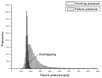
As it was mentioned before, the data used in this research corresponds to pipeline sections that failed. In the 138 selected cases, the operational pressure was considered equal to the test pressure (real failure pressure) that provokes the failure. To illustrate this, Figure 8 shows both the failure pressure histogram and the working pressure histogram. The overlapping area between the histograms represents the probability of failure.

0 1000 2000 3000 4000 5000 6000 7000 8000 9000

0 500 1000 1500 2000 2500 3000 3500 4000

4500 Working pressure

F

re

cu

e

n

cy

Failure pressure [psi]

Failure pressure

Overlapping

Figure 8. Overlapping area between failure pressure histogram and working pressure histogram. The average working pressure is 11.27 psi. The pipe characteristics are YS = 58708 psi, UTS = 76098 psi, D/t =80, L/sqrt(Dt) = 0.738 and y/t = 0.382. The method used in this example is Fitnet FSS.

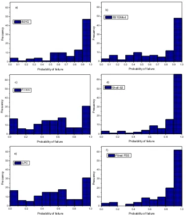
was calculated using the six failure pressure methods shown in Table 1. Figure 9 exemplifies how the probability of failure is distributed for each method.

Figure 9. Probability of failure histograms without considering the error of the different methods: a) B31G, b) B31G Mod, c) PCORRC, d) Shell 92, e) LPC-1 and f) Fitnet FSS.

In Figure 9, it is possible to observe that for the methods B31G, RSTRENG, FITNET. and Shell92, the mode value of the probability of failure is between 0.9 and 1. The lowest value of the observed probability of failure for B31G is 0.0055, for RSTRENG 0.0356, for FITNET 0.023, and for Shell92 0.03345. For the other two methods, the mode value of the probability of failure is also between 0.9 and 1, but the lowest value of probability of failure is 5 x 10-5 and 1 x 10-4 for the Batelle and DNV99, respectively. With these results, it is not possible to draw conclusions about a probability of failure threshold suitable for defining which pipeline section could be in higher risk. This is because

0.0 0.1 0.2 0.3 0.4 0.5 0.6 0.7 0.8 0.9 1.0 0 10 20 30 40 50 60 F re cu e n cy

Probability of failure B31G

a)

0.0 0.1 0.2 0.3 0.4 0.5 0.6 0.7 0.8 0.9 1.0 0 10 20 30 40 50 60 F re cu e n cy

Probability of failure B31GMod

b)

0.0 0.2 0.4 0.6 0.8 1.0

0 10 20 30 40 50 60 F re cu e n cy

Probability of failure Pcoor

c)

0.0 0.2 0.4 0.6 0.8 1.0

0 10 20 30 40 50 60 F re cu e n cy

Probability of failure Shell-92

d)

0.0 0.2 0.4 0.6 0.8 1.0

0 10 20 30 40 50 60 F re cu e n cy

Probability of failure LPC

e)

0.0 0.2 0.4 0.6 0.8 1.0

0 10 20 30 40 50 60 F re cu e n cy

Probability of failure Fitnet FSS

pipelines with probability of failure in the vicinity of 1 × 10-5 are considered safe in several international standards [17-19].

So, another question arises: if the error of the method is considered, is it possible to determine the wanted threshold? To answer this question, the probability of failure was computed again, but now considering the error distribution (real failure pressure/predicted failure pressure) for each method.

Figure 10 shows the probability of failure distribution taking into account the model error for each one of the investigated failure equations. In all the cases the value of the mode tends to move towards 0.5. This means that the probability of failure computed considering the error of each method is much more realistic.

Figure 10. Probability of failure histograms considering the model error of the different methods: a) B31G, b) B31G Mod, c) PCORRC, d) Shell 92, e) LPC-1, and f) Fitnet FSS.

0.0 0.1 0.2 0.3 0.4 0.5 0.6 0.7 0.8 0.9 1.0 0 5 10 15 20 25 30 F re cu e n cy

Probability of failure B31G

0.0 0.1 0.2 0.3 0.4 0.5 0.6 0.7 0.8 0.9 1.0 0 5 10 15 20 25 30 F re cu e n cy

Probability of failure B31G Mod

0.0 0.1 0.2 0.3 0.4 0.5 0.6 0.7 0.8 0.9 1.0 0 5 10 15 20 25 30 F re cu e n cy

Probability of failure Pcoor

0.0 0.1 0.2 0.3 0.4 0.5 0.6 0.7 0.8 0.9 1.0 0 5 10 15 20 25 30 F re cu e n cy

Probability of failure

LPC-1

0.0 0.1 0.2 0.3 0.4 0.5 0.6 0.7 0.8 0.9 1.0 0 5 10 15 20 25 30 F re cu e n cy

Probability of failure Shell 92

0.0 0.2 0.4 0.6 0.8 1.0

0 5 10 15 20 25 30 F re cu e n cy

Probability of failure Fitnet FSS

The lowest values of probability of failure taking into consideration the uncertainty in its estimations were again close to 1 × 10-5. Comparing these results with what is recommended in some standards like the ISO 16708 [19] and API-581-RP [18] (which consider the threshold of probability of failure per defect per year for low risk about 1 × 10-4) it is possible to argue against the threshold recommended in references [17-19]. However, the threshold value for the probability of failure which is accepted as a measure of very low risk (1 × 10-6) in references [17-19] can be a better option to define safer pipeline specifications; especially in urban or industrial areas or even in cases where the pipeline share the right-of-way with other pipelines.

4. CONCLUSIONS

This research shows a methodology to assess the probabilistic behavior of the failure models used to evaluate the integrity of oil and gas pipelines. The methodology is based on the random number generation using the Monte Carlo simulation techniques. The main results are the followings:

 Using the information published by PRCI it was possible to find the distribution of the model error (real failure pressure/ predicted failure pressure). It was concluded that GEV distribution is the best probability distribution function that represents model error since GEVD fit better to skewed histograms.

 The failure pressure histograms obtained using the B31G method has bimodal characteristics. This is consequence of the two-part equation used to determine the failure pressure.

 It was feasible to fit the failure pressure histograms to the Normal, Gamma, and Weibull distributions with good results for the corresponding Kolmogorov-Smirnov test.

 It was observed that the deeper defects have a greater effect in the shape of the probability density function of the failure pressure. When the defect is deeper than 70% of the wall thickness, the Weibull distribution is the best option to fit the failure pressure histograms obtained by means of all the methods, with the exception of B31G. For shallow defects, the best fitting of failure pressure histograms corresponds to the Normal distribution.

 Taking into account the error distributions in the failure pressure methods produces more realistic estimates of the probability of failure of corroded pipeline sections.

 A threshold value of 1 x 10-6 seems to be more appropriate to manage the risk in pipelines with isolated defects in urban or industrial areas. This is because of the fact that in the present study many pipeline sections with probability of failure per defect around 1 × 10-5 failed during the burst tests.

ACKNOWLEDGEMENTS

The authors would like to acknowledge and express their gratitude to CONACyT for the SNI distinction as research membership and the monthly stipend received.

References

2. http://nvl.nist.gov/pub/nistpubs/jres/115/5/V115.N05.A05.pdf.

3. http://www.oildompublishing.com/pgj/pgjarchive/March03/corrosioncosts3-03.pdf.

4. ASME-B31G. Manual for determining the remaining strength of corroded pipelines, A supplement to ASME B31G code for pressure piping. New York: ASME-1991.

5. J.F. Kiefner, and P.H. Vieth, Oil & Gas Journal, 32(1990) 56.-59.

6. A. Bubenik, and D.R. Stephens, Proceedings of the 11th International Conference on Offshore Mechanics and Artic Engineering, Part A, Vol 5, Calgary, Canada 1992, ASME International, New York, 225-231.

7. N. Leis, and D.R. Stephens, Proceedings of the 7th International Offshore and Polar Engineering Conference, Part I, Honolulu, USA, 1997, ASME International, New York, 624-641.

8. Corrodes Pipelines. Recommended practice RP-F101. Det Norske Veritas, Printed By Det Norske Veritas Elendom, 1999.

9. F.J. Klever, and G. Steward, New developments in burst strength prediction for locally corroded pipes, Shell Int. Research, 1995.

10.G. Qian, M. Niffenegger, and S. Li, Corrosion Sci. 53, (2011) 855-861.

11.F. Caleyo, L. Alfonso, J.H. Espina, and J.M. Hallen, Meas. Sci. Tech. 18 (2007), 1787-1799. 12.Methods for assessing corroded pipeline- review, validation and recommendations, Pipelines

Research Council International, Catalog No. L51878, April 2, 1998.

13.NRF-030-PEMEX-2009, “Diseño, Construcción, Inspección, Mantenimiento de Ductos terrestres para transporte y recolección de hidrocarburos.

14.API 5L X52 “Specification for Line Pipe”, 43th edition, American Petroleum Institute, Washington DC, 2004.

15.F. Caleyo, J.L. González, and J.M. Hallen, Int. J. Press. Vessels 79, (2002), 77-86.

16.R.E. Melchers, Structural Reliability Analysis and Prediction, Second edition, John Wiley and Sons.1999.

17.EN 1990:2002- EUROCODE: Basis of Structural Design.

18.American Petroleum Institute, API-581 RP. Risk Based Inspection, 1st Ed. Washington DC, May. 2000.

19.ISO 16708 “Pipeline Transportation Systems-Reliability-based limit state methods”, Geneve Switzerland, 2006.