APPLICATION TO PROBLEMS IN STATISTICAL PHYSICS
by
David Frederick Coker
A thesis submitted to the Australian National University for the degree of Doctor of Philosophy
STATEMENT
Except where acknowledgements are made in the text, all the material contained in this thesis is the work of the candidate.
ACKNOWLEDGEMENTS
I would like to thank my supervisor, Dr R.O. Watts, for his help and encouragement. His unbounded scientific curiosity has been a great inspiration for me.
I am indebted to Dr R.W. Crompton for allowing me to work in the Electron and Ion Diffusion Unit and I greatly appreciate the support and assistance of the members of the unit.
I have greatly benefited from many informative discussions with Dr A. Ding, Dr D.J. Evans, Dr R.E. Miller and Dr J.R. Reimers. My fellow PhD students; Mr C.V. Boughton, Mr G. Bryant, Dr R.A. Cassidy, Mr H.J. Gardner, Mr I. Morey, Mr M.J. Norman, Dr Z.Lj. Petrovic, Mr R.K. Porteous and Mr P.F. Vohralik also deserve many thanks for putting up with my "ravings" over the years.
I wish to thank Professor J.H. Carver for giving me the opportunity to travel to West Germany and Dr J. Schaefer who made it possible for me to visit the Max Planck Institute for Physics and Astrophysics and to use their CRAY I computer. I am also grateful to CSIRONET for their generous grant of CYBER 205 time.
Special thanks must also go to the operators, programmers and other members of staff of the A.N.U. Computer Services Centre who have provided an exceptional computing service.
I greatly appreciate the detailed comments and criticisms of the early drafts of this thesis which were made by Dr K.G.H. Baldwin and Dr R.O. Watts.
I gratefully acknowledge the financial assistance of a Commonwealth Postgraduate Award.
ABSTRACT
The diffusion Monte Carlo method for performing quantum calculations on many body systems is extended and applied to a number of areas of chemical physics. An ab initio quantum Monte Carlo procedure for simulating wave functions with nodal surfaces is presented. Some few Fermion problems are treated using this technique.
A method for using the ground state wave function obtained from a diffusion Monte Carlo calculation to determine the vibrational spectrum of a molecular cluster is presented. Very accurate vibrational spectra can be obtained with this approach. Results of quantum Monte Carlo calculations on the water dimer and trimer using an improved intramolecular potential and the intermolecular potential of Reimers, Watts and Klein (1981) have been used to assign cluster spectra obtained from molecular beam experiments. It is demonstrated that the vibrational predissociation spectrum of a molecular cluster is sensitive to the details of the intermolecular potential and different surfaces may be tested by comparing calculated spectra with experimental results.
Methods f o r u s i n g t h e d i f f u s i o n Monte C a r l o method t o s t u d y t h e b e h a v i o u r o f s y s t e m s a t n o n - z e r o t e m p e r a t u r e s a r e d e v e l o p e d . Improved h i g h t e m p e r a t u r e a p p r o x i m a t i o n s must be employed as i n i t i a l c o n d i t i o n s when s y s t e m s w i t h mixed ’’c l a s s i c a l ” and "quantum” d e g r e e s of f reedo m' a r e c o n s i d e r e d . The p r o p e r t i e s of neon gas and t h e w a t e r dimer a r e s t u d i e d w i t h t h i s method.
The work p r e s e n t e d i n C h a p t e r 3 has been p u b l i s h e d i n
CONTENTS
CHAPTER 1 AN OVERVIEW OF QUANTUM SIMULATION 1
CHAPTER 2 BASIC QUANTUM MONTE CARLO, DEVELOPMENT AND SOME SIMPLE 7
APPLICATIONS
Introduction 7 .
1 . ) The Basic Quantum Monte Carlo Algorithm 8
a) Formal Preliminaries 8
b) The Diffusion Equation Analogy, a Numerical 10
Model of the Schrödinger Equation
2 . ) Extension of the Basic Algorithm 16
a) Wave function Symmetry 16
b) Producing a Stable Ensemble 17
c) Orthogonal Filtering and Excited State 22
distributions
d) System Annihilation in Many Dimensions 25
e) The Hydrogen Atom 28
3 . ) Expectation Values and Importance Sampling 33
a) Expectation Values 33
b) Importance Sampling 35
4 . ) Identical Particle Statistics 39
a) The Fixed Mode Approximation 40
b) Nodal Relaxation 43
c) System Annihilation for Identical Particles 44
d) Spin States of Atomic Helium and Lithium 48
CHAPTER 3 VIBRATIONAL SPECTROSCOPY OF MOLECULAR CLUSTERS 57
OBTAINED FROM QUANTUM RANDOM WALK
1. ) Conventional Vibrational Spectroscopy of Isolated 57
Molecules, Normal and Local Modes
2 . ) Application of Conventional Vibrational 63
Spectroscopy: An Improved Potential Surface for the Water Monomer
3 . ) Application of Conventional Vibrational Analysis 69
to the Study of Clusters of Molecules
4 . ) Application of the Quantum Monte Carlo Method to 72
Molecular Clusters
5 . ) Quantum Monte Carlo Vibrational Analysis of Water 76
Clusters
6 . ) Comparison of Theories and Experiment 84
CHAPTER 4 SOLID H? AND LIQUID ^He 94
Introduction 94
1.) Variational Calculations 96
3.) The Diffusion Monte Carlo Method and Condensed 105 Phase Calculations
4.) Diffusion Monte Carlo Study of the Ground State 11 4
of Solid H?
Conclusion 122
CHAPTER 5 QUANTUM MONTE CARLO AT NON-ZERO TEMPERATURES 124
1.) Formal Preliminaries 124
2.) The Non-Zero Temperature Quantum Monte Carlo 129
Method
3.) A Review of other Quantum Methods for Treating 141
CHAPTER 6
Systems at Non-Zero Temperatures
APPLICATION OF THE NON-ZERO TEMPERATURE QUANTUM MONTE 155
CARLO METHOD INTRODUCTION
1.) One Dimensional Oscillators
155 156
2.) Neon Gas at Low Temperatures 166
3.) Quantum Behaviour of the Water Dimer at Non-Zero 170
Temperatures
FIGURE CAPTIONS
Results of a basic ground quantum Monte Carlo simulation of a
harmonic oscillator (hw = 70°K). (a) Evolution of the ensemble
distribution from a delta function initial condition to the ground
state wave function. Unit of imaginary time is 10_15s . (b)
Logarithm of ensemble population v's imaginary time. Slope of dashed line is the eigenvalue which may be estimated from the
asymptotic decay rate of the population. PAGE 1^a
Same as Figure 2.1 except initial condition is orthogonal to
ground state. (a) Positive and negative weighted systems
annihilate producing the first excited state distribution,
(b) Slope of dashed line is first excited state eigenvalue which may be estimated from the asymptotic decay rate of the total
population. PAGE 16a
Behaviour of eigenfunction expansion model of Vref adjusting
algorithm. (a) Solutions of equations (2.18) (2.19) using
harmonic oscillator example. Solid line gives amplitude of ground state coefficient, long dashes are first excited state and other
dashed curves are higher eigenstate components. (b) Amplitudes of
different eigenfunction components calculated using equation
(2.21) during a simulation. Ground state grows out of statistical
noise. (c) Solutions of (2.18) (2.19) with no initial ground
2.4 Eigenstate components calculated during a Vrep adjusting simulation which includes orthogonalization to ground state. Higher eigenstates are shown with shorter dashes. First excited
state dominates ensemble distribution asymptotically. PAGE 22a
2.5 Vibrational eigenfunctions of H2 obtained with Vref adjustment and
orthogonalization procedures. The potential due to Kolos and
Wolniewicz (1975) is also given. PAGE 24a
2.6 Results of simulation of the 2p state of the hydrogen atom,
(a) Eigenvalue estimates as a function of gaussian width
parameter, a. Squares are the results for ensembles of 500 systems
and triangles are for 1000 systems. (b) Electron density 4irr24j2,
solid line is analytic result. Both dashed curves are simulation results for ensembles of N = 500 systems. Long dashes are for
a = 2 a.u.-2 ("large volumes") and short dashes are for
a = 10 a.u."2 ("small volumes"). (c) Both dashed curves are
simulation results for a = 10. Short dashes are for N = 500
systems and long dashes are N = 1000. PAGE 30a
2.7 Projection of ensemble distribution onto x-y plane showing the two
Development of \Jj2 distribution by descendent weighting procedure for harmonic oscillator example. (a) ij; distribution multiplied by descendent weights at different times. Short dashed curve is
analytic Long dashed curve is analytic iJj2. All curves' are
normalized to have the same area. (b) Calculation of the average
potential energy using the ip2 distribution. Dashed curve is
analytic result, hco/4. PAGE 33a
Lobes of the singlet state wave function of the helium atom r-| and
r2 are the distances of the electrons from the nucleus. The
labeled electrons have different spins in the two lobes. PAGE 49a
(a) Random walk wave function for singlet state of He compared
with (b) best variational wave function using hydrogenlike
orbitals. Coordinates are the same as figure 2.9. PAGE *49b
Triplet state energy of He as a function of ensemble size and
gaussian width parameter. Solid line is "exact" result of
Pekeris (1959). Squares are results for a = 2 a.u.“2 and triangles
are for a = 5 a.u.“2 . PAGE 51a
Triplet state eigenfunction of He. Coordinates are the same as in
figure 2.9. (a) Quantum Monte Carlo result. (b) Analytic
[image:10.552.50.524.54.759.2]2.13
3.1
3.2
3.3
3.4
3.5
Decay of quantum Monte Carlo eigenvalue estimate for lowest energy doublet state of Lithium. Solid line is experimental result.
PAGE 54a
Comparison of experimental and calculated water monomer spectra. The Morse potential with couplings gives an improved representation of the splitting between the symmetric and
antisymmetric modes. PAGE 66a
A is the difference between experimental and calculated vibrationl frequencies of the H2O monomer. * Morse potential and • Morse
potential with coupling. PAGE 66b
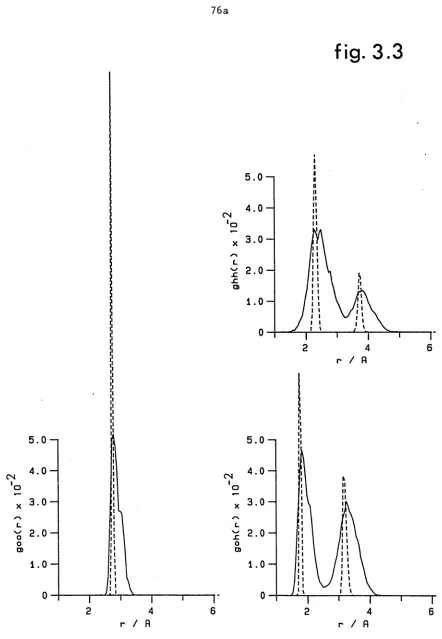
Atom - Atom pair distribution functions for water dimer. Solid line is the result of 4)0 2 averaging with the quantum random walk calculation. Dashed curve was obtained using classical Monte Carlo calculations at 10 K (Reimers (1982)). PAGE 76a
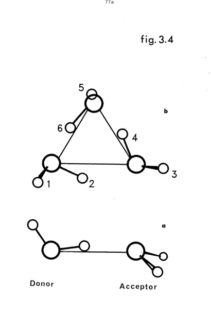
(a) Minimum energy geometry of water dimer, (b) Minimum energy
geometry of water trimer. PAGE 77a
3.6 Solid lines give the projections of the wave function of the water
dimer obtained from the random walk calculation onto the
intramolecular local coordinates. Dashed curves are the basis oscillator wave functions of water monomer. sb and sn are the bonded and non-bonded local coordinates on the donor molecule.
PAGE 80a
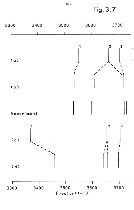
3.7 Comparison of basis oscillator frequencies obtained from (a)
random walk projection method and (c) "frozen field" local mode calculations. Spectra (b) and (d) show the influences of including couplings. Experimental spectrum was obtained by Coker, Miller and
Watts (1985). PAGE 81 a
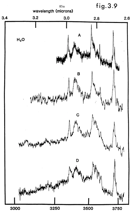
3.8 Experimental infrared predissociation spectra for H2O clusters at
high concentrations. Molecular beam compositions (% H2O in He) are
A: 17.5%, B: 24.2%, C: 36.3% and D: 52.1%. PAGE 84a
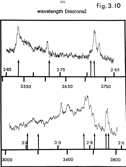
3.9 Low concentration water spectra corresponding to beam conditions;
A: 7.7%, B: 6.5%, C: 5.7% and D: 12.8%. PAGE 85a
3.10 Comparison of water dimer frequencies obtained from quantum
simulation projection method with experimental water cluster
3.11 Stick diagram comparing experimental and theoretical dimer and trimer IR absorption frequencies. The normal mode and local mode calculations use the RWKM potential of Reimers and Watts (1984b); random walk calculations combine the modified monomer surface described in the text with the RWK2 intermolecular potential of
Reimers, Watts and Klein (1981) (RWKM2) or with the earlier
surface of Watts (1977) (W77M2). PAGE 90a
3.12 Comparison of the RWK2 (solid line) and Watts (dashed line)
intermolecular potential surfaces (a) as a function of 0...0 distance minimizing energy at every separation, (b) as a function
of donor angle for fixed 0...0 distance and intramolecular
geometry and (c) as a function of acceptor angle for fixed 0...0
distance and intramolecular geometry. PAGE 91a
4.1 Relaxation of the energy estimate for a system of 32 Lennard Jones
helium atoms at a reduced density of p* = 0.4. The basic diffusion and birth death algorithm was used together with an initial fee geometry. Long range corrections have been included. N is the number of systems in the ensemble and the dashed and solid lines are respectively, the variational (Watts and Murphy (1970)) and
Green’s function Monte Carlo (Whitlock et al. (1979)) results.
32 helium atoms calculated with the importance sampling algorithm using different size time steps. These calculations employed an ensemble of 200 systems. The point with larger error bars was obtained using the unbiased random walk algorithm together with an ensemble of 1000 systems. The solid line gives tge GFMC value.
PAGE 110a
Solid lines are the extrapolated radial distribution functions for a system of 32 helium atoms obtained with the importance sampling algorithm using different size time steps. The points are the
results of GFMC calculations of Whitlock et al. PAGE 111a
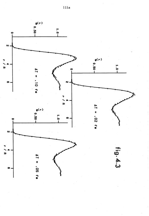
Extrapolation of the radial distribution function for He4 obtained from a Diffusion Monte Carlo calculation using 108 particles. The
short dashed line gives the distribution obtained from the
variational calculation, ip-p2, the long dashes are the diffusion Monte Carlo results averaged over the function ^7^, and the solid curve is the extrapolation. The points are the results of GFMC
calculations of Whitlock et al♦ PAGE 112a
Relaxation of the components of the energy of solid H 2 during importance sampled diffusion Monte Carlo calculations at various densities. The initial conditions were variational distributions. The short dash lines are the kinetic energies obtained by taking the difference between the total energies (solid lines) and the
4 . 6 E x t r a p o l a t i o n of t h e r a d i a l d i s t r i b u t i o n f u n c t i o n i n s o l i d H2 a t v a r i o u s d e n s i t i e s . S h o r t d a s h e s g i v e t h e g ( r ) ’ s o b t a i n e d from t h e
d i s t r i b u t i o n , l o n g d a s h e s from ip'pxp and t h e s o l i d c u r v e i s t h e e x t r a p o l a t e d ty2 r e s u l t . The p o t e n t i a l due t o Buck e t a l . ( 1983) i s a l s o p r e s e n t e d ( s o l i d c u r v e ) t o g e t h e r w i t h t h e Le nn a rd J o n e s (12 6) p o t e n t i a l f o r H2 ( d a s h e d c u r v e ) . PAGE 120a
5.1 The r i n g polymer s r e p r e s e n t i n g a two p a r t i c l e s y s t e m . The d i s c r e t e p a t h shown h e r e has 9 s e gment s and by c l o s i n g t h e r i n g a t d i f f e r e n t p o i n t s pr o p e r t i e s a t d i f f e r e n t t e m p e r a t u r e s can be
c a l c u l a t e d • PAGE 150a
C a l c u l a t e d and e x a c t e n e r g i e s of a h ar moni c o s c i l l a t o r (hco = 100 K) as a f u n c t i o n o f t e m p e r a t u r e . S o l i d l i n e s a r e e x a c t r e s u l t s o b t a i n e d from e q u a t i o n ( 6 . 2 ) . Dashed c u r v e s a r e t h e p r e d i c t i o n s of c l a s s i c a l t h e o r y . V a r i o u s c o l o u r e d symbols a r e t h e r e s u l t s of quantum Monte C a r l o c a l c u l a t i o n s u s i n g d i f f e r e n t i n i t i a l and f i n a l t e m p e r a t u r e s . C l a s s i c a l i n i t i a l d i s t r i b u t i o n s were u s e d .
C ol our b l a c k b l u e g r e e n r e d
T i n ( ° K ) 1000
500 100 100
T f i n ( ° K )
30 30 30 10
oscillator obtained at different temperatures along the random walk trajectory (T^n = 1000°K). Points are exact results obtained from equation (6.3). (b) Solid curves are the momentum distributions calculated at the same points along the trajectory. Crosses are the predictions of classical theory. PAGE 159a
Upper solid curve gives the temperature dependence of the total energy of the 0-H Morse oscillator obtained by summing over the analytic bound states. Lower solid and long dashed lines are respectively the potential and kinetic energies of the oscillator. Short dashed curves are classical results. Various coloured symbols are the results of quantum Monte Carlo calculations using different initial temperatures. Classical initial distributions were used.
Colour Tj n (°K)
black 10000
red 7500
blue 5000
PAGE 160a
Comparison of analytic results for the harmonic oscillator with values obtained from a quantum simulation using the exact position and momentum distributions at 100°K as the initial condition.
PAGE 162a
Same as Figure 6.3 except the improved high temperature approximation in Equation (6.9) is used to give the initial
6.6 (a) Comparison of the potential energy of low density neon gas at various temperatures obtained from quantum simulation (squares) with classical results (triangles). (b) Solid line gives the classical kinetic energy of neon gas and the squares are- the
results of quantum simulation. PAGE 167a
6.7 Pair distribution function in neon gas (p* = 0.0093) as a function of temperature. Solid curves are the results of quantum Monte Carlo simulations. Dashed curves give classical results and the points are taken from the work of Klemm and Storer (1972).
PAGE 168a
6.8 Momentum distributions in neon gas at various temperatures obtained from quantum simulation (solid curves) and classical
theory (dashed curves). PAGE 168b
6.9 Sample intramolecular distributions for the water dimer obtained from the quantum Monte Carlo calculations (solid curves) compared with the square of the ground state Morse oscillator eigenfunctions (dashed curves). With our resolution all the intramolecular distributions such as the bonded and non-bonded 0-H stretches were identical.
PAGE 172a
6.11 Comparison of classical and quantum intermolecular distributions for the water dimer at various temperatures. PAGE 173a
6.12 Comparison of classical and quantum intramolecular potential energy for the water dimer as a function of temperature. Dashed line is the ground state potential energy of a pair of isolated
monomers. PAGE 175a
6.13 Comparison of classical and quantum intermolecular potential energies for the water dimer as a function of temperature. Points at 100 °K are the results of Wallqvist and Berne (1985).
CHAPTER 1 AN OVERVIEW OF QUANTUM SIMULATION
Classical computer simulation methods have been used extensively to study both equilibrium and non-equilibrium behaviour of many body systems. The physical behaviour of a assembly of particles, however, is determined by quantum theory. Recently, a variety of quantum simulations methods have been developed and applied to studies of many body systems in which quantum effects are important. The algorithms can be divided into two categories: zero temperature methods for considering the individual quantum states of many body systems and non-zero temperature procedures in which a thermal distribution of quantum states is important. In this thesis we explore a stochastic numerical method which is useful for performing both zero and finite temperature calculations.
(1981))).
The basic "diffusion Monte Carlo" method which was first presented by Anderson (1975) and which is used throughout this thesis is developed and studied in detail in Chapter 2. The method involves using a "finite time step" approximation to solve a multidimensional diffusion equation. Results obtained using this approximation depend on the step size and in the limit as At ^ 0 exact values are obtained.
Diffusion Monte Carlo methods have been used mainly in studying electronic systems where the particle interactions vary relatively slowly with distance. Thus the finite time step approximation is expected to be valid. The most significant problem in using quantum Monte Carlo methods to study electronic systems is the treatment of identical particle statistics
(Kalos (1984)). In most of the electronic applications of the zero
temperature quantum Monte Carlo methods, approximate information about nodal surfaces in the Fermion wave function is used to provide boundary conditions for the random walks. Wave functions obtained from variational calculations are often used for this purpose. With the fixed node approximate methods (Reynolds et al. (1982)) the random walk results are dependent on the nodal surfaces used in the calculation. Methods for "relaxing" the nodes have been developed (Ceperley and Alder (1984)) and
essentially exact solutions which are antisymmetric with respect to
particle inerchange may be obtained.
In Chapter 2 we present an alternative procedure which does not require any prior knowledge of the nodal surfaces. Results of ab initio random walk calculations performed on the ground and excited states of small electronic systems using this approach are presented.
an a s s e mb l y o f Bosons s o e x a c t quantum Monte C a r l o c a l c u l a t i o n s can be p e r f o r m e d u s i n g Boltzmann s t a t i s t i c s . T h i s s i m p l i f i c a t i o n i s e x p l o i t e d i n C h a p t e r s 3 and 4 where we d i s c u s s t h e a p p l i c a t i o n of z e r o t e m p e r a t u r e quantum Monte C a r l o methods t o t h e s t u d y of t h e gr ound s t a t e p r o p e r t i e s of m o l e c u l a r c l u s t e r s and Boson s o l i d s and l i q u i d s .
R e c e n t l y t h e r e has been a g r e a t d e a l o f i n t e r e s t b o t h t h e o r e t i c a l l y and e x p e r i m e n t a l l y i n t h e s t u d y o f c l u s t e r s of atoms and m o l e c u l e s . With m o l e c u l a r beam t e c h n i q u e s , w e l l d e f i n e d c l u s t e r s can be p r e p a r e d i n a c o l l i s i o n f r e e e n v i r o m e n t . The i n t e r n a l d e g r e e s of freedom of c l u s t e r s p r o d u c e d by t h e s e methods a r e s t r o n g l y " c o o l e d " so e x p e r i m e n t a l r e s u l t s can be compared w i t h gr ound s t a t e c a l c u l a t i o n s . I n C h a p t e r 3 we d e s c r i b e t h e r e s u l t of some gr ound s t a t e quantum Monte C a r l o c a l c u l a t i o n s p e r f o r m e d on s m a l l c l u s t e r s of w a t e r m o l e c u l e s . A method f o r s t u d y i n g t h e i n t r a m o l e c u l a r v i b r a t i o n s of m o l e c u l e s i n c l u s t e r s u s i n g t h e wave f u n c t i o n o b t a i n e d from a g round s t a t e quantum Monte C a r l o c a l c u l a t i o n i s p r e s e n t e d . C a l c u l a t e d v i b r a t i o n a l s p e c t r a a r e compared w i t h m o l e c u l a r beam r e s u l t s . The i n p u t t o t h e s e c a l c u l a t i o n s i s a p o t e n t i a l s u r f a c e and we d e m o n s t r a t e t h a t c om pa ri ng t h e v i b r a t i o n a l s p e c t r a o b t a i n e d from gr ound s t a t e quantum Monte C a r l o c a l c u l a t i o n s w i t h t h e r e s u l t s of m o l e c u l a r beam e x p e r i m e n t s p r o v i d e s a s e n s i t i v e t e s t f o r t h e p o t e n t i a l s u r f a c e .
(1972)). These methods provide an upper bound on the energy of the system and hence approximate ground state thermodynamic properties are obtained. Thus comparison with experiment is ambiguous. With the quantum Monte Carlo methods, however, different interaction potentials can be reliably tested
(Whitlock et al. (1980)].
In Chapter 4 we consider applying the diffusion Monte Carlo method to study bulk phase quantum systems with strongly repulsive interactions. The basic algorithm is not useful for these studies and improvements in the efficiency and accuracy of the method are necessary. Importance sampling techniques, in which approximate many body wave functions are used to guide the diffusion Monte Carlo procedure to sample the more important regions of configuration space, greatly reduce the statistical fluctuations during the
simulation. With these improvements efficient bulk phase quantum
calculations can be performed.
The finite time step approximation is expected to be most severe in dense systems with strongly repulsive interactions. By using different time steps in bulk phase calculations the significance of this approximation is considered. At higher densities smaller time steps are used and over the range of step sizes considered in our work, little time step dependence is observed.
We have used the spherical part of a semiempirical intermolecular pair
potential due to Buck et al. (1983) in diffusion Monte Carlo calculations
As m e n t i o n e d e a r l i e r , t h e quantum Monte C a r l o methods p r o v i d e a g e n e r a l means f o r s o l v i n g m u l t i d i m e n s i o n a l d i f f u s i o n e q u a t i o n s . I n t h e c a s e o f t h e z e r o t e m p e r a t u r e me t h o d s , s t a t i o n a r y s o l u t i o n s of t h e S c h r ö d i n g e r e q u a t i o n a r e o b t a i n e d . Quantum Monte C a r l o methods can a l s o be u s ed t o g i v e " t i m e " e v o l v i n g s o l u t i o n s of d i f f u s i o n e q u a t i o n s . The b e h a v i o u r o f a s y st e m a t n o n - z e r o t e m p e r a t u r e s i s g o v er n ed by t h e d e n s i t y m a t r i x which e v o l v e s as a f u n c t i o n of t h e i n v e r s e t e m p e r a t u r e , ß = V k g T , a c c o r d i n g t o a d i f f u s i o n e q u a t i o n known as t h e Bloch e q u a t i o n . The n o n - z e r o t e m p e r a t u r e quantum Monte C a r l o p r o c e d u r e d e s c r i b e d i n C h a p t e r 5 u s e s t h e methods employed w i t h t h e z e r o t e m p e r a t u r e t e c h n i q u e s t o s o l v e t h e Bloch e q u a t i o n . From t h e e v o l u t i o n of t h e s o l u t i o n , i n f o r m a t i o n a t d i f f e r e n t t e m p e r a t u r e s i s o b t a i n e d .
The f o r m u l a t i o n o f t h e n o n - z e r o t e m p e r a t u r e method p r e s e n t e d h e r e i s d i f f e r e n t from t h e p a t h i n t e g r a l Monte C a r l o p r o c e d u r e s which have been d e v e l o p e d r e c e n t l y b u t t h e methods a r e e q u i v a l e n t . F i n i t e t e m p e r a t u r e p a t h i n t e g r a l t e c h n i q u e s have been u sed t o s t u d y a v a r i e t y of i n t e r e s t i n g p r o b l e m s . The p r o p e r t i e s of l i q u i d ^He ( P o l l o c k and C e p e r l e y ( 1 9 8 4 ) ) and Neon ( T h i r u m a l a i e t a l . ( 1 9 8 4 ) ) a t n o n - z e r o t e m p e r a t u r e s have been e x p l o r e d . S o l v a t i o n o f e l e c t r o n s i n f u s e d s a l t s ( P a r r i n e l l o and Rahman ( 1 9 8 4 ) ) , t h e p h y s i c a l p r o p e r t i e s of c l u s t e r s of Argon atoms (Freeman and D o l l ( 1 9 8 5 ) ) , s o l v a t i o n o f H atoms and muonium i n c l a s s i c a l w a t e r (öe Raedt e t a l . ( 1 9 8 4 ) ) as w e l l as t h e c a l c u l a t i o n of e l e c t r o n i c and v i b r a t i o n a l s p e c t r a o f m o l e c u l e s ( T h i r u m a l a i and Berne ( 1 9 8 3 ) , ( 1 9 8 4 ) ) a r e some of t h e p r o bl e m s which have been e x p l o r e d r e c e n t l y u s i n g p a t h i n t e g r a l m e t h o d s .
the distribution through ß and the Bloch equation is simulated. This approach provides a means of obtaining results at a number of different
temperatures during a single calculation. Information about quantum
position and momentum distributions may be obtained using this approach as well as thermodynamic data.
In Chapter 6 the use of the non-zero temperature diffusion Monte Carlo
method is demonstrated by considering some representative problems,
including the one dimensional Morse and harmonic oscillators, quantum effects in neon gas and finally the quantum behaviour of the water dimer as a function of temperature. More accurate high temperature approximations must be used as the initial condition for the intramolecular vibrations of
the cluster but classical results may be employed to give initial
conditions for the intermolecular degrees of freedom.
CHAPTER 2 BASIC QUANTUM MONTE CARLO, DEVELOPMENT AND SIMPLE APPLICATIONS
Introduction
In this chapter the quantum random walk method is developed and applied to some simple illustrative problems. The methods described are employed in subsequent chapters to study some important many body quantum problems.
Chapter 2 is organised as follows: After a brief description of basic quantum theory we consider the analogy between the Schrödinger equation and a diffusion process modified by chemical reaction. The analogy is used to develop a numerical model of the Schrödinger equation based on a "short time" approximation. The method produces an ensemble distributed according to the wave function and the number of systems in the ensemble decays at a rate proportional to the eigenvalue.
In Section 2.) the question of symmetry and the generation of nodal surfaces in the wave function is considered. A feedback mechanism for maintaining a stable ensemble is discussed. The stabilizing method provides an efficient means for estimating the eigenvalue but it allows only the ground state distribution to be sampled. Next, a procedure for forcing the distribution to remain orthogonal to the ground state is described. With this technique a stable excited state distribution can be sampled. After studying the excited vibrational states of molecular hydrogen we consider extending the approach to many dimensions, using the S and P states of the hydrogen atom as an example.
of v a r i o u s o p e r a t o r s from a quantum random walk c a l c u l a t i o n . We a l s o c o n s i d e r i m p o r t a n c e s a m p l i n g methods which a r e used t o improve t h e e f f i c i e n c y o f quantum Monte C a r l o c a l c u l a t i o n s .
F i n a l l y i n S e c t i o n H.) we c o n s i d e r t h e q u e s t i o n of i d e n t i c a l p a r t i c l e s t a t i s t i c s . A f t e r d i s c u s s i o n of some t e c h n i q u e s which have been u sed f o r t r e a t i n g Fermi s y s t e m s we c o n s i d e r g e n e r a l i s i n g t h e method f o r g e n e r a t i n g n o d a l s u r f a c e s d e s c r i b e d i n S e c t i o n 2 . ) so t h a t an a n t i s y m m e t r i c d i s t r i b u t i o n i s o b t a i n e d . With t h i s p r o c e d u r e s y s t e m s c o n t a i n i n g a few f e r m i o n s can be s i m u l a t e d . As e xa m p l es , d i f f e r e n t s p i n s t a t e s of a t o m i c h e l i u m and l i t h i u m a r e mod e le d.
1 . ) The B a s i c Quantum Monte C a r l o A l g o r i t h m
a) Formal P r e l i m i n a r i e s
I n quantum m e c h a n i c s , t h e b e h a v i o u r of a s ys te m i s d e t e r m i n e d by t h e wave f u n c t i o n \Jj(r_, t ) . For a n o n - r e l a t i v i s t i c s y s t e m , \ | i ( r , t ) obeys t h e S c h r ö d i n g e r e q u a t i o n ( Mer zbache r ( 1 9 7 0 ) ) which t a k e s t h e f o l l o w i n g form
ifi3_ \ K r , t ) = H iIj ( r , t) ( 2 . 1 )
at
N _ 2 2
= I
— vk I| j( r, t) + ( v ( r ) - V r e f ) ^ ( r , t ) k 2mk/s
There are an infinite number of solutions to equation (2.1). The set of
solutions which are products of separate functions of time and space
ij;(r,t) = f(t) c|>(r) (2.2)
are of particular physical importance. Substituting (2.2) into equation
(2.1) and separating variables we find that
and
f (t)
(E V r e f)
Vk <J)(r) + ( v ( r ) - V r e f ) ( E - V r e f ) <)>(r)
(2.3)
(2.H)
Where (E-Vref) is the separation constant.
Equation (2.4), the time independent Schrödinger equation, is an
eigenvalue equation
H <|>(r) = (E-Vr e f ) (j>(r)
Since H is a hermitian operator its eigenvalues, (E-Vre f), are real. Thus
f(t) is a purely oscillatory function of time.
For particular solutions of the form
\|<(r, t ) = e " it/1,‘(E" Vr’ef ) ^(r) (2.5)
the probability density, ij;*(r,t ) 14(r ,t ), is independent of time. For this
reason such solutions are said to represent "stationary states" of the
s y s t e m .
In a stationary state the expectation value of a time independent
physical property represented by an operator, A, depends only on the time
<A> ijj*(r_,t) Ai[»(r,t) dr
J
4>*(r) A<t>(rO d r (2.6)G e n e r a l s o l u t i o n s of t h e S c h r ö d i n g e r e q u a t i o n can be c o n s t r u c t e d by s u p e r p o s i t i o n o f p a r t i c u l a r s t a t i o n a r y s o l u t i o n s . Thus, i f t h e ti me i n d e p e n d e n t S c h r ö d i n g e r e q u a t i o n y i e l d s a s e t of e i g e n f u n c t i o n s 4>n ( r ) which a r e c o m p l e t e i n t h e s e n s e t h a t any i n i t i a l s t a t e , \Jj(r_,0), may be expanded i n t e r m s o f them
t|j(r, 0 ) = I an c{>n ( r ) ( 2 . 7 )
n
t h e n t h e s o l u t i o n f o r a l l l a t e r t i m e s w i l l be o f t h e form
i |»(r, t) = Iane ~ 1 (En~vr e f 5 ^ ( r ) ( 2 . 8 ) n
I n t h i s c h a p t e r we d e s c r i b e a c o m p u t a t i o n a l method f o r s o l v i n g t h e e i g e n v a l u e problem p r e s e n t e d i n t h e t i me i n d e p e n d e n t S c h r ö d i n g e r e q u a t i o n . The p r o c e d u r e i n v o l v e s s i m u l a t i n g t h e t i m e d e p e n d e n t S c h r ö d i n g e r e q u a t i o n by making u s e o f t h e a n a l o g y bet ween ( 2 . 1 ) and an e q u a t i o n which d e s c r i b e s a combined d i f f u s i o n and c h e m i c a l r e a c t i o n p r o c e s s . I n t h i s s e c t i o n we s h a l l p r e s e n t t h e b a s i c t e c h n i q u e u s ed t o o b t a i n ground s t a t e p r o p e r t i e s . The q u e s t i o n s of i d e n t i c a l p a r t i c l e s t a t i s t i c s and wave f u n c t i o n symmetry w i l l be c o n s i d e r e d i n l a t e r s e c t i o n s .
b ) The D i f f u s i o n E q u a t i o n Analogy, a N umer ic al Model of t h e S c h r ö d i n g e r E q u a t i o n
D e f i n i n g t h e " i m a g i n a r y t ime" v a r i a b l e x = i t / h e n a b l e s t h e wave e q u a t i o n g i v e n i n ( 2 . 1 ) t o be t r a n s f o r m e d i n t o t h e f o l l o w i n g
| i ( L * T) = I V ^ ( r , x ) - (V( r ) - V r e f )t>( r_, x) ( 2 . 9 )
the diffusion of a concentration profile through a fluid. The second term resembles an equation which models exponential growth and decay or a first order chemical rate process. Thus the Schrödinger equation in imaginary time is analogous to an equation describing diffusion which is modified by a chemical reaction whose rate changes with position. In this analogy the wave function is treated as the density of diffusers.
In the absence of the "birth/death" term, the solution of the diffusion part of equation (2.9) with the initial condition
ijj(r,t=0) = <5(r-r0)
is well known
i | > ( r , x)
N
,
-<D<-
iW
2
/
i,
dn 2 e
k
kT (2.1 0)
Here rk is the position of particle k in three dimensional space and Dk is the diffusion coefficient of the particle and depends on its mass
Dk = /2mk
By interpreting the wave function as a density, equation (2.10) is treated as the distribution function for an ensemble of free particle systems moving in imaginary time. The evolution of the ensemble can be modeled on a computer. First a set of systems is established at r0 . In a time At, each particle should sample a three dimensional Gaussian distribution centred on
rko with variance Axk = (2DkAx)2. The distribution may be sampled
en s emb l e d i s t r i b u t i o n w i l l s p r e a d o u t as t h e wave f u n c t i o n g i v e n i n e q u a t i o n ( 2 . 1 0 ) .
A n u m e r i c a l model f o r s i m u l a t i n g t h e e f f e c t s of t h e p o t e n t i a l te rm i n e q u a t i o n ( 2 . 9 ) can be d e v i s e d u s i n g t h e a n a l o g y bet ween t h i s te rm and a p h e n o m e n o l o g i c a l r a t e e q u a t i o n . The model i n v o l v e s r e p l i c a t i n g o r removi ng s y s t e m s from an ensembl e d e p e n d i n g on t h e p o t e n t i a l e n e r g y .
I g n o r i n g t h e d i f f u s i o n t e r m , e q u a t i o n ( 2 . 9 ) g i v e s t h a t t h e a m p l i t u d e of t h e wave f u n c t i o n a t some p o i n t r c ha n g e s i n t i m e as f o l l o w s
- ( V ( r ) - V r e f ) * ( r )
R e a r r a n g i n g and i n t e g r a t i n g f o r a f i n i t e t i m e , At, we have
ip-*-Aip x+Ax
1 ? = - J ( V- V r e f )dT
Ip ^ X
Thus t h e change i n a m p l i t u d e o f t h e wave f u n c t i o n a t r d u r i n g Ax i s
Aip(r) = i p ( r ) ( e " (V(- ) _Vref)AT- 1 )
C o n s e q u e n t l y a t t i me x + Ax we have
^(x+Ax) = ^ (t) + Alj,
(2.1 1)
= e~ (V vr e f ) Ax
The p o p u l a t i o n of t h e e ns embl e can be made t o grow or deca y a c c o r d i n g t o e q u a t i o n ( 2 . 1 1 ) by d e f i n i n g t h e b i r t h p r o b a b i l i t y as
Pb = e' ( v" vr e f ) At-1 ( 2 . 1 2 )
parts.
Pb = int(Pb ) + frac (Pb )
The necessary births can be accomplished by producing int(Pb ) replicas together with an extra replica included with a probability frac(Pb ). When
the energy of a system is such that V > Vref , there is a probability
pd = “pb that the system will "die” and be removed from the ensemble.
The numerical methods for treating the separate terms in the
Schrödinger equation which were discussed above are exact independent of
the size of the time step. Anderson (1975, 1976) has presented an
approximate procedure for simulating the Schrödinger equation which
involves combining the diffusion and birth/death processes by making a
short time approximation. Thus it is assumed that the potential is
approximately constant over the short distances through which systems move as a result of diffusion for a finite time At.
The idea of studying quantum problems using the analogy between the time dependent Schrödinger equation and a diffusion and birth/death process has been attributed to Fermi (Metropolis and Ulam (1949)). In the 1950’s several workers discussed various Monte Carlo methods based on this idea
and Anderson (1975) presents a summary of these early references. Most of
summarised as follows:
1) Establish an ensemble of systems in some initial distribution.
2) Increament time by At and allow each ensemble member to diffuse by
giving its particles random cartesian displacements, the
components being chosen from Gaussian distributions of appropriate width.
3
)
Calculate the potential energy of each displaced system and,depending on this value, allow the system to replicate or "die".
Repeating steps 2) and 3
)
enables the imaginary time evolution of theinitial ensemble to be followed and, if a sufficiently small time step is used, the ensemble motion models the evolution of the wave function.
The initial distribution can be expanded in terms of the eigenfunctions of the Hamiltonian and the time evolution is thus determined by equation
(2.8), which can be written in imaginary time as
<Kr,x) =
I
ane (En~vref)t ^ ( r ) (2 .13)n
As t 00 the sum will be dominated by the lowest energy eigenstate
contained in the initial expansion. Thus in the long time limit, the
simulation algorithm summarised above will produce an ensemble of systems distributed in space according to the eigenstate, <j)0 and since
<l«(r,T) = a0e'(E°_Vref)T *0 (r) <2.1 M)
the asymptotic population decay rate will give an estimate of the
eigenvalue E0 .
70
X
o
3
ro
J_ _ _ _ _ _ I_ _ _ _ _ _ I
ro
( N )
6
° I
CO ^ CJI
X o
CD O
ro
■
cr
f
i
g
dimensional harmonic oscillator. Parameters are chosen to model a proton in a harmonic well V(x) = £kx2 with force constant k = 100 KA"^. The initial condition was an ensemble of 100 systems, all with zero displacement. Figure 2.1a shows the evolution of this ensemble in imaginary time. Here, histograms of the ensemble displacements have been accumulated at various times along the trajectory. The curves are the result of averaging over 100 such trajectories all having the same initial condition. At short times the ensemble distribution undergoes some initial spreading following which a stable Gaussian distribution of constant width is obtained. The amplitude of the distribution decays along the trajectory. In Figure 2.1b we plot the logarithm of the ensemble population as a function of time. After some
transient behaviour, associated with the spreading of the initial
distribution, a constant exponential decay rate is established. The
asymptotic slope of this line gives the ground state energy of the oscillator.
There are several problems with the simple minded algorithm described in this section. The birth/death step causes exponential growth or decay of the ensemble population. Thus at long times, if the population is decaying there will be problems with small sample sizes while if population growth
occurs the available computer storage will be exceeded. Time step
must be d e v e l o p e d .
2. ) E x t e n s i o n of t h e B a s i c A l g o r i t h m
a) Wave F u n c t i o n Symmetry
The Monte C a r l o method f o r m o d e l i n g t h e S c h r ö d i n g e r e q u a t i o n d i s c u s s e d i n S e c t i o n 1 . ) d e a l t o n l y w i t h s i m u l a t i n g t e r m s i n t h e H a m i l t o n i a n . So f a r we have s a i d n o t h i n g a b o u t bo un da ry c o n d i t i o n s or wave f u n c t i o n symmetry. We c o n f i n e o u r s e l v e s t o c o n s i d e r i n g o n l y r e a l wave f u n c t i o n s . I n g e n e r a l s u ch wave f u n c t i o n s have p o s i t i v e and n e g a t i v e r e g i o n s . C o n s e q u e n t l y a t e c h n i q u e f o r g e n e r a t i n g n o d a l s u r f a c e s i n t h e s ampl ed d i s t r i b u t i o n must be d e v i s e d .
Anderson and F r e i h a u t (1979) d i s c u s s e d a random walk method f o r s a m p l i n g t h e d i f f e r e n c e , 6 = ip— , b e t we e n t h e gr ound s t a t e wave f u n c t i o n \\>
and a t r i a l f u n c t i o n ipp. I n g e n e r a l t h e f u n c t i o n 6 w i l l have nod es and t h e i r random walk i n v o l v e s p o s i t i v e and n e g a t i v e s y s t e m s which c a n c e l when o p p o s i t e s i g n e d s y s t e m s e n t e r e d t h e same r e g i o n o f s p a c e . The method was a p p l i e d t o s e v e r a l one d i m e n s i o n a l p r o bl e ms and when us ed i t e r a t i v e l y gave a s e r i e s of s u c c e s s i v e c o r r e c t i o n s t o t h e t r i a l f u n c t i o n which i mpr oved t h e e f f i c i e n c y and a c c u r a c y of gr ou nd s t a t e c a l c u l a t i o n s .
X
o
3
ro
( N )
6
oI
o o
o
ro
■
fNJ
O’
f
1g
walkers climbed up the walls of the potential surface. When opposite signed systems are introduced and annihilation occurs, the boundary conditions on the wave function also give the possibility for "death".
Figure 2.2 again shows results from a quantum simulation of a harmonic oscillator. Now however the initial condition was 50 positive random walkers placed at +a and an equal number of negative systems at -a. The annihilation step was included at the end of each time step after the systems had diffused and replicated. Two systems of opposite sign were allowed to annihilate if they were separated by a distance less than some small value. From the figure we see that the ensemble distribution propagates to the first excited state wave function after some transient behaviour. Figure 2.2b demonstrates that the asymptotic population decay rate gives the first excited state eigenvalue. Later in this section we consider extending the annhilation procedure to more than one dimension and in Section 4.) we discuss the question of annihilation of systems with many identical particles.
b) Producing a Stable Ensemble
From equation (2.14) a stable ground state population may be obtained by setting the value of the reference in the energy scale, Vref, equal to the ground state energy E0 . To use this method requires prior knowledge of the ground state energy. We might consider setting Vref to some guess at E0 and monitoring the population as the simulation proceeds. Adjusting Vref so that on average the population neither grows nor decays gives a means of estimating E0 .
with average population N c . At the end of each time step a new value for Vref is chosen according to the following expression
W t+ At - <v>t -
“(NT-NC)
(2.15)
Here N x is the instantaneous total number of systems in the ensemble and <V > T is the average potential energy. The parameter a is a positive energy which controls the size of the population fluctuations. As i->“ the spatial distribution will be approximately constant and <V>T will not change appreciably with time. Choosing Vrefx+Ax according to (2.15), gives an energy reference which is appropriately larger or smaller than <V>T so that on average the births or deaths in the next time step will correct any discrepancey between N T and N c . If the parameter a is too large, the feed back mechanism may become unstable.
An understanding of the influence of the feed back mechanism described above can be obtained by expanding the distribution in terms of the eigenfunctions {4>n }
ip(r»x) =
1
an (i) ^n^H) (2.16) nHere the exponential decay factors appearing in equation (2.13) have been replaced by time varying expansion coefficients an (i). When Vrep is varied with time the coefficients no longer exhibit decoupled exponential decay.
To proceed we consider the Schrödinger equation in which the reference energy varies
f~(-’
t) - [jjjV - (v(r) - vref
(t) )] iKr.-t)
(2.17)
o v e r a l l s p a c e we f i n d t h a t t h e c o e f f i c i e n t s s a t i s f y t h e f o l l o w i n g d i f f e r e n t i a l e q u a t i o n s
- 5 7 = - ( E n -Vr e f ( T ) ) a n ( T) ( 2 . 1 8 )
Thes e e q u a t i o n s a r e c o u p l e d t h r o u g h t h e f u n c t i o n Vr e p ( x ) . The e x p l i c i t form o f t h e c o u p l i n g can be foun d by w r i t i n g t h e e x p r e s s i o n f o r t h e Vr e f a d j u s t m e n t ( e q u a t i o n ( 2 . 1 5 ) ) i n t e r m s of t h e e i g e n f u n c t i o n e x p a n s i o n .
When o p p o s i t e s i g n e d s y s t e m s a n n i h i l a t e one a n o t h e r , t h e t o t a l number o f s y s t e m s i n t h e e ns emb le a t t i m e t i s p r o p o r t i o n a l t o t h e a r e a und er t h e f u n c t i o n |ijj(r, t)| t h u s we can w r i t e
Nx = { | I a n ( t) M i l )
I
dL nS i m i l a r l y , t h e a v e r a g e of t h e p o t e n t i a l e n e r gy a t t i me t can be w r i t t e n as
j 1 1 a n ( t) <J>n ( £ ) | V ( r ) d r <V>T = n_____________________
{ | I
a n ( t) cj)n ( r ) | drn
S u b s t i t i n g t h e s e r e s u l t s i n t o ( 2 . 1 5 ) g i v e s t h e f o l l o w i n g e x p r e s s i o n f o r t h e t i m e e v o l v i n g e n e r g y r e f e r e n c e
J
I I
a n<T)M il) I
V ( r ) d r ( 2 . 1 9 ) V r e f ( l ) " — f -- - - “ a [ J | I a n ( t) ^ n ( £ ) | d H “ N c ]J
I 5! a n (
t
) <J)n ( r ) | d L
n
n
considering the behaviour of the solutions of (2.18) and (2.19) for a problem where the eigenvalues and eigenfunctions are known.
Harmonic oscillator eigenvalues and eigenfunctions have been used, and equations (2.18) and (2.19) solved numerically to give the solutions shown in Figure 2.3a. The initial distribution was dominated by the first excited state eigenfunction and contained small components of the ground and other excited states. Through the nature of the couplings introduced in Vref(i), the lowest lying state contained in the initial distribution is amplified at the expense of the other states. Further, at long times the amplitude of the lowest energy initial state attains a constant value and the excited state contributions decay to zero.
Behaviour similar to this can be observed in a random walk simulation using the Vref adjusting algorithm. The wave function is represented by an ensemble of positive and negative systems and can be written in the following form
4>(H»
t)
= I 6(r-rp(i)) - I <5(r-r^j
( t))
(2.20)p m
Here rp (x) and r ^ x ) , respectively, give the positions of positive and negative systems at time x. When xp(jn, x) is written in terms eigenfunction expansion in (2.16), the expansion coefficients are obtained from the overlap between ^ and the eigenfunctions so that
an (x) =
j
i> (r, x)~ I ^n^-Hp^T-)) “ I ^n^Urn^T))
p m
(
2.
21)
5 0 0 10 0 0 T im e x 1 0 * * -1 5 e
C 1 ) u d
I ( 1 ) u d
0 * ♦ 1
«9
ro 4^. o)
Equation (2.21) can be used to resolve the ensemble distribution into its eigenfunction components. Figure 2.3b shows the evolution of the first five expansion coefficients calculated, using equation (2.21), during a simulation of the harmonic oscillator in which Vref was adjusted according to equation (2.15). The initial condition was an ensemble of fifty positive systems at +a and fifty negative systems at -a. An annihilation step was included in the algorithm. The ensemble is dominated by the ground state distribution at long times.
It is interesting to note that the initial distribution for the random walk calculation considered above contains no component of the ground state. If the system of differential equations (2.18) and (2.19) is solved with this initial condition the results shown in Figure 2.3c are obtained. The first excited state establishes itself with constant amplitude while the other excited states decay. Throughout the calculation the ground state
remains with zero amplitude. The qualitative difference between the
behaviour of the solutions of equations (2.18), (2.19) and the results of the simulation is due to the fact that the equations do not include the statistical fluctuations which occur in the simulation algorithm. Thus in Figure 2.3b we see a component of the ground state enter the ensemble distribution through statistical noise which is amplified and dominates the asymptotic ensemble distribution.
c) O r t h o g o n a l F i l t e r i n g and S t a b l e E x c i t e d S t a t e D i s t r i b u t i o n s
I n o r d e r t o us e t h e Vr e f a d j u s t i n g a l g o r i t h m t o o b t a i n a s t a b l e e x c i t e d s t a t e d i s t r i b u t i o n we need t o d e v i s e a scheme t o remove g r ound s t a t e components which may b u i l d up as a r e s u l t of s t a t i s t i c a l n o i s e . From e q u a t i o n ( 2 . 2 1 ) t h e o v e r l a p bet ween t h e e ns embl e d i s t r i b u t i o n and t h e gr ound s t a t e wave f u n c t i o n i s g i v e n by
a 0 ( = I 4> o ( r p ( x ) ) “
I
cf>0 (i j t i( t) ) ( 2 . 2 2 )p m
By f o r c i n g a 0 (x) t o r e m a i n a p p r o x i m a t e l y z e r o , g r ou nd s t a t e components can be f i l t e r e d from t h e d i s t r i b u t i o n . To u s e e q u a t i o n ( 2 . 2 2 ) , t h e g r ou nd s t a t e wave f u n c t i o n must be known i n a d v a n c e .
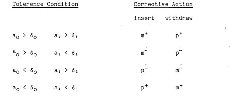
One p r o c e d u r e t h a t e n s u r e s o r t h o g o n a l i t y i s summarised as f o l l o w s : At t h e end o f each t i m e s t e p we c a l c u l a t e t h e o v e r l a p w i t h t h e g r ound s t a t e . I f a 0 ( i ) i s g r e a t e r t h a n some t o l e r e n c e 6 t h e n t h e o v e r l a p must be r e d u c e d . By removi ng a p o s i t i v e s ys te m o r i n t r o d u c i n g a n e g a t i v e s y s t e m , a 0 (x) can be changed a p p r o p r i a t e l y . I f n e c e s s a r y t h e o v e r l a p can be i n c r e a s e d i n a s i m i l a r f a s h i o n . The t o t a l number of s y s t e m s s h o u l d n o t be d i r e c t l y a l t e r e d by t h e o r t h o g o n a l i s a t i o n s t e p , r a t h e r , o n l y t h e s h ap e of t h e d i s t r i b u t i o n s h o u l d be c ha n g e d . I n t h i s way t h e r a t e of change of t h e p o p u l a t i o n i s n o t d i r e c t l y i n f l u e n c e d by t h e o r t h o g o n a l i z a t i o n . By r e p l i c a t i n g and removi ng o p p o s i t e s i g n e d s y s t e m s t h e r e l a t i v e numbers of p o s i t i v e and n e g a t i v e components can be a d j u s t e d so t h a t a 0 ( x) i s f o r c e d t o f l u c t u a t e ar ou nd z e r o .
5
0
0
1
0
0
0
T
im
e
x
1
0
*
*
-1
5
s
( 1 ) U d
ro
cn
oo
o
o
o
o
o
1
0
initial ensemble consisting of fifty negative systems at both +a and -a and one hundred positive systems at the origin was used. This condition resembles the second excited state of the oscillator. We see from the figure that there is also an initial component of the fourth excited state. As time is advanced the contributions from <j>2 and $4 decay and the first excited state component grows and stabilizes, dominating the asymptotic distribution. The ground state noise level does not build up during the calculation indicating that the orthogonalization procedure effectively filters ground state components from the ensemble. There are, however, significant components of the higher excited states which do not decay to zero and which perturb the stable excited state distribution.
The procedure discussed above can be used to simulate higher excited states. With such calculations, all the lower energy eigenfunctions must be known and the ensemble distribution is held orthogonal to these states. As an example consider the second excited state so there are two orthogonality conditions to be satisfied.
a0 (i) = I 4>0 tllp(T)) ~ l o (jjn(T)) = 0 (2.23)
p m
ai ( t) = I <f>i (llp( t)
)
“I
<h (ijnC t)) = 0 (2.24)Table 2.1 Procedure for Maintaining Orthogonality to the ground and first exited states
Tolerence Condition
a0 ^ <$o a i > <51
ao ^ ^o ai < 6 i
a 0 < <5o a i > 6 i
a0 < <50 ai < 5 i
Corrective Action
insert withdraw
+ _ +
m p
m~ p~
P
P +
m
In the table, the notation m + represents a negative system which is in a
region of space where the value of the first excited state eigenfunction is
positive. Thus for example, if a0 > 60 and the excited state overlap
a x > 6 1, the action which will correct these discrepancies and leave the
total population unaltered is to introduce an extra negative system and
withdraw a positive system. Both changes should occur in regions where cj>-|
is positive. An alternative to the replication and removal of opposite
signed systems is to change the sign of a single system. We have used this
alternative in applications only when there are no systems available for
replication in the appropriate region of space.
The excited state method detailed in this section has been used to
simulated the first few vibrational eigenstates of the H 2 molecule. The
vibrational potential surface presented by Kolos and Wolniewicz (1975) was
used. A ground state calculation was first performed and a histogram of the
ensemble distribution accumulated. Fitting a piece wise cubic polynomial
through this data gave a form for the ground state wave function which
could be used for the orthogonalization step in the excited state
[image:46.552.97.501.144.328.2]V
C
r)
x
1
0
*
*
4
f i g . 2 . 5
- 3 . 0 - 1
4 . 0
5 . 0
--
6 . 0
0 . 5 0 1 . 0
vibrational states obtained in this way are presented in Figure 2.5. In Table 2.2 we give the corresponding eigenvalues which were calculated from the average value of Vref required to hold the population approximately constant. The ground state energy agrees with the result of Kolos and Wolniewicz and the excited state energies are slightly too high. The
discrepancy probably results because of higher eigenstate impurities
(Figure 2.4) which may arise through noise introduced by the
orthogonalization procedure.
Table 2.2. Vibrational Energies
V Random Walk
0 -5.19
1 -4.58
2 -3.97
of the H2 Molecule (in 10^°K)
Kolos and Wolniewcz (1975)
-5.20 -4.60
-4.03
d ) System Annihilation in Many Dimensions
of members would be required otherwise the opposite signed systems could never find one another, no annhilations would occur, and two opposite signed ground state distributions would result. If the members of the ensemble occupy a non-infinitessimal volume of the configuration space, a finite ensemble can be used.
The simplest means for giving the systems a finite size is to use a 3N dimensional rectangular grid to define the configuration space. Instead of being represented by a multidimensional delta distribution, each system now occupies a small hypercube. Results obtained using this procedure will depend on the size of grid and on the number of systems in the ensemble. If the grid were too fine and the ensemble population to small to fill the space then opposite signed systems could easily avoid one another and positive and negative ground state distributions would again result. The problem can be remedied by increasing the number of systems in the ensemble, which increases the computational effort involved with the calculation. Alternatively, we may use a coarser spatial grid. Adopting the latter measure means that the resolution of the spatial features of the wave function, such as the nodal surfaces, will be poorer and the accuracy of the eigenvalue effected. Ideally, the number of systems in the ensemble may be increased till a particular spatial grid becomes "saturated". Beyond this point, any increase in the number of systems will have no effect on the calculation and the results will depend only on the spatial resolution.
a n a l o g o u s to the grid size. The nodes of a wave f u n c t i o n are gen e r a l y
cu r v e d s u faces in h y perspace. U s i n g a local G a u s s i a n d e nsity s h o u l d p r ovide
a b etter r e p r e s e n t a t i o n of these s u r f a c e s than the r e c t a n g u l a r grid. Thus
fewer s ystems o c c u p y i n g l arger volumes s h o u l d give co m p a r a b l e accuracy.
W h e n r e p r e s e n t e d by a G a u s s i a n d e n s i t y profile, the s patial extent of
s y s t e m i is g iven by
W h e n r e p r e s e n t e d as delta d i s t r i b u t i o n s the a n n i h i l a t i o n p r o b a b i l i t y for o p p o s i t e si g n e d s ystems was zero if their r e s p e c t i v e i n f i n i t e s s i m a l v o lume
e l e m e n t s did not o v e r l a p and one if there was any o v e r l a p at all. A
c o n s i s t e n t d e f i n i t i o n for the a n n i h i l a t i o n p r o b a b i l i t y is thus
For sy s t e m with G a u s s i a n d e n s i t y the a n n i h i l a t i o n p r o b a b i l i t y b e c o m e s
An effi c i e n t sc h e m e for i m p l e m e n t i n g the a n n i h i l a t i o n s tep involves
P i ( r ) (ä)3N/2 e- a ( r - r i )2 (2.25)
The o v e r l a p of the d e n s i t y p r ofiles for sys t e m s i and j is then
(2 .26)
00
pa ( | r i - r j | ) = 2 { S(t)dt
I
Li
I
(2.27)
(2.28)
1 - erf(^|ri-rJ | )
to one another. We then evaluate the probabilities and perform the annihilation. If several cancellations are possible we proceed in order of probability.
e) The Hydrogen Atom
To demonstrate the use of the techniques described in this section the lowest energy S and P states of the hydrogen atom have been considered.
Despite its analytic solution, this example presents a non-trivial
numerical problem. Grimm and Storer (1969) developed an iterative method
for solving the Schrödinger equation which employed a short time
approximation to the Green’s function. The approach is useful for problems which can be reduced to one dimension and as an example they studied the S-states of the hydrogen atom. Anderson and Freihaut (1979) studied the lowest energy S-state using a diffusing random walk in three dimensions and as a starting point we have repeated this calculation.
In atomic units and imaginary time the Schrödinger equation for the hydrogen atom is
= |V
2
4, - (v (r)-v
ref)\|
jwhere V(r) = -'/r