Contour evolution scheme for variational image segmentation and smoothing

Contour evolution scheme for variational image

segmentation and smoothing

S. Mahmoodi and B.S. Sharif

Abstract:An algorithm, based on the Mumford – Shah (M – S) functional, for image contour segmentation and object smoothing in the presence of noise is proposed. However, in the pro-posed algorithm, contour length minimisation is not required and it is demonstrated that the M – S functional without contour length minimisation becomes an edge detector. Optimisation of this nonlinear functional is based on the method of calculus of variations, which is implemented by using the level set method. Fourier and Legendre’s series are also employed to improve the segmentation performance of the proposed algorithm. The segmenta-tion results clearly demonstrate the effectiveness of the proposed approach for images with low signal-to-noise ratios.

1 Introduction

The problem of image segmentation and smoothing using variational methods has received considerable attention recently [1 – 5]. The snake segmentation algorithm based on methods of calculus of variations was first introduced by Kass et al. [1]. In another study, the level set method initially introduced in the area of fluid dynamics [6, 7]

was proposed in [8]for image segmentation (see [9] for detailed discussions on the level set method). The snake algorithm proposed in[1]was further developed as a geo-desic active contour model, which was based on the level set method with two different approaches in[10 – 12]and

[13 – 15] by finding the geodesics of a feature space known to be a Riemannian manifold. In contrast, Mumford and Shah [2]introduced a nonlinear model for simultaneous segmentation and smoothing (also discussed in [16 – 18]), which was further approximated and implemented using various approaches ([3 – 5, 19 – 22]). This paper investigates the M – S functional without the contour length minimisation term for image segmentation and smoothing, and its implementation is based on the Chan – Vese (C – V) model [4, 19 – 22]. Fourier and Legendre’s series are also employed to enhance the per-formance of this region-based algorithm for different applications such as unsupervised texture segmentation. Initially, we briefly explain the M – S functional in this section. For implementation purposes, the C – V model

[4, 19 – 22]is then introduced.

Image g(x, y) is considered as a piecewise continuous function with contoursGrepresenting discontinuities.f(x,y) is the smoothed continuous function of class Cnn2 in

R2G. The M – S functional of the smoothed imagef and

contourGis then defined as[2]

E(f,G)¼

ðð

R

[(f(x,y)g(x,y))2] dxdy

þm

ðð

RG

jrf(x,y)j2dxdyþnjGj (1)

whereRis a region in whichg(x,y) has no discontinuities, surrounded by discontinuity represented byGwhose length isjGj,mandnare non-negative constants andrdenotes the gradient operator.

The Lagrange – Euler equations [23]with respect to the smoothed image f and its derivatives for functional (1) can be written as a Helmholtz type differential equation

[2] when contourGis assumed fixed

mr2f ¼f g inRG (2) with the Neumann boundary condition

@f

@n¼0 onG (3)

wherer2is the Laplacian operator and@/@nis the deriva-tive along the normal direction to the contour.

The minimisation of the M – S functional in a small neighbourhood of an arbitrary point P on a discontinuity with respect to contour variations leads to the following nonlinear differential equation[2]

(fþ(x,y)g(x,y))2þmjrf~ þj2(f(x,y)g(x,y))2

mjrf~ j2þnCurv(G_P)¼0

(4)

whereGP, Curv andf þ

andf2are the optimised curve in a small neighbourhood ofP, an operator representing curvature and the variations of the smoothed function f because of contour variation in two opposite directions, respectively. It should be noted that in the M–S functional,f, which is a two-dimensional manifold, belongs to an appropriate Banach space, whereas G, which is a one-dimensional manifold, is not associated with any known space.

The C – V model proposed in[4, 19 – 22]to implement the M – S functional is a level-set-based method that uses a

#The Institution of Engineering and Technology 2007 doi:10.1049/iet-ipr:20050188

Paper first received 4th July 2005 and in final revised form 10th April 2007 S. Mahmoodi is with the Psychology Division, School of Psychology, Newcastle University, Henry Wellcome Building, Framlington Place, Newcastle upon Tyne NE2 4HH, UK

B.S. Sharif is with the School of Electrical, Electronic and Computer Engineering, Newcastle University, Merz Court, Newcastle upon Tyne, NE1 7RU, UK

Lipschitz function w(x,y), whose front represents an evol-ving contour [8, 9], to separate the whole image region into two inside and outside sub-regions. This function is initialised as a signed distance function[4]. In the piecewise constant approximation of the M – S functional, the C – V functional is written as[4]

F(ki,ko,w)¼

ðð

R

(g(x,y)ki)2H1(w) dxdy

þ

ðð

R

(g(x,y)k_o)2(1H1(w)) dxdy

þn

ðð

R

d1(w)jrwjdxdy (5)

whereH1andd1are the regularised Heaviside (step) func-tion and the Dirac delta funcfunc-tion, respectively.H1is regular-ised as

H1(z)¼ 1

2 1þ

2

parctan z 1

where1¼1 in this paper, andkiandkoare the mean values of the image inside and outside of the evolving contour, respectively. Minimisation of functional (5) with respect tokiandkoand leads to

k_i(w)¼

ÐÐ

Rg(x,y)H1(w(x,y)) dxdy ÐÐ

RH1(w(x,y)) dxdy

(6)

and

k_o(w)¼

ÐÐ

Rg(x,y)(1H1(w(x,y))) dxdy ÐÐ

R(1H1(w(x,y))) dxdy

(7)

According to [4], the minimisation of functional (5) with respect to w(x,y) leads to the following Euler – Lagrange equation

@w

@t ¼d1(w) nr rw jrwj

(g(x,y)k_i)2þ(g(x,y)k_o)2

(8)

Functional (5), in piecewise continuous approximation of (1), is modified to

F(f_i,f_o,w)¼

ðð

R

b(g(x,y)f_i)2þmjrf_ij2cH1(w) dxdy

þ

ðð

R

b(g(x,y)f_o)2þmjrf_oj2c(1H1(w)) dxdy

þn

ðð

R

d1(w)jrwjdxdy (9)

wherefiandfoare the smoothed images inside and outside the evolving contour and are calculated as[19]

mr2f_i¼f_ig for w(x,y).0 (10)

mr2f_o ¼f_og for w(x,y),0 (11)

Minimisation of functional (9) with respect to w(x,y) results in

@w

@t ¼d1(w) nr rw jrwj

(g(x,y)f_i)2mjrf_ij2

þ(g(x,y)fo)2þmjrfoj2

(12)

Piecewise constant and continuous approximations of the M – S model proposed by Chan and Vese [4, 19 – 22] and presented in (6) and (8) (for piecewise constant) and (10) – (12) (for piecewise continuous) can be implemented iteratively, where for each iteration, w(x,y) is calculated using (8) or (12). In each iteration, either (6) and (7) or (10) and (11) are then employed to calculate the mean values or the smoothed functions inside and outside the evolving contour.

In this paper, three modifications to the M – S and C – V models are proposed: (i) contour length minimisation term is dropped; (ii) Gaussian filter is applied tow(x,y) in every iteration to improve the performance of the algorithm in very noisy images and (iii) C – V models proposed in [4, 19, 22] are extended to piecewise polynomials and Fourier series. The derivations and implementations of these modifications are presented in Section 2. Results are discussed in Section 3, and conclusions are drawn in Section 4.

2 Modifications and implementation

In this work, to implement the modifications described in the previous section, the framework employed in the C – V model is used, and a Lipschitz function w[8, 9]is used in this framework. The zero level of this function known as ‘front’ represents the contours G’s of the objects in an image. Functionwis therefore initialised as the signed dis-tance function between every point of the domain and the initial contour, such that w(x,y)¼0, w(x,y).0 and

w(x,y),0 correspond to the contour and the regions inside and outside the contour, respectively [4, 8, 9, 19 – 22]. Therefore as the contour evolves through the segmenta-tion process, the algorithm always follows w(x,y)¼0, representing the evolving contour.

The first modification is proposed to remove the require-ment of contour length minimisation. Our rationale is that contours representing discontinuities are minimisers of functional (1) when n¼0. Such a functional can be written as

E(f,G)¼

ðð

R

[(f(x,y)g(x,y))2] dxdy

þm

ðð

RG

jrf(x,y)j2dxdy (13)

implement the functional, we employ the C – V framework as described in the previous section to write the functional in piecewise constant approximation as

F(k_i,k_o,w)¼

ðð

R

(g(x,y)k_i)2H1(w(x,y)) dxdy

þ

ðð

R

(g(x,y)k_o(x,y))2(1H1(w(x,y))) dxdy (14)

The minimisation of functional (14) with respect to w is written as

@w

@t ¼d1(w)[(gki)

2_þ(gk

o)2] (15)

whereH1andd1are the regularised Heaviside (step) and the

Dirac delta functions, respectively, andkiandkoare calcu-lated using (6) and (7). Equation (15) converges when the evolving contour corresponds to discontinuity. The positiv-ity requirement for the second variation of functional (14) can be simply met by examining ki and ko. If in conver-gence, ki¼ko, then the contour does not correspond to any discontinuity and should be discarded. If there is only one type of foreground and one type of background, then there is no need to examinekiandko, and the contour auto-matically converges to discontinuities.

It is well known that the piecewise continuous approxi-mation of the C – V model (functional 9) falls into local minima [19] particularly when the initial contour is not close to any discontinuity. It is also numerically expensive to calculate the smoothed images and the Lipschitz function

w by solving the three partial differential equations (10) – (12) in each iteration. Therefore we propose our second modification for the piecewise continuous approximation to address the above two issues.

In order to find the global minimum in such cases, the smoothed imagef(x,y) is approximated by using a weighted sum of a series of eigenfunctions such as Legendre and/or Fourier series whose coefficients are calculated iteratively. As the eigenfunctions are continuous functions, their weighted sum is also a continuous function.

Legendre polynomials[26] can be used to parameterise image fluctuations using a set of coefficients, where the desired solution f(x,y) inside and outside the contour is initially approximated as the weighted sum of Legendre polynomials. This approximation up to the first order (n¼1) was initially proposed in [22]. Here, we develop this approximation method further. It is well known that Legendre polynomials are orthogonal and hence can be con-sidered as a set of eigenfunctions. Orthogonal property for a Legendre polynomialPn(x) of degreencan be written as

ðþ1

1

P_m(x)P_n(x) dx¼ 2

2nþ1dmn (16)

wheredmnis the Kronecker delta.

Therefore anyCnfunction withn1 can be described as a series of Legendre polynomials, that is, f(x,y) can be approximated as

f(x,y)¼X n

X

m

k_mnP_n(x)P_m(y)

wherekmnare Legendre coefficients associated withf(x,y).

In the level set framework used in this paper, an approxi-mation of the image inside the contour can be represented as

f_i(x,y)¼X n

X

m

k_imnP_n(x)P_m(y) (17)

wherekimnare the coefficients that describe the image inside the contours.

Similarly, for a region of the image outside the contour, we have

f_o(x,y)¼X n

X

m

k_omnP_n(x)P_m(y) (18)

Functional (13) can therefore be rewritten as

F(k_i,k_o,w)¼

ðð

R

(g(x,y)X n

X

m

k_imnP_n(x)P_m(y))2

H(w(x,y)) dxdy

þ

ðð

R

(g(x,y)X n

X

m

k_omnP_n(x)P_m(y))2

(1H(w(x,y))) dxdy

(19)

wherekiandkoare the vector parameters defined as

k_i¼(k_i00,k_i01,k_i10,. . .) andk_o¼(k_o00,k_o01,k_o10,. . .) Functional (19) should be minimised with respect to ki

andko, and, which leads to a linear system withNequations andNunknowns, whereNis the number of terms used in the Legendre series

ðð

R

Pp(x)Pq(y)g(x,y)H(w(x,y)) dxdy

¼X n X m k_imn ðð R

P_p(x)P_q(y)P_n(x)P_m(y)H(w(x,y)) dxdy

(20)

wherep,q0.

A similar linear system to (20) can be derived forko. By

optimising functional (19) with respect tow(x,y) using the Euler – Lagrange equation, differential equation (21) is obtained

@w

@t ¼d1(w) g(x,y)

X

n

X

m

kimnPn(x)Pm(y)

!2

2 4

þ g(x,y)X n

X

m

k_omnP_n(x)P_m(y) !23

5 (21)

Differential equation (21) coupled with linear system (20) is the optimal solution of functional (19) and can be numeri-cally implemented to find the global minimum. The shifted Legendre polynomials are employed in the implementation, as it is easier to consider the image domain as [0, 1][0, 1]. Another approach to parameterise anMNimage using eigenfunctions is to use Fourier series to approximate the desired functionf(x,y)(MN) using half-range expansion

[26], that is

f(x,y)¼X m

X

n

k_mncos(muxþnvy)

can therefore be rewritten as

F(k_i,k_o,w)¼

ðð

R

(g(x,y)X m

X

n

k_imncos(muxþnvy))2

H(w(x,y)) dxdyþ

ðð

R

(g(x,y)

X m

X

n

k_omncos(muxþnvy))2

(1H(w(x,y))) dxdy (22)

Functional (22) should be minimised with respect tokipq andkopq. The following linear system is obtained by opti-mising functional (22) with respect tokipq

ðð

R

cos(puxþqvy)g(x,y)H(w(x,y)) dxdy

¼X m

X

n k_mn

ðð

R

cos(puxþqvy) cos(muxþnvy)

H(w(x,y)) dxdy, p,q0 (23)

A similar linear system can be derived forkopqcoefficients. The following differential equation can be further derived by applying the Euler –Lagrange equation on functional (22) to optimise the functional with respect tow(x,y)

@w

@t ¼d1(w) g

X

m

X

n

k_imncos(muxþnvy) !2

2 4

þ gX m

X

n

k_omncos(muxþnvy) !23

5 (24)

Differential equation (24) coupled with linear system (23) can then be implemented to iteratively solve the optimis-ation problem in functional (22). This leads to a set of coef-ficientskimnandkomnthat describefi(x,y) andfo(x,y) and a functionw(x,y) whose zero level describes the contour. It is noted that (21) and (24) converge in discontinuities. The positivity requirement of the second variation of functionals (19) and (22) can be met by examining vectorski, andko. If under convergenceki¼ko, then the contour should be

dis-carded. However, for images with only one type of fore-ground and one type of backfore-ground, the algorithm automatically converges to discontinuities without examin-ing vectors kiandko.

With excessive amount of noise, the problem of segmenta-tion discussed in this secsegmenta-tion becomes ill-posed. To regularise the problem, we propose another modification to apply a two-dimensional Gaussian low-pass filter to the functionw(x, y) at every iteration. As will be observed, this causes the snake algorithm to operate successfully with images charac-terised with signals-to-noise ratios (SNRs) as low as 0.1. Upon convergence, reconstruction can be performed using parameters calculated during the segmentation process. The reconstructed image, which can be viewed as the smoothed image, is therefore viewed as a by-product of the proposed segmentation process. To summarise, the proposed algorithm consists of the following steps.

1. Initialise w0forn¼0. 2. Computekiandko.

3. Solve differential equation forwto obtainwnþ1. 4. Apply Gaussian low-pass filter to wnþ1.

5. Check if convergence is reached. If not,n¼nþ1 and go to step 2; otherwise go to step 6.

6. Reconstruct the image usingkiandko.

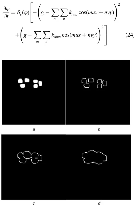
Fig. 1 Image containing a cluster of objects and its segmented images with different values forn

a Original image containing a cluster of objects

b Segmented image using piecewise constant approximation without contour length minimisation

c Segmented image using piecewise constant approximation with contour length minimisationn¼50

d Segmented image using piecewise constant approximation with contour length minimisationn¼70

Fig. 2 Synthetic star image and its segmented images with differ-ent values forn

a Original star image

b Segmented image using piecewise constant approximation without contour length minimisation

c Segmented image using piecewise constant approximation with contour length minimisationn¼300

In the next section, the results achieved by the above algorithms are presented.

3 Results

In this section, the algorithms outlined in the previous sec-tions are applied to different synthetic and real world images. In Figs. 1 and 2, we specifically address the impact of removing the contour length minimisation term in the M – S functional. Equations (6) – (8) (piecewise con-stant approximation with contour length minimisation term) are applied to the image shown in Fig. 1a with

n¼50 and n¼70. The detected contours are shown in

Figs. 1cand1d. Equations (6), (7) and (15) (piecewise con-stant approximation without contour length minimisation term) are also applied to the image ofFig. 1a. The segmen-ted image is depicsegmen-ted inFig. 1b. It is clear fromFig. 1that when the contour length minimisation term is included in the M – S functional, the contours detected do not corre-spond with the edges of the object in a given image. This is expected in the M – S functional, as the contour minimis-ation term smoothes the detected contour. The extent of the difference between the contours and the objects’ actual edges in a given image depends on the value chosen forn

and the image contents, i.e.kiandkoin equation (8).

Fig. 2shows another example that demonstrates the fact that in the M – S functional, the detected contours do not always correspond with objects’ edges. Equations (6) – (8) (piecewise constant approximation with contour length minimisation term) with n¼300 andn¼500 are applied Fig. 3 Noise sensitivity of the proposed algorithm

a Original noiseless image

b Image contaminated with Gaussian noise with SNR¼1.088

c Segmentation results for SNR¼1.088

d Smoothed image withm¼100 for SNR¼1.088

e Image contaminated with Gaussian noise with SNR¼0.372

f Segmentation results for SNR¼0.372

g Smoothed image withm¼100 for SNR¼0.372

h Image contaminated with Gaussian noise with SNR¼0.051

i Segmentation results for SNR¼0.051

j Smoothed image withm¼100 for SNR¼0.051

Fig. 4 Approximation of the functional using Legendre series

a Original noiseless image with a patch characterised by smooth vari-ation in brightness

b Noisy image with Gaussian noise (SNR¼1.026)

c Segmentation result using proposed algorithm based on Legendre series with the first six Legendre components

d Reconstructed image using the coefficients of the first six Legendre components

Fig. 5 Noiseless synthetic image

a Original noiseless image with two different textures

b Noisy image with Gaussian noise (SNR¼7.347)

c Segmented image using our Fourier-based algorithm using 45 Fourier components

toFig. 2aand the detected contours are depicted inFigs. 2c and2d.Fig. 2balso shows the detected contour without the contour length minimisation term using piecewise constant approximation. For illustration and comparison purposes, the detected contours are superimposed on the original image in this figure. Figs. 1 and 2 therefore demonstrate that the M – S functional without the contour minimisation term reduces to an edge detection scheme.

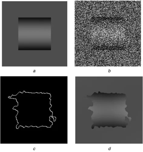
Noise sensitivity of the proposed algorithm is investi-gated inFig. 3.

A noiseless image is considered inFig. 3a, and Gaussian noise is added (SNR¼1.088) to obtain the image of

Fig. 3b. The segmented image is shown in Fig. 3cwith a Gaussian filter bandwidth of p/3, and the smoothed image depicted in Fig. 3d is obtained with m¼100. Similar results are shown in Fig. 3 for the same image with SNR¼0.372 and 0.051 with bandwidths being p/4 and

p/5 for the Gaussian filter, respectively. As observed from

Figs. 3h–j, the algorithm operates at SNR as low as 0.051. Approximation of the desired function f(x,y) using Legendre series is demonstrated inFig. 4a, which shows a patch characterised by a smooth variation in brightness against a background with a mean grey scale equal to that of the patch. This image is further contaminated with Gaussian noise (SNR¼1.026) to obtainFig. 4b. Coupled equations (20) and (21) are applied to the image of

Fig. 4bto achieve the segmented image shown in Fig. 4c using the first six components in the Legendre series. The bandwidth of the Gaussian filter was chosen as p/6. It should be noted that the both the piecewise constant (equations (6) – (8)) and continuous (equations (10) – (12)) solutions presented in [4, 19, 21] fail to segment the patch. In the case of the piecewise constant solution, this is because the mean grey level of the central object in

Fig. 4 is equal to the mean grey level of the rest of the image. Hence, there is no force to drive the evolving contour in (8). However, for piecewise continuous approxi-mation, if the initial contour is not close enough to the object to be segmented, the C – V method falls into local minima [19]. The reconstructed image formed by using the calculated coefficients of Legendre series at the conver-gence of the algorithm is depicted inFig. 4d.

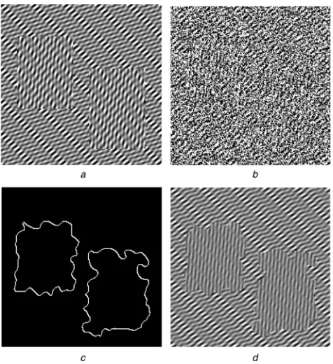
A noiseless synthetic image with two different textures is depicted in Fig. 5a. This image is contaminated with Gaussian noise (SNR¼7.347) and shown inFig. 5b. The

segmentation result using the algorithm expressed in (23) and (24) is shown in Fig. 5c. The reconstructed image using the calculated coefficients of the Fourier series is depicted inFig. 5d.

Fig. 6depicts a few iterations of the contour evolutions of the proposed Fourier-based method in this paper, with two different initial contours applied to a synthetic image with two rectangular patches with the same texture against a different background texture.

The same image shown in Fig. 6is also used inFig. 7. Zero-mean Gaussian noise is added (SNR¼1.061) to the Fig. 6 Contour evolutions of the proposed Fourier-series-based method with two different initial contours (conditions)

Fig. 7 Synthetic noisy textured image and its segmentation and reconstruction results

a Original noiseless image with two separate regions with same texture against a background texture different from those regions

b Noisy image with additive zero-mean Gaussian noise (SNR¼1.061)

c Segmented image using proposed Fourier-based algorithm using 55 Fourier components

noiseless image ofFig. 7ato obtain the noisy image shown in Fig. 7b. The algorithm described by (23) and (24) is applied to the noisy image, and the result is shown in

Fig. 7c.Fig. 7dshows the reconstructed image using the coefficients of the Fourier series. Careful inspection of the noisy image inFig. 7bdemonstrates the challenge presented to human perception to recognise the presence of the objects in the image.

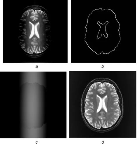
An important feature of the segmentation algorithm based on the Legendre series is the removal of distortion, which is demonstrated in Fig. 8. A magnetic resonance image dis-torted in the process of formation and digitisation is con-sidered, as shown inFig. 8a. The proposed algorithm based on the Legendre series is applied to the image, and the seg-mentation result is depicted in Fig. 8b. The distorting com-ponent in the image is estimated using the coefficients of the Legendre series calculated in the process of segmentation

and is shown inFig. 8c.Fig. 8dshows the corrected image after distortion removal from the original image.

Finally, the Fourier-based algorithm proposed in this paper is applied to an image with two different wall pat-terns, as shown in Fig. 9a. The segmentation result using 55 Fourier components is depicted inFig. 9b.

4 Conclusion

An image segmentation and smoothing method based on the M – S functional has been investigated in this paper. In this method, there is no requirement for contour length minimis-ation. Therefore the detected contours correspond to edges (discontinuities) in a given image. A two-dimensional low-pass filter is also added to improve the performance of the algorithm in a noisy environment. New methods based on Legendre and Fourier’s series are proposed to find the global minimum where the piecewise constant and continuous solutions of the problem fall in a local minimum and hence fail to perform the segmentation. Therefore this leads to an unsupervised texture segmenta-tion algorithm based on a Fourier series scheme.

5 Acknowledgment

The authors would like to thank the anonymous reviewers for their interesting and constructive suggestions, which helped to improve the presentation of this paper.

6 References

1 Kass, M., Witkin, A., and Terzopoulos, D.: ‘Snakes: active contour models’,Int. J. Comput. Vis., 1987,1, pp. 321 – 331

2 Mumford, D., and Shah, J.: ‘Optimal approximations by piecewise smooth functions and associated variational problems’, Commun. Pure Appl. Math., 1989,42, (4), pp. 577 – 688

3 Tsai, A., Yezzi, A., and Willsky, A.S.: ‘Curve evolution implementation of the Mumford– Shah functional for image segmentation, denoising, interpolation and magnification’, IEEE Trans. Image Process., 2001,10, (8), pp. 1169– 1186

4 Chan, T.F., and Vese, L.A.: ‘Active contours without edges’,IEEE Trans. Image Process., 2001,10, (2), pp. 266 – 277

5 Hintermuller, M., and Ring, W.: ‘An inexact-CG-type active contour approach for the minimization of the Mumford– Shah Functional’,

J. Math. Imaging Vis., 2004,20, pp. 19 – 42,

6 Dervieux, A., and Thomasset, F.: ‘A finite element method for the simulation of Rayleigh – Taylor instability’, in ‘Approximation methods for Navier – Stokes problems, lecture notes in mathematics’ (Springer, 1979), vol. 771, pp. 145 – 158

7 Dervieux, A., and Thomasset, F.: ‘Multifluid incompressible flows by a finite element method’,Lect. Notes Phys., 1981,11, pp. 158 – 163 8 Osher, S., and Sethian, J.: ‘Fronts propagating with

curvature-dependent speed: algorithms based on Hamilton– Jacobi formulations’,J. Comput. Phys., 1988,79, pp. 12 – 49

9 Sethian, J.A.: ‘Levet set methods: evolving interfaces in geometry, fluid mechanics, computer vision and material science’ (Cambridge University Press, 1996)

10 Caselles, V., Kimmel, R., and Sapiro, G.: ‘Geodesic active contours’. Proc. 5th Int. Conf. on Computer Vision, IEEE Computer Society Press, 1995, pp. 694 – 699

11 Caselles, V., Kimmel, R., and Saprio, G.: ‘Geodesic active contours’,

Int. J. Comput. Vis., 1997,22, (1), pp. 61 – 79

12 Sapiro, G.: ‘Geometric partial differential equations and image analysis’ (Cambridge University Press, 2001)

13 Kichenassamy, S., Kumar, A., Olver, P., Tannenbaum, A., and Yezzi, A.: ‘Gradient flows and geometric active contour models’. Fifth Int. Conf. on Computer Vision (ICCV’95), 1995, pp. 810 – 815

14 Yezzi, A., Kichenassamy, S., Kumar, A., Olver, P., and Tannenbaum, A.: ‘A geometric snake model for segmentation of medical imagery’,

IEEE Trans. Med. Imaging, 1997,16, (12), pp. 199 – 209

15 Kichenassamy, S., Kumar, A., Olver, P., Tannenbaum, A., and Yezzi, A.: ‘Conformal curvature flows: from phase transitions to active vision’,Arch. Ration. Mech. and Anal., 1996,134, (3), pp. 275 – 301 16 Aubert, G., and Kornprobst, P.: ‘Mathematical problems in image processing: partial differential equations and calculus of variations’ (Springer-Verlag, New York, 2002)

Fig. 8 Removal of distortion

a Disorted MRI image

b Segmentation using the algorithm based on the proposed Legendre series using the first six Legendre components

c Distorting image estimated using the coefficients of Legendre series calculated in the process of segmentation

d Corrected image after removing the distorting image

Fig. 9 Image with different wall patterns and segmentation result

a Image with two different wall patterns

17 Morel, J.L., and Solimini, S.: ‘Variational methods in image segmentation’ (Birkhauser, Boston, 1995)

18 Mumford, D., and Shah, J.: ‘Boundary detection by minimizing functionals’. Proc. Int. Conf. on Computer Vision and Pattern Recognition, 1985, pp. 22 – 26

19 Vese, L.A., and Chan, T.F.: ‘A multiphase level set framework for image segmentation using the Mumford and Shah model’,

Int. J. Comput. Vis., 2002,50, (3), pp. 271 – 293

20 Chan, T.F., Sandberg, B.Y., and Vese, L.A.: ‘Active contours without edges for vector-valued images’,J. Vis. Commun. Image Represent., 2000,11, pp. 130 – 141

21 Chan, T.F., and Vese, L.A.: ‘Levels et algorithm for minimising the Mumford-Shah functional in image processing’. Proc. IEEE Workshop on Variational and Level Set Methods in Computer Vision, 2001, pp. 161 – 168

22 Vese, L.A.: ‘Multiphase object detection and image segmentation’, Osher, S., and Paragios, N. (Eds.): ‘Geometrical level set methods in imaging, vision, and graphics’ (Springer Verlag, 2003), pp. 175 – 194

23 Gelfand, I.M., and Fomin, S.V.: ‘Calculus of variations’ (Prentice-Hall Inc., New Jersey, 1963)

24 Mahmoodi, S., and Sharif, B.S.: ‘Signal segmentation and denoising algorithm based on energy optimization’,Signal Process., 2005,85, (9), pp. 1845– 1851

25 Mahmoodi, S., and Sharif, B.S.: ‘Noise reduction, smoothing and time interval segmentation of noisy signals using an energy optimisation method’, IEE Proc., Vis. Image Signal Process., 2006, 153, (2), pp. 101 – 108