A Trust Model for the Analytic Hierarchy Process
Vishv Malhotra School Of Computing
GPO Box 252-100, University of Tasmania, Hobart, Tasmania 7001 AUSTRALIA
Abstract
Analytic hierarchy process (AHP) is a frequently used method for ranking alternatives. The alternatives to be ranked are modeled based on a set of criteria. The ranking computed by AHP is trusted on faith notwithstanding the fact that a model is an approximation and liable to failure. We present a model to estimate the trust in the AHP ranking. The model helps in determining if it is prudent to accept the AHP generated rankings or not.
Keywords: Analytic hierarchy process, AHP, Risk management, Decision making (processes), Multiple criteria decision.
1. Introduction
A decision exercise evaluates and ranks alternatives with respect to an objective. Save for the trivial cases, the decisions are based on the aggregated effects of a number of criteria. Quantitative decision methods compute scores for the alternatives to rank them. A score either reflects the level of benefit that the alternative delivers or it determines the cost of the alternative. Analytic Hierarchy Process (AHP) (Saaty, 1982) is a popular and pragmatic quantitative decision method. It provides a practical method to transform comparative descriptions of the problem elements into weights for the selection criteria and scores for the alternatives.
Since its inception around 1980, the AHP technique has been studied extensively (Saaty and Katz, 1994). It has been applied to a host of novel situations involving management and technical decision making. The applications range from simple selection of a product (Lai, Trueblood and Wong, 1999) to interesting applications requiring prioritisation of the software requirements based on their cost-value tradeoffs (Karlsson and Ryan, 1997). In a one-off decision situation, the AHP rankings are accepted on trust. Most papers describing the application of the technique describe a one-off decision process (Huizingh and Vrolijk, 1997). Their focus is usually on the validity of the problem model used to compute scores (Lai, Trueblood and Wong, 1999; Karapetrovic and Rosenbloom, 1999; Karlsson and Ryan, 1997).
In this paper, we focus on the relationship between the scores determined by an AHP computation and level of the trust that the ranking commands. Given the imprecision and variations in the semantics of the comparative descriptors used to describe the problem domain there is little trust in the ranking of the alternatives with near equal scores. Well-separated scores improve trust in the ranking. The goal of this paper is to assign quantitative measures on the AHP scores to express trustworthiness of the rankings.
alternative is the weighted-sum of the per-criterion scores for the alternative. The selection criteria are usually organized in a hierarchy to improve the structure and organization of the decision process. There may be a number of reasons for the scores of the alternatives to not reflect the true ranking of the alternative.
• The selection criteria may be dependent on one another or they may overlap causing certain characteristics to be implicitly included in the scores more than once.
• The set of selection criteria may fail to cover all aspects influencing the choice. This problem is the reverse of the one described in the previous dot point.
• The interactive effects between the criteria may affect the ranking of the alternatives. The technique assumes linear, additive benefits but most effects have interactive components leading to a non-linear behaviour.
What touchstone is there to say that the AHP scores reflect the true ranking of the alternatives? In this paper, we develop a trust model with three input parameters. These parameters characterize the decision environment of the AHP computation using suitable ordinal scales [Fenton and Pfleeger, 1996]. It returns a threshold value on the ratios of the AHP computed scores for the alternatives. The rankings with score ratios above the threshold value can be trusted as the benefits from accepting it out-weigh the risks.
The rest of the paper is structured in the following fashion. In Section 2, we give an overview of the trust model and introduce ordinal scales to express the input parameters to the trust model. We also include in this section, some statistical data to provide examples of, and the rationale for, the trust model and its components. Section 3 identifies the basic characteristics of the statistical data to set up mathematical formulas relating the parameters and variables of the trust model. We define the optimality condition and derive mathematical expressions to compute the optimal threshold for the specified levels of inputs to the trust model. A reader disinterested in the mathematical details may skip (all) subsections of Section 3. In Section 4, we solve these expressions and tabulate the optimal threshold values for various major values of the input parameters. The paper is concluded in Section 5 with some remarks describing the applications of the model.
2.
Overview of the Model
In this section, we give an overview of a trust model for the AHP rankings. The main components of the model are identified and we explain the part played by each component. The details of the components in the model, however, will be introduced in a later section. In this section, we also introduce some data from a decision exercise. These data will be used to provide examples and justification for the model.
2.1
A Trust Model for AHP
Analytic hierarchy process has the following basic steps:
1. The decision-maker identifies the selection criteria for the decision and organizes them into a suitable hierarchy. The comparative intensities of the criteria are determined and the weights for the criteria computed.
2. The alternatives to be ranked are identified. The alternatives are compared against each other on each criterion and a per-criterion score for the alternatives is computed.
3. The per-criterion scores of the alternatives are combined to compute overall score for each alternative. The alternatives are ranked based on their scores.
the ranking of the alternatives to be trusted. A ranking decision is trusted if the cost liability of rejecting it exceeds those of accepting it.
2.1.1 Pre-selection of the Alternatives
Alternatives under evaluation and ranking invariably pass through an implicit or even explicit pre-selection. A pre-selection step eliminates the spurious and clearly unsuited alternatives to conserve resources and simplify the decision process. A consequence of this process is to narrow the range of the scores for the alternatives.
If two alternatives have nearly equal scores, the certainty with which we would declare one better than the other depends on our expectation of the range of the scores. If the expectation is for a wide range, we reject a small difference in the scores and treat the alternatives as equals. On the other hand, if it is known that the scores will be closely placed, we readily select the alternative with the higher score as the better alternative. The pre-selection parameter aims to convey information about the expected spread of the scores into the trust model.
We shall see later that the AHP scores are best viewed as ratios. The minimum value attained by this ratio is 1. The spread of the ratios can be expressed by specifying the 90-percentile value — 90% of all likely ratios are below this value. Table 1 provides a comparative descriptive scale to specify the level of pre-selection to help a decision-maker use a textual description to express the pre-selection level.
2.1.2 The Quality of the Problem Domain Model
A model approximates the real world behaviour of the problem domain. The problem domain model used in an AHP computation comprises of a selection criteria hierarchy, intensity comparisons of the selection criteria and of the alternatives on each criterion. The AHP uses the model to compute the scores for the alternatives. The scores represent the benefits. However, the scores are approximations and some of the scores may not represent the true levels of the benefits. We have already listed reasons for this discrepancy. Consequently, the alternatives may be ranked incorrectly. The quality of a model is a measure of the decision-maker's confidence in the model. A detailed model that has been subjected to a careful validation and verification will have higher quality. A high quality model would lead to a larger fraction of the rankings computed by the AHP computation being correct.
The quality of the model is specified by indicating the percentage of the AHP computed rankings of the alternatives expected to be correct. Table 2 defines a descriptive scale to express the quality of the model parameter. The problem domain models that return less than 67% correct decisions (2 decisions in 3) are of little practical value. It is unlikely that a decision-maker would use such an inferior model in a decision exercise. These models are excluded from the measurement scale given in Table 2.
2.1.3 Risk
Comparisons
There is no cost when two alternatives are correctly ranked. However, the alternatives that are ranked incorrectly have a cost associated with the incorrect ranking. The cost represents the penalty of selecting a lower ranked alternative over a better alternative.
There is one more cost item of interest to us. This cost is incurred if we reject a ranking. The ranking of the alternatives with scores not satisfying the threshold constraint is rejected. The associated cost represents the efforts needed to rank the alternatives by other means or it may represent a loss that results if the alternatives are ranked as equals.
For the purpose of the trust model, the ratio of the cost of an incorrect decision compared to the cost of a rejected decision provides the risk comparison. Table 3 defines a scale for expressing the risk comparisons of the incorrect and rejected decisions.
2.2
Statistical Data to Validate the Trust Model
a single decision exercise. In this subsection, the decision problem is described and the data returned by these repetitions presented.
2.2.1 The Data Collection Process
The data presented was obtained from the student assignments for a second year unit. The students were introduced to the AHP technique as a multi-criteria decision-making algorithm. The topic was covered as a part of the lessons on Software Metrics.
We acknowledge the unreliability of the data collected from a student assignment. However, the data only plays a role in conceptualizing the trust model. Once the model is understood, it plays little further role in setting the coefficients in the mathematical expressions used in the trust model.
An assignment was set where the students interview clients to setup AHP tables for ranking residential properties on sale in the local real-estate market. Each student used the AHP technique to rank houses on behalf of their client. The client in turn ranked the same houses based on their preferred decision making process (checklist, intuition, or whatever). If a client reverses an AHP ranking of a pair of houses, it is noted as an incorrect AHP ranking.
The students were given a list of 12 criteria that are likely to influence a typical resident of Hobart. The set of criteria is derived from the commonly highlighted description of the houses in the local real-estate guides and newspaper advertisements. This ensures that the decision criteria are significant and cover aspects that are relevant in the local real-estate environment. One criterion in the list is special characteristics and is included to cover any special issue that the client may feel relevant and significant for their purpose.
The students were required to select four houses on sale in the local real-estate market based on the cut-off criteria that they agree with their clients. This step ensures that the students do not explore the alternatives that are obviously unacceptable to the clients.
From this class of about 90 students, some 75 students completed the assignment. Only 45 submissions were in a form that allowed us to collect the rankings of the four houses made by the AHP computation and by the client using a subjective process. Each ranking of the four houses can be viewed as a set of six decisions (pairwise rankings). That is, ranking A>B>C>D indicates the following six decisions: A>B, A>C, A>D, B>C, B>D, and C>D. The decisions made using the AHP scores may be compared against the subjective ranking provided by the clients.
Table 4 shows the subjective rankings of the houses and their corresponding AHP scores. A row lists four AHP scores. The order of the scores in a row is determined by the subjective ranking of the corresponding house by the client. For example, a row of [0.3, 0.4, 0.2, 0.1] would indicate that the top ranked house had a score of 0.3, the next one had a score of 0.4, and so on. In this row, only on one of the six decisions is the AHP ranking disagreeing with the subjective ranking made by the client. The house with a score of 0.3 is preferred by the client over the house with a score of 0.4.
2.3
An Example
To conclude the section, in this example, we assign values to the trust parameters for the assignment problem. These values will be used in the later sections to continue this example.
The pre-selection stage was based on the use of cut-off criteria to eliminate weak alternatives. Further, the indicative price of the house on sale reflects its marketability rather accurately. These two observations combine to give pre-selection level for this decision exercise of losers identified and eliminated.
The AHP model for the problem domain, however, is rated as being inconsistent. There are a number of reasons for this choice; including the casual attitude of the students and their clients towards a let-us-pretend purchase.
to the houses being ranked equal. Thus, we use the cost liability from an incorrect decision at about two (2) times the liability from a no decision.
3.
Characteristics of the AHP Scores and the Trust Model
In this section we identify the main characteristics of the decision exercise and express them as mathematical formulas. We state the condition for the optimal value for the threshold and derive a mathematical expression to compute its values for various inputs to the trust model. We will, at an appropriate point in the section, suggest to readers disinterested in the mathematical details to skip the remained of this section if they so prefer.
The analytic hierarchy process compares the selection criteria on a ratio scale. The alternatives to be ranked are compared as ratios. In turn, the scores computed for the alternatives compare them on a ratio scale. It, therefore, is meaningful to view and analyze the ratios of the scores rather than the scores per-se. The scores when expressed as ratios are more meaningful and have characteristics that do not change with the number of alternatives being compared.
To express the data in Table 4 as ratios we reorganize the rows in the table as 6 decisions. A decision compares two alternatives. We determined the ratio of the AHP scores — the higher score to the lower score — for each decision. In the rest of this paper, we refer to this ratio as a decision ratio or simply as a ratio. In the following paragraph, we introduce a few definitions. These definitions will be useful in the formalization of the mathematical relationships in the trust model.
A decision compares and ranks two alternatives. The decision is an agreement if the AHP scores and the subjective ranking of the alternatives rank them in the same order. The decision is a disagreement if the two rankings contradict each other. We introduce a threshold on the ratios of the AHP scores. The idea is to declare the decisions with ratios below the threshold value as rejected decisions. The decisions with ratios above the threshold are declared agreements or disagreements as defined earlier. A set of decisions has two obvious disjoint subsets; a set of agreements and a set of disagreements. A practicing decision-maker, uninterested in mathematical derivations, may wish to skip the mathematical details in the rest of this section and go directly to Section 4.
3.1
Distribution of the Ratios
A decision ratio can have a value equal to or greater than 1. More decisions are expected to have ratios near 1. The population density of the decisions decreases exponentially as the ratio value increases. Figure 2 plots the cumulative frequency distribution of the ratios for the decisions, agreements and disagreements for data in Table 4. In all three cases, the cumulative distribution follows the expected exponential trend. The trend curve for the cumulative distribution of the decision ratios has the form . The trend curve for the cumulative distribution of the agreements is
1
. For disagreements, it is1
.) 1 ( 4 . 2
1
−
e
− Ratio−−
e
−2.1(Ratio−1)) 1 (
4 −
−
−
e
RatioThe trend curves are approximations. The actual number of the decisions for each ratio is the sum of the number of agreements and disagreements. Thus, the true trend curve for the distribution of the
decisions is , where is the proportion of the agreements
among the decisions. This curve is also shown in Figure 2. Two trend curves for the decisions virtually coincide and are almost indistinguishable in the figure.
)
1
)(
1
(
)
1
(
−
e
−2.1(Ratio−1)+
−
q
−
e
−4(Ratio−1)q
q
∑
≤ ≤ + + = n j j i i number random Bias number random Bias e alternativ for Score 1 ) ( .The different values for the parameter
Bias
simulate different levels of the pre-selection. The study validates the following views:1. The decision ratios (for decisions, agreements and disagreements) have cumulative distribution defined by the equation
1
. The equation is parameterized by the cumulative distribution parameter δ.) 1 ( − −
−
e
δ Ratio2. The value of parameter δ is determined by the level of pre-selection performed on the alternatives being ranked.
3. The parameter δ is unaffected by the number of alternatives being ranked.
With the general nature of the distribution established, next we determine the relationship between the cumulative distribution parameters for the agreements and disagreements. These two parameters will play an important role in the formalization of the trust model. We choose to use special symbols for these parameters: ρ for the cumulative distribution parameter of the agreements and ω for the cumulative distribution parameter of the disagreements.
3.2
Proportion of Agreements and Disagreements
The quality specification of the AHP model provides the decision-makers estimate of the proportion of the agreements and disagreements among the decisions. The distribution of the decision ratios in the two disjoint sets are, however, not identical. Our goal in this sub-section is to establish suitable boundary conditions and to establish a relationship between the two cumulative distribution parameters ρ and ω.
We know that the population density of the agreements and disagreements decays exponentially as the decision ratio value is increased. For a decision ratio value of 1, the computed AHP scores for the two alternatives in the pair are equal and one would expect the decision-makers to agree (or disagree) with the ranking computed by AHP about half the time. Figure 3 plots the proportions of agreements and disagreements among all decisions as functions of the decision ratio. For each value of the ratio, r, all decisions with ratios less than or equal to r are used in the computation of the proportions. As the ratio r approaches 1, the two curves converge towards the 50% level as expected. The two curves, however, do not approach the 50% level smoothly due to the vagaries of the division with a small value in the denominator. The curves show erratic behaviour in the region near 1. Nevertheless, it is clear that the trends reach this value.
We use the observation to set the following relations:
1 → Ratio Limit 5 . 0 ) 1 )( 1 ( ) 1 ( ) 1 (
}
{
( 1) ( 1)) 1 ( = − − + − − − − − − − − Ratio Ratio Ratio e q e q e q ω ρ ρ 1 → Ratio Limit 5 . 0 ) 1 )( 1 ( ) 1 ( ) 1 )( 1 (
}
{
( 1) ( 1)) 1 ( = − − + − − − − − − − − − Ratio Ratio Ratio e q e q e q ω ρ ω
The two equations can be simplified using L’Hopital's rule to derive the following relation:
ρ
ω
)
1
(
q
q
−
=
.3.3
Cumulative Distributions of Agreements and Disagreements
90-percentile point on the cumulative distribution of the decision ratios. In what follows, we denote the 90-percentile ratio by symbol σ. Thus, when
Ratio
0
)
) 1
=
−
is set to the 90-percentile value, σ, we have
q
(
1
−
e
−ρ(σ−1))
+
(
1
−
q
)(
1
−
e
−ω(σ.
9
.The equation can be solved for ρ and ω at the various values of the AHP model quality q and pre-selection level σ. Table 5 depicts the values for ρ and ω at some of these levels of pre-selection and the quality of the AHP model.
3.4
The Optimal Threshold Ratio
A threshold value is optimal if it minimizes the total cost from the incorrect decisions and the rejected agreements. An incorrect decision is made when a disagreement appears above the threshold value. A correct decision is rejected when an agreement has the ratio below the threshold value. Risk comparison (α), see Table 3, gives the decision-makers estimate of the relative costs of the incorrect and rejected decisions.
At the optimal threshold value, τ, the number of agreements in the narrow interval [τ,τ+∆) equals α times the number of disagreements in the same interval. This leads to the following equation:
)
1
)(
1
(
)
1
)(
1
(
)}
1
(
)
1
(
{
−
−ρ(τ+∆−1)−
−
−ρ(τ−1)=
−
−
−ω(τ+∆−1)−
−
−
−ω(τ−1)α
q
e
q
e
q
e
q
e
The equation has the solution
1
1
log
(
α
)
ρ
ω
τ
e−
+
=
.4.
The Optimal Threshold Values and Other Results
We have now established all mathematical relations needed to evaluate the trust thresholds for various input values to the trust model. In this section, we tabulate the optimal threshold values. We also tabulate the expected performances of the decision exercise if these thresholds are used.
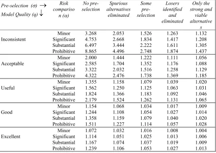
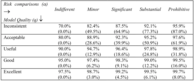
In Table 6 we compile the optimal threshold (τ) values at the major points on the input parameter scales of the trust model. The optimal threshold value is determined by three parameters – pre-selection (σ), model quality (q), and risk comparisons (α). The first two parameters are represented as the major columns and major rows respectively in the table. The last parameter determines the minor row for the threshold value. These minor rows are listed, once for each major row, under the column titled Risk comparison (α). Thus, suppose we wish to determine the optimal threshold value at the following values of the inputs: σ = losers identified and eliminated; q = inconsistent; and α = minor. We read the threshold value in Table 6 under the column titled Losers identified and eliminated, in row titled Inconsistent and against the minor row titled Minor. The optimal threshold value is 1.263. Table 7 provides the performance levels of the decision process when it has been augmented with the trust model and the decisions with ratios less than the threshold are rejected. Interestingly, the pre-selection plays no role in determining the performance levels of the AHP computation. We use two indicators for the performance. First performance indicator is the proportion of the agreements in the decisions satisfying the threshold constraint. As the threshold value rises, this performance indicator improves. However, the improvement comes at a price. As the threshold value rises, a smaller fraction of the all decisions satisfies the threshold constraint. The fraction of decisions rejected is the other performance indicator shown in Table 7.
4.1
The Example Continued
Further, Table 7 indicates that for the specified values of the input parameters, the model predicts that about 49.5% of the decisions will be rejected, as they do not meet the threshold requirement. However, of the decisions satisfying the threshold constraint 82.4% decisions are expected to be agreements (correct). It is worthwhile to note that the underlying problem domain model is rated as inconsistent and we expect only 70% correct decisions from an inconsistent model.
The actual check on the data in Table 4 based on the threshold of 1.263 indicates that 120 decisions out of 270 have a decision ratio below the threshold. There are 150 decisions satisfying the threshold requirement, of these 126 are agreements. This gives a rejection rate (decisions not made) of 44.5% with 84% of the decisions made being correct. This is slightly better performance than the one predicted. The better than expected performance is attributable to the problem domain model used in the AHP computation which returns about 73% correct decisions; a little, more than the 70% benchmark used for an inconsistent model in Table 2.
5. Conclusions
The main goal of the proposed model is to establish a mechanism for determining if it is prudent to accept the AHP computed ranking of the alternatives or not. The model is simple and requires three easy-to-describe estimates as inputs. The AHP computation process remains unaltered. Once the scores have been computed, the threshold constraint can be applied to determine if some rankings are untrustworthy. The rankings that are determined to be untrustworthy should be carefully reviewed and appropriate decisions made to avoid risks from the incorrect rankings.
The trust analysis benefits the decision process in other ways too. One application of the trust model is to increase the accuracy of the AHP ranking. We showed in an example that even an inconsistent problem domain model can be combined with a suitable trust analysis to return decisions with better consistency.
As another application, the trust model provides an indication of the area where efforts may be concentrated to improve the performance of the decision process. In the absence of a trust model, one would exclusively focus on the problem domain model to improve the ability to rank the alternatives correctly. The trust model may provide other cost-effective avenues for similar levels of gain in the ability to rank correctly.
The trust model has applications even outside the domain of AHP computation. For an interesting application in the Internet domain, consider a broker who helps the consumers find the service providers. The broker maintains information on a number of service providers. A consumer contacts the broker to select a service provider who meets their needs the best. In this scenario, the range of the variety of the service providers defines the pre-selection parameter. The matching algorithm implemented by the broker determines the quality parameter of the problem domain model. The consumer can indicate their keenness to receive service or opt out if a close match is not available by specifying the risk comparison parameter of the model. Thus, the broker can help consumers with different levels of demand and attitude towards obtaining service from the alternate sources. In this domain, the trust model is providing some of the guarantees that are usually ensured through a post-selection manual validation of the rankings.
6. Acknowledgements
The author would like to thank his colleagues Nicole Clark and Julian Dermoudy for their help in improving the clarity of the paper and its presentation. A preliminary version of the results in the paper were presented at MS2000 conference (Malhotra, 2000).
7. References
Huizingh, E.K.R.E. and H.C.J. Vrolijk 1997. Extending the Applicability of the Analytic Hierarchy Process, Socio-Economic Planning Science, Vol. 3, No 1, 29-39.
Karapetrovic, S. AND E.S. Rosenbloom. 1999. A Quality Control Approach to Consistency Paradox in AHP, European Journal of Operation Research, Vol. 119, 704-718.
Karlsson, J AND K. Ryan. 1997. A Cost-Value Approach for Prioritizing Requirements, IEEE Software, Vol. 14(5),. 67-64. Lai, V.S., R.P. Trueblood AND B.K. Wong. 1999. Software Selection: a case study of the application of the analytical
hierarchical process to the selection of a multimedia authoring system, Information & Management, Vol. 36, 221-232. Malhotra, V. 2000. Modelling Risks from Errors in Decision Algorithms, In: Hamza, M.H. (editor) Proc. of IASTED
International Conf. Modelling and Simulation (MS2000), Pittsburgh May 2000, IASTED/ACTA Press, Anaheim, 168-174.
Saaty, T.L. 1982. Decision Making for Leaders, Lifetime Learning Publications, Belmont, Ca.
Saaty, T.L. AND J.M. Katz. 1994. Highlights and Critical Points in the Theory and Application of the Analytic Hierarchy Process, European Journal Operation Research, Vol. 74(3), 426-447.
Table 1: Scale for describing the level of pre-selection of the alternatives prior to an AHP computation.
Descriptive term Comparative intensity
on Saaty scale
90-percentile value for the ratios (σ)
No pre-selection 1 10
Spurious alternatives eliminated 3 5
Some pre-selection 5 3
Losers identified and eliminated 7 2
Only the strong and viable alternatives 9 1.5
Table 2: Scale for a descriptive indication of the quality of the problem domain model used in an AHP computation.
Descriptive term Comparative intensity on Saaty scale
Expected fraction of total decision being correct (q)
Inconsistent 1 70%
Acceptable 3 80%
Useful 5 90%
Good 7 95%
[image:9.595.85.514.265.360.2]Excellent 9 97.5%
Table 3: Scale for comparing the cost of an incorrect decision with the cost of a rejected decision Descriptive term Comparative intensity on
Saaty scale Cost multiplier (α)
Indifferent 1 1
Minor 3 2
Significant 5 3
Substantial 7 5
Prohibitive 9 10
Table 4: AHP scores of houses ranked by their subjective appeals.
AHP Scores for house ranked
First Second Third Fourth (last)
[image:9.595.84.515.407.501.2]AHP Scores for house ranked
[image:10.595.112.485.73.634.2]0.266 0.290 0.240 0.203 0.286 0.235 0.214 0.265 0.307 0.348 0.233 0.112 0.243 0.308 0.256 0.192 0.265 0.242 0.254 0.240 0.275 0.332 0.225 0.168 0.225 0.295 0.240 0.240 0.161 0.282 0.241 0.315 0.254 0.315 0.226 0.204 0.272 0.329 0.285 0.116 0.269 0.315 0.210 0.206 0.295 0.199 0.291 0.215 0.280 0.288 0.263 0.169 0.238 0.220 0.285 0.258 0.315 0.260 0.260 0.165 0.448 0.176 0.208 0.169 0.450 0.100 0.300 0.150 0.221 0.171 0.346 0.262 0.237 0.321 0.205 0.237 0.157 0.227 0.262 0.354 0.310 0.210 0.250 0.230 0.273 0.302 0.302 0.123 0.270 0.240 0.270 0.220 0.295 0.295 0.232 0.179 0.316 0.304 0.238 0.137 0.263 0.235 0.221 0.295 0.300 0.250 0.230 0.220 0.364 0.216 0.287 0.133 0.329 0.229 0.240 0.202 0.330 0.259 0.242 0.169 0.290 0.230 0.270 0.200 0.290 0.254 0.189 0.266 0.320 0.280 0.190 0.190 0.305 0.202 0.301 0.191 0.286 0.292 0.247 0.174 0.302 0.302 0.123 0.273 0.315 0.264 0.238 0.183 0.320 0.230 0.252 0.199 0.318 0.323 0.220 0.138
Table 5: The cumulative distribution of the ratios for agreements is given by
1
and for disagreements by1
.) 1 ( − −
−
e
ρ Ratio )1 ( − −
−
e
ω RatioPre-selection (σ)
→
Model Quality (q)↓
No
pre-selection alternatives Spurious eliminated
Some
pre-selection identified Losers and eliminated
Strong and viable alternatives
ω =0.51 ω =1.15 ω =2.31 ω =4.61 ω =9.22 Acceptable ρ =0.23
ω =0.92
ρ =0.52
ω =2.08
ρ =1.04
ω =4.16
ρ =2.08
ω =8.32
ρ =4.16
ω =16.6
Useful ρ =0.24
ω =2.20
ρ =0.55
ω =4.94
ρ =1.10
ω =9.89
ρ =2.20
ω =19.8
ρ =4.39
ω =39.6
Good ρ =0.25
ω =4.75
ρ =0.56
ω =10.7
ρ =1.13
ω =21.4
ρ =2.25
ω =42.8
ρ =4.50
ω =85.6
Excellent ρ =0.25
ω =9.87
ρ =0.57
ω =22.0
ρ =1.14
ω =44.4
ρ =2.28
ω =88.8
ρ =4.55
[image:11.595.88.512.225.525.2]ω =178
Table 6: The optimal threshold (τ) values for various levels inputs to the trust model. Pre-selection (σ)
→
Model Quality (q)
↓
Risk compariso
n (α)
No pre-selection Spurious alternatives eliminated Some pre-selection Losers identified and eliminated Only the strong and viable alternative s
Inconsistent Significant Minor Substantial Prohibitive 3.268 4.753 6.497 8.865 2.053 2.668 3.444 4.496 1.526 1.834 2.222 2.748 1.263 1.417 1.611 1.874 1.132 1.208 1.305 1.437 Acceptable Minor Significant Substantial Prohibitive 2.000 2.585 3.322 4.322 1.444 1.704 2.032 2.476 1.222 1.352 1.516 1.738 1.111 1.176 1.258 1.369 1.056 1.088 1.129 1.185 Useful Significant Minor
Substantial Prohibitive 1.355 1.562 1.824 2.179 1.158 1.250 1.366 1.524 1.079 1.125 1.183 1.262 1.039 1.063 1.092 1.131 1.020 1.031 1.046 1.065 Good Minor Significant Substantial Prohibitive 1.154 1.244 1.358 1.511 1.068 1.108 1.159 1.227 1.034 1.054 1.079 1.114 1.017 1.027 1.040 1.057 1.009 1.014 1.020 1.028 Excellent Significant Minor
Table 7: Performance of an AHP computation in ranking the alternatives when combined with the trust analysis. Numbers outside the parentheses are the percentages of the decisions correct. Numbers enclosed in the
parentheses give the percentages of the decisions that are rejected. Risk comparisons (α)
→
Model Quality (q)
↓
Indifferent Minor Significant Substantial Prohibitive
Inconsistent 70.0%
(0.0%) (49.5%) 82.4% (64.9%) 87.5% (77.3%) 92.1% (87.0%) 95.9% Acceptable 80.0%
(0.0%)
88.9% (28.6%)
92.3% (39.9%)
95.2% (50.9%)
97.6% (61.9%) Useful 90.0%
(0.0%)
94.7% (12.9%)
96.4% (18.6%)
97.8% (24.8%)
98.9% (31.8%) Good 95.0%
(0.0%) (6.2%) 97.4% (9.1%) 98.3% (12.2%) 99.0% (16.0%) 99.5% Excellent 97.5%
(0.0%)
98.7% (3.0%)
99.2% (4.5%)
99.5% (6.1%)