Grid Resolution for the Simulation of Sloshing using CFD
Bernhard Godderidge
∗
, Mingyi Tan
∗
, Chris Earl
∗∗
& Stephen Turnock
∗
*Fluid-Structures Interaction Research Group, School of Engineering Sciences, University of Southampton, Highfield, Southampton SO17 1BJ, UK
**BMT SeaTech, Grove House, 7 Ocean Way, Southampton SO14 3TJ, UK
Corresponding author’s email: [email protected]
Introduction
Sloshing occurs when a tank is partially filled with a liq-uid and subjected to an external excitation force [1]. Ships with large ballast tanks and liquid bulk cargo carriers, such as very large crude carriers (VLCCs), are at risk of expo-sure to sloshing loads during their operational life [2]. The inclusion of structural members within the tanks dampens the sloshing liquid sufficiently in all but the most severe cases. However, this approach is not used for Liquefied Natural Gas (LNG) carriers and the accurate calculation of the sloshing loads is an essential element of the LNG tank design process [3, 4].
The increase in global demand for LNG has resulted in a new generation of LNG tankers with a capacity in excess of 250,000 m3, compared to 140,000 m3 today. A pre-requisite for the safe operation of these LNG tankers is an accurate calculation of the sloshing loads experienced by the containment system [5, 6].
The work of Abramson [7] summarizes the methods available in modern sloshing analysis, and Ibrahim [8] gives an up-to-date survey of analytical and computational sloshing modeling techniques. A more general modeling technique is the solution of the Navier-Stokes equations using Computational Fluid Dynamics (CFD). Some recent examples of CFD sloshing simulation include Hadzic et al. [9], Aliabadi et al. [10], Standing et al. [11], Kim et al. [12], Rhee [13] and El Moctar [14].
Sloshing flows are treated as a transient problem in CFD. While the number of sloshing oscillations can vary, a large number of time steps, usually O(102)to O(103)per oscil-lation are required. Design optimization or the use of a numerical wave tank to gather statistical sloshing pressure data [15] requires long simulation times or multiple runs. Parameters such as time step size, grid spacing and model choice directly influence the complexity and computational cost of a CFD model.
A sway-induced resonant sloshing flow in a 1.2 m x 0.6 m rectangular container is investigated using a commer-cial Navier-Stokes CFD code. The selected computational model was validated using experimental pressure data from
Hinatsu [16] by Godderidge et al. [17, 18]. The effect of grid spacing when capturing impact pressure caused by an enclosed air bubble is investigated. It is found that local flow features are best suited to indicate that the flow is suf-ficiently well resolved. These findings are further inves-tigated using larger, geometrically similar sloshing tanks. The initial grid geometry is used to simulate the scaled sloshing flow at two and four times the initial grid size. Then, the grid is refined to give the same mesh spacing as in the first problem.
Sloshing Problem
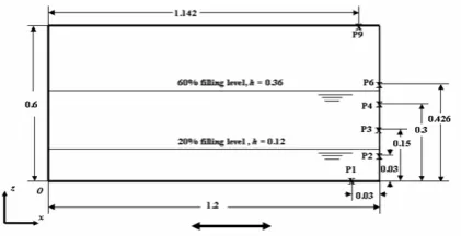
Sloshing in rectangular container, induced by pure sway motion, is investigated in the present study. Figure 1 shows the tank dimensions, locations of pressure monitor points and axis system orientation. The CFD model was vali-dated using the experimental steady state sloshing pres-sures given by Hinatsu [16]. The tank displacement is given by
x=A sin
2π
T t
, (1)
[image:1.595.316.527.642.750.2]where A is the displacement amplitude, T the sloshing pe-riod and t the elapsed time. In the current case, the tank motion is in the x-direction only, as indicated in Figure 1. The first part of the investigation is focused on a resonant sloshing flow at 20% filling level, where A=0.06 m and T=1.74 sec. Subsequently, a near-resonant sloshing flow with A=0.015 m and T=1.404 sec is considered.
Figure 1: The sloshing problem used for CFD validation (all
The fluid interaction models for the numerical simula-tion of sloshing can be implemented using the volume frac-tion of each fluid to determine the fluid mixture properties. This is a homogeneous multiphase model. It is analogous to the volume of fluid (VOF) method developed by Hirt and Nichols [19], but it includes a simplification as the free surface pressure boundary condition is neglected. A more general but computationally more expensive approach is an inhomogeneous multiphase model, where the solution of separate velocity fields for each fluid is matched at the fluid interfaces using mass and momentum transfer models [20]. An inhomogeneous viscous compressible multiphase flow with two phasesαandβis governed by the conserva-tion of mass for the compressible phaseα
∂ ∂t(rρ) +
∂ ∂xi
(rρui) =m+Γαβ, (2)
whereΓαβis mass transfer between the phases and m mass sources, ρ density, r volume fraction and ui velocity of phaseα. The conservation of momentum for phaseα is given as
∂
∂t(rρui) +
∂ ∂xj
(rρuiuj) =−r∂ p
∂xi
+
+ ∂
∂xj
rµ
∂u
i
∂xj
+∂uj
∂xi
+MΓ+Mα+bi, (3)
where biare body forces, Mαforces on the interface caused by the presence of phaseβ, µ the dynamic viscosity and the term MΓ=Γαβuβi −Γβαui
interphase momentum trans-fer caused by mass transtrans-fer. If the fluid is compressible, Equations (2) and (3) are closed using an energy equa-tion, or an equation of state if the compressible fluid can be treated as an ideal gas [21]. A discussion of the fluid interface forces is given by Godderidge et al. [22].
As a full set of conservation equations has to be solved for each phase, the computational effort required for the inhomogeneous model has been found to be 2.3 times greater1than for the homogeneous model [22]. However, Brennen [23] finds that if two conditions derived from par-ticle size parameter, mass parameter and parpar-ticle Reynolds number are violated, the inhomogeneous multiphase model (Equations 2 and 3) should be used. It is observed that for the current problem, the particle Reynolds number condi-tion is not satisfied. This suggests that the use of an inho-mogeneous multiphase model is required for the analysis of the current problem.
The computational models used in the sloshing studies are summarised in Table 1. The selection is based on the sensitivity study by Godderidge et al. [17]. It was found that the pressure histories of the current fluid model bination differed by less than 0.1% from the fully com-pressible model but required 20% less computational time. Kim et al. [12] showed that the sloshing pressure is not influenced by the inclusion of a turbulence model, but the use of a standard k−εturbulence model with a scalable 1The simulations were run on a 64 bit, 2.2 GHz processor with 2 GB
of RAM at the University of Southampton Iridis 2 computational facility
wall function aided convergence when using a viscous flow model [17]. The high resolution scheme for spatial dis-cretization varies between a first and second order upwind scheme depending on the gradient [21]. The grids used for the various studies are detailed in the sections describing the respective results.
Table 1: Computational models used for sloshing simulations
Parameter Setting
Water Incompressible fluid
Air Ideal gas
Multiphase model inhomogeneous Sloshing motion Body force
Turbulence model Standard k−εwith scalable wall function
Spatial discretization High resolution
Time discretization Second order backward Eu-ler
Timestep control Root-mean-square (RMS) Courant number=0.1 Convergence control RMS residual<10−5
The investigation of sloshing in geometrically similar containers required the calculation of an appropriate slosh-ing excitation. The nature of the excitation, given in Equa-tion (1), is maintained but the amplitude and frequency are adjusted. The sloshing period is 95% of the resonant period which depends on the tank size. The resonant freqnecy for each case is calculated from potential theory as
ω2 n= πg a tanh πh a , (4)
where a is the tank length, g gravity and h the filling level. The amplitude of the sloshing excitation is adjusted using the sloshing velocity, which may be obtained by differenti-ating Equation (1). Taking the excitation velocity as a char-acteristic velocity, the following non-dimensional scaling parameter based on the Froude number [7] can be used
˙ xl ˙ xL = √ gDl √ gDL , (5)
where Dland DLare characteristic length scales.
Impact bubble
2(a): Bubble size dependence on grid 2(b): Air bubble formation
Figure 2: Air entrainment bubble formed during sloshing impact
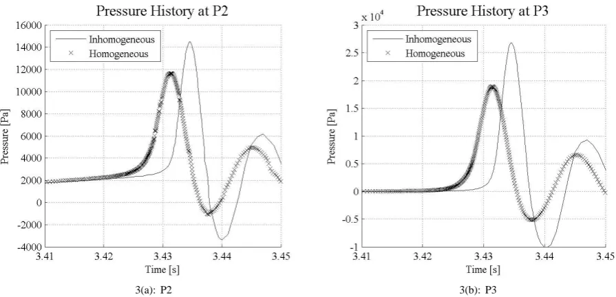
[image:3.595.69.517.307.523.2]3(a): P2 3(b): P3
Figure 3: Pressure history at P2 (left) and P3 (right)
The sloshing flow is simulated on a hybrid grid with a refined region indicated in Figure 2. Table 2 gives the grid particulars in the refined region. Figure 2(a) shows the grid dependence of the air bubble dimensions and the formation of the air bubble is illustrated in Figure 2(b).
Table 2: Grid refinement for sloshing impact
Grid Hex. horizontal (first node) vertical
(mm) (mm)
Grid a 408 0.30 12
Grid b 2552 0.10 3.5
Grid c 4602 0.05 2.0
Grid d 16284 0.02 0.5
Figure 3 shows the pressure history during fluid impact at P2 and P3 for the 20% filling level. In both cases, the ho-mogeneous multiphase model gives, for the identical fluid
model and initialisation, a significantly lower pressure than the inhomogeneous model. Figure 4 shows that the direc-tion of the water prior to impact depends on the selected multiphase model. The inhomogeneous flow predicted wa-ter velocity is inclined 14.0◦from the horizontal, while the homogeneous model estimated the velocity vector inclina-tion at 40.3◦.
Figure 4: Water flow 0.05 cm before impact
5(a): Perpendicular grid spacing
[image:4.595.314.522.73.201.2]5(b): Longitudinal grid spacing
Figure 5: Pressure dependence on local perpendicular (top) and
longitudinal (bottom) flow feature resolution
Tank Size Variation
Equation (1), which describes the sloshing excitation, can be rewritten as
x=αA sin
2π
T t
, (6)
whereα is a constant. Using Equation (4) and (5), the sloshing excitation can be adjusted for kinematic similitude corresponding to the tank size. The computed values are given in Table 3.
The grid used for Case 1 which consists of 9360 ele-ments is shown in Figure 6. Grid size and time discretisa-tion parameters were determined from Ref [25]. This grid is then resized using the appropriate size factors for cases 2 and 3. The number of grid cells remains constant but the size of each element increases accordingly. A second set of grids (grid 2 and 3) is constructed for cases 2 and 3 tively. They contain 38,319 and 153,273 elements respec-tively and they have the same cell size as the grid used for
Table 3: Systematic tank size variations
Parameter Case 1 Case 2 Case 3
Sloshing Tank
Size factor 1 2 4
Length 1.2 m 2.4 m 4.8 m
Height 0.6 m 1.2 m 2.4 m
Filling Level 60% 60% 60%
Excitation
α 1 1.961 3.922
A 0.015 m 0.015 m 0.015 m T10 1.474 sec 2.044 2.890
[image:4.595.70.283.190.477.2]case 1. The computational models used in the simulations are given in Table 1.
Figure 6: Typical hybrid grid used in CFD investigations. The
grid contains 8652 hexahedral and 708 wedge elements
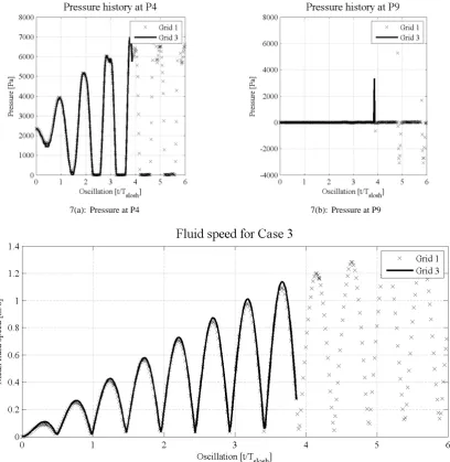
Figures 7(a) and 7(b) shows the pressure histories at monitor points P4 and P9 respectively for case 3 predicted using grids 1 and 3. At P4, which is dominated by the static pressure component, the pressure histories show rea-sonable agreement. At P9, the pressure spike captured on grid 3 is not observed using grid 1. Mean fluid speed is less susceptible to grid effects. Figures 7(c) and 7(d) show the mean fluid velocity, which is computed as
Mean fluid speed=
∑
mass mi|vi|
∑
mass mi
. (7)
Figure 7(c) shows acceptable agreement between the mean fluid speed history observed using grids 1 and 3. Finally, mean fluid speed appears to be a quantity well suited for scaling with Equation (5) as shown in Figure 7(d). While the scaled and observed speed histories are out of phase when using grid 1, the predicted magnitudes show good agreement with those observed when scaling from grid 2.
Concluding Remarks
[image:4.595.322.517.251.351.2]7(a): Pressure at P4 7(b): Pressure at P9
7(c): Grid dependence of fluid momentum
[image:5.595.94.503.75.495.2]7(d): Predicted and observed fluid momentum
grid to observe critical flow features and repeat the simula-tion on a grid that adequately resolves local flow features by including information from e.g. Ref [27].
When increasing the tank size, local impact pressures are not captured unless the grid is refined according to the flow field. Moreover, the scaling of sloshing pressures remains a task of some difficulty. The mean fluid velocity defined in Equation (7) appears to be a quantity better suited to scaling. The magnitude of the mean fluid velocity of case 3 is estimated with good accuracy based on grids 1 or 2. However, a lag develops between the solution estimated from grid 1 and the mean fluid momentum obtained from grid 3.
The scaling of mean fluid velocity requires further study for additional validation. The simulations for the system-atic variations of tank size should be extended to at least 10 oscillations. A further tank size of 9.6 m by 4.8 m should be included to confirm the scaling properties of mean fluid momentum. Ultimately, the mean fluid velocity may pro-vide an alternative design criterion more suitable for scal-ing when assessscal-ing the safety of LNG tanks.
References
[1] Harald Olsen. What is sloshing? In Seminar on Liquid
Sloshing. Det Norske Veritas, 1976.
[2] E Rizzuto and R Tedeschi. Surveys of actual sloshing loads onboard of ships at sea. In NAV 97: International Confer-ence on Ship and Marine Research, 1997.
[3] Robert L Bass, E B Bowles, and P A Cox. Liquid dynamic loads in LNG cargo tanks. SNAME Transactions, 88:103– 126, 1980.
[4] T Knaggs. New strides in ship size and technology. Gas Ships: Trends and Technology., 2:1–4, 2006.
[5] Sungkon Han, Joo-Ho Heo, and Sung-Geun Lee. Critical design issues of new type and large LNG carriers. In Pro-ceedings of the 15th International Offshore and Polar Engi-neering Conference, 2005.
[6] James Card and Hoseong Lee. Leading technology for next
generation of LNG carriers. In Proceedings of the 15th
International Offshore and Polar Engineering Conference, 2005.
[7] H Norman Abramson. The dynamic behavior of liquids in moving containers, with applications to space vehicle tech-nology. Technical Report SP-106, National Aeronautics and Space Administration, 1966.
[8] Raouf A Ibrahim. Liquid Sloshing Dynamics. Cambridge University Press, 2005.
[9] I Hadzic, Frank Mallon, and M Peric. Numerical simula-tion of sloshing. Technical report, Technische Universit¨at Hamburg-Harburg, 2002.
[10] Shahrouz Aliabadi, Andrew Johnson, and Jalal Abedi. Comparison of finite element and pendulum models for sim-ulation of sloshing. Computers and Fluids, 32:535–545, 2003.
[11] R G Standing, S Amaratunga, F Lopez-Calleja, S Orme, and R Eichaker. Marine hydrodynamics modelling using CFD. In CFD 2003: Computational Fluid Dynamics Technology in Ship Hydrodynamics, 2003.
[12] Yonghwan Kim, Jungmoo Lee, Young-Bum Lee, and Yong-Soo Kim. Sensitivity study on computational parameters for the prediction of slosh-induced impact pressures. In Pro-ceedings of the 15th International Offshore and Polar Engi-neering Conference, 2005.
[13] Shin Hyung Rhee. Unstructured grid based
Reynolds-Averaged Navier-Stokes method for liquid tank sloshing. Transactions of the American Society of Mechanical Engi-neers, 127:572–582, 2005.
[14] Ould El Moctar. Assessment for tankers. Shipping World and Shipbuilder, 204:28–31, 2006.
[15] Mateusz Graczyk, Torgeir Moan, and Olav Rognebakke. Probabilistic analysis of characteristic pressure for LNG tanks. Journal of Offshore Mechanics and Arctic Engineer-ing, 128:133–144, 2006.
[16] Munehiko Hinatsu. Experiments of two-phase flows for
the joint research. In Proceedings of SRI-TUHH
mini-Workshop on Numerical Simulation of Two-Phase Flows. National Maritime Research Institute & Technische Univer-sit¨at Hamburg-Harburg, NMRI, 2001.
[17] Bernhard Godderidge, Mingyi Tan, and Stephen Turnock. A verification and validation study of the application of com-putational fluid dynamics to the modelling of lateral slosh-ing. Ship Science Report 140, University of Southampton, 2006.
[18] Bernhard Godderidge, Mingyi Tan, Stephen Turnock, and Chris Earl. Multiphase CFD modelling of a lateral sloshing tank. In Numerical Towing Tank Symposium, 2006.
[19] C W Hirt and B D Nichols. Volume of fluid (VOF) method for the dynamics of free boundaries. Journal of Computa-tional Physics, 39:201–225, 1981.
[20] M Ishii and T Hibiki. Thermo-Fluid Dynamics of
Two-Phase Flow. Springer Verlag, 2006.
[21] Ansys Inc. CFX-10 User’s Guide, 2005.
[22] B Godderidge, S Turnock, M Tan, and C Earl. An inves-tigation of multiphase CFD modelling of a lateral sloshing tank. Computers and Fluids (submitted).
[23] C E Brennen. Fundamentals of Multiphase Flow. Cam-bridge University Press, New York, 2005.
[24] Wu-Ting Tsai and Dick K. P Yue. Computation of non-linear free surface flows. Annual Review of Fluid Mechan-ics, 28:249–278, 1996.
[25] B Godderidge, M Tan, C Earl, and S Turnock. Boundary layer resolution for modeling of a sloshing liquid. In Inter-national Society of Offshore and Polar Engineers, 2007.
[26] American Bureau of Shipping. Guidance notes on strength assessment of membrane-type LNG containment systems under sloshing loads. Technical report, American Bureau of Shipping, 2006.