Structure evolving systems and control in integrated design

      

City, University of London Institutional Repository

Citation

: Karcanias, N. (2008). Structure evolving systems and control in integrated

design. Annual Reviews in Control, 32(2), pp. 161-182. doi: 10.1016/j.arcontrol.2008.07.004

This is the accepted version of the paper.

This version of the publication may differ from the final published

version.

Permanent repository link:

http://openaccess.city.ac.uk/14045/

Link to published version

: http://dx.doi.org/10.1016/j.arcontrol.2008.07.004

Copyright and reuse:

City Research Online aims to make research

outputs of City, University of London available to a wider audience.

Copyright and Moral Rights remain with the author(s) and/or copyright

holders. URLs from City Research Online may be freely distributed and

linked to.

Structure Evolving Systems and Control in Integrated Design” ANNUAL REVIEWS IN CONTROL 18-06- 08

“Structure Evolving Systems and Control in Integrated Design”

Nicos Karcanias

Control Engineering Centre,

School of Engineering and Mathematical Sciences, City University, Northampton Square, London EC1V 0HB, UK

e.mail: [email protected]

Abstract

Existing methods in Systems and Control deal predominantly with Fixed Systems, that have been designed in the past, and for which the control design has to be performed. The new paradigm of Structure Evolving Systems (SES),

expresses a new form of system complexity where the components, interconnection topology, measurement-actuation schemes may not be fixed, the control scheme also may vary within the system-lifecycle and different views of the system of varying complexity may be required by the designer. Such systems emerge in many application domains and in the engineering context in problems such as integrated system design, integrated operations, re-engineering, lifecycle design issues, networks etc. The paper focuses on the Integrated Engineering Design (IED), which is revealed as a typical structure evolution process that is strongly linked to Control Theory and Design type problems. It is shown, that the formation of the system, which is finally used for control design evolves during the earlier design stages and that process synthesis and overall instrumentation are critical stages of this evolutionary process that shapes the final system structure and thus the potential for control design. The paper aims at revealing the control theory context of the evolutionary mechanism in overall system design by defining a number of generic clusters of system structure evolution problems and by establishing links with existing areas of control theory. Different aspects of

1.Introduction

Complex Systems emerge in many disciplines and domains and have many interpretations andimplications. Different communities view complexity from their domain specifics and frequently the dialogue between communities such as biologists, physicist, economists, sociologists, computer scientists and engineers becomes difficult, or impossible. Mathematical Systems and Control Theory have the potential to provide the unifying framework (language and concepts) and the required tools (analysis, synthesis) for studying such problems, as long as it develops to handle some of the new challenging paradigms emerging from the widening field of applications. The paper deals with the form of complexity inherent in the new paradigm of Structure Evolving Systems (SES), asthis emerges in the context of system, or integrated design. Such forms of systems emerge in many applications and are characterised by a variability of the system structure, its components and possibly its environment, in a way that defines an evolution of the system structure and the associated properties. Integrated Design (ID) (Karcanias, 1994a, 2000) is a challenging task in many application areas (aeronautics, process systems (Stephanopoulos, 1984) etc) and defines the focus of our study of the SES paradigm by providing a number of mostly open structural systems and control problems. The case of process systems (Perkins,1990), (Rijnsdorp,1991) provides the additional focus of our current study. The aim of this paper is to identify the open issues which have a clear systems and control character and establish the links with existing areas in control.

Existing methods in Systems and Control deal predominantly with “fixed systems”, that is those where the components, interconnection topology, measurement-actuation schemes, systems environment and control structures are fixed. The process of overall design of a system (process synthesis - global instrumentation - control) has a cascade nature (Karcanias, 2000) and this introduces a notion of “shaping”, evolution of the model and thus of the resulting system properties. In fact, as we go through the different design stages we have an evolution of structure, topology, properties and behaviour of the overall system. Design is an iterative process and thus it is characterised by “early” and “late” stages. “Early design” requires evaluation of many alternatives using simple models and methodology (EPIC, 1989), (Rijnsdorp, 1991) whereas “late design” uses models of greater complexity and accuracy and requires more detailed evaluation of performance. Decision making at each stage is largely based on local criteria; this is a consequence of overspecialisation and lack of a holistic co-ordination of design methodology. Similar nature problems arise in the re-engineering of existing systems/networks in their upgrading to meet new requirements and performance demands. This may involve physical addition (growth), or removal (death) of parts of the system and represents evolution of a given system shell along a number of possible paths by intervening on the subsystem components, process synthesis/topology of interconnections, and overall instrumentation. Key questions that arise relate to modelling such forms of evolution, and then express model evolution in terms of the structural features and properties of the respective models. The major challenge is managing complexity involving the control, or direction of such an evolutionary process along “paths” with desirable properties. This requires a methodology that is based on results characterising the potential for evolution of system properties (genetic selection of alternatives), explain the link of structure to invariants and performance indicators, characterise model uncertainty within a given system structure, define the “good” or “bad” potential for design, and provide means for addressing “structure assignment” problems. Responding to such tasks requires a new and richer form of Control Theory that is empowered to deal with the management of structure evolution.

The need for integrating process and control design has been recognised in the Process, Aerospace and other areas of applications, but with a few exceptions (EU Project SESDIP (1994)), little attention has been given in the development of an integrated Systems and Control Theory Based Framework that may integrate the traditional design stages, such as Process Synthesis (PS), Global Instrumentation (GS) and finally Control Design (CD). Design is a cascade and complex process that is characterised by different forms of system evolution. This evolution has three main features: The first is a natural evolution of the system structure as this is shaped through the design stages from conceptualisation, to process synthesis, global instrumentation and finally control design and it is referred to as

cascade structural evolution. The second stems from the need to address design and decision problems at “early” and “late” stages of system design (as part of an iterative design cycle) using models with a variability in their complexity and it is referred to as design time evolution. The third deals with the type of evolution linked to re-engineering of a given structure and will be referred to as structural growth-death evolution. The paper aims to describe those three forms of system evolution from a control theoretic viewpoint, review existing approaches and define a research agenda for the structural system methodologies that can deal with such issues. The proposed structural approach is based on defining and studying a number of partial problems, which when combined may provide the essentials for a control theoretic framework for systems integration. The paper addresses control theory issues linked to overall system design, which have a structural nature and express aspects and stages of the evolutionary design process. Amongst the issues considered are:

(i) Modelling issues in Early Process Design and model structure evolution (conditioning of “progenitor models”, variable complexity modelling etc).

(iii) System and Control problems in Global Instrumentation (Orientation, Model Projection, Local-Global Model Enhancement)

(iv) Generalised Structural Design (assignment by design, or modification of the interconnection graph, selection of the effective set of inputs, outputs).

(v) “Growth-Death” system evolution andLife-cycle Design.

The above areas introduce major challenges for Control Theory in the context of the new paradigm represented by the

Structure Evolving Systems. This family of systems departs considerably from the traditional assumption that the system is fixed and its dominant features are: (i) The topology of interconnections is not fixed but may vary through the life-cycle of the system (Variability ofInterconnection Topology). (ii) The overall system may evolve through the early-late stages of the design process (Evolution through the Design Process). (iii) There may be Variability and/or uncertainty on the system’s environment during the lifecycle requiring flexibility in organisation and control strategies (Lifecycle Complexity). (iv) The system may be large scale, multi-component and this may impact on methodologies and computations (Large Scale – Multi-component Complexity). (v) There may be variability in the Organisational Structures of the information and decision making (control) in response to changes in goals and operational requirements (Organisational Complexity Variability).

Some of the issues emerging here are related to structure assignment and have been considered in some particular form in Control theory in the study of: (i) zero assignment by squaring down (Rosenbrock & Rower, 1970), (Kouvaritakis & Macfarlane, 1976), (Karcanias & Giannakopoulos, 1989), (Saberi & Sannuti, 1990); (ii) the dynamic cover problem of geometric theory (Wonham, 1979), (Karcanias & Vafiadis, 1993); (iii) the Morgan problem in control design (Descusse etc, 1988); (iv) structure assignment of matrix pencils (Loiseau etc, 2004), (Leventides etc 2000); (v) selection of decentralisation structure (Karcanias etc 1997) etc. Such results contribute to the shaping of this new framework, but they are of partial nature and no effort to link them in a unifying framework has been made so far. Here, we introduce a number of challenging new problems for structural system theory linked to system evolution. This provides a framework for studying structure evolution in a systematic way, by defining key partial problems, discussing their fundamentals, reviewing existing approaches and finally defining a research agenda with a clear structural perspective for this new systems paradigm. The study for this new paradigm uses results of the classical structural methodologies for linear systems (Kalman, 1962, 1963, 1972), (Popov, 1969) (Rosenbrock, 1970), (Brunovsky,1970), (Morse, 1973), (Wolovich, 1974) (Forney, 1975), Warren & Eckberg, 1975), (Karcanias & MacBean, 1981), (Ozcaldiran, 1986), (Siljak, 1991), (Loiseau etc 1991b), (Lewis, 1992), (Karcanias & Leventides, 1995), (Reinschke, 1998) etc and introduces new challenging problems.

The paper is organised as follows: Section (2) introduces the problem of integrated design as an evolutionary process. In Section (3) we discuss the general modelling issues in early-late system design the associated problem of “model embedding”, the evaluation of properties at early stages, the conditioning of “early” models and the problem of structural identification. Section (4) examines the area of process synthesis as a feedback design problem and the related issues of completeness and deviations from completeness. The system problems associated with the overall selection of inputs and outputs, referred to as “global instrumentation” are considered in section (5), where issues of model orientation, model projection, model expansion and local-global model enhancement are considered. Finally, in section (6) we introduce the problem of “growth-death” system evolution in problems of Life-cycle Design with particular emphasis on networks.

2. The Problem of Integrated Design as an Evolutionary Process

Complex Systems is a generic term used to describe some of the major challenges in Science and its applications, Engineering, Business, Society, Environment, etc. The term refers to problems which may be of large or small scale, centralised or distributed, have a composite nature (in terms of simpler sub-problems), high degree of interaction between subsystems, manifest a multi-facet behaviour (in terms of particular aspects), have possibly an internal organisation and require a multidisciplinary approach for their study. It is thus clear that complexity has many different dimensions and gaining understanding for each of these dimensions is critical in developing approaches for complex systems. The nature of complexity implies that there is need for division of the overall problem into sub-problems which may be more easily handled by teams of specialists. Such solutions are usually worked out by teams of experts with little knowledge on the issues of the other areas; furthermore, there is no global co-ordination and understanding of the interactions of the alternative aspects of complexity and this makes the development of acceptable global solutions a major challenge. Systems Integration emerges as the general task that can co-ordinate the activities in the particular sub-problem areas to produce solutions which are meaningful and optimal (in some sense) for the whole. The development of a systemic, holistic approach for integration requires ability to specialise the set of global objectives to the level of the subsystem, methods to work out solutions which are locally and globally feasible and in a sense optimal, as well as understanding of interactions between the subsystems and alternative aspects of the overall problem.

Engineering Design and Process Operations and (iv) Process Operations and Business Aspects. Each of the above areas has distinct dimensions relating to: (i) Physical Process, (ii) Signals, Operations and (iii) Data, IT, Software. The Physical Process Dimension deals with issues of design-redesign of the engineering system and predominantly relates to our driving paradigm the Integrated Design. Clearly, design has also a signals and data dimension which is not considered here. The area of integrated Process and Control Design has been recognised as very important, especially in the Chemical Processes (Perkins, 1990), (Rijnsdorp,1991), (Morari, 1992); however, the existing approaches largely depend on the specifics of the application area, rather than providing a general framework that may be used in different application areas. The ESPRIT II Project EPIC (1989), “Early Process Design Integrated with Control”, has been an effort to provide a control based framework for the Early Process Design Stages of Continuous Chemical Processes; a first attempt to develop a system based framework for control and instrumentation integration has been the ESPRIT Project SESDIP (1994) and a description of the overall integration philosophy described as an evolutionary process introduced in (Karcanias, 1995a, 1996, 2000) is elaborated here.

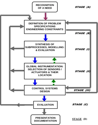
The general features of the technological stages of the overall system design are briefly considered first and are summarised by the diagram of Figure (1). The exchange of information illustrated in the above diagram between the different design stages has a short prediction horizon, as far as the impact on the subsequent design stages, and it is of a local character. This local character is dominated by the specialised skills, theory and techniques needed for a given engineering task. The ability to translate local decisions as actions assigning certain structure to the stage model is currently missing. The common engineering practice is dominated by heuristics, simulations, trial and error and final testing on a pilot plant. Accelerating the design process is crucial and this may be helped by developing a Global Coordination Theory for the design process. Our attention is focused on the technological stages of design, that is:

STAGE (I) : Process Synthesis

STAGE (II): Overall System Instrumentation (Global Instrumentation)

STAGE (III): Control Design.

RECOGNITION OF A NEED

DEFINITION OF PROBLEM SPECIFICATIONS ENGINEERING CONSTRAINTS

SYNTHESIS OF

SUBPROCESSES, MODELLING: & EVALUATION

GLOBAL INSTRUMENTATION: SELECTION OF SENSORS /

ACTUATORS & THEIR LOCATION

CONTROL SYSTEMS DESIGN

EVALUATION

PRESENTATION

DOCUMENTATION STAGE (D)

STAGE (C) STAGE (III)

STAGE (II) STAGE (I) STAGE (B) STAGE (A)

[image:5.595.153.471.356.761.2]

Such a procedure is iterative and it is the result of the technological complexity of the engineering task that requires specialisation. The process synthesis – global instrumentation - control design stages have a cascade nature with feedback loops between the various sub-stages. The cascade nature of design is underlying the evolutionary process of model shaping, that drives the integrated design paradigm (Karcanias,1995a, 2000). The main inputs at every design stage are the special skills, knowledge, local objectives and specification and the model of the previous design stage. Secondary inputs are provided by the exchange of information between the given stage and the other design stages, whenever they exist. The cascade design process is dynamic in the sense that what it is feasible to achieve at a given stage is influenced by the decisions taken at the previous design stages. It is thus a characteristic feature of the cascade design process that decisions taken at one stage, which may been seen as technically reasonable and economically sound according to local criteria, may, not necessarily be good as far as the overall design process. In fact, the overall system tends to display behaviour that is not an aggregate of partial behaviours, but a gradual evolution, expressed in terms of model, properties and respective behaviour. Understanding this evolution of the system and its properties as we go through the successive design stages is crucial in developing the tools for managing this evolution and thus contribute to the development of a Global Coordination Theory (GCT) (Karcanias, 2000) that is crucial for addressing systems integration of complex modern designs.

The formation of structural characteristics of the overall process is reminiscent of an evolution process. The first stage, the process synthesis, acts as the parent gene and thus predetermines a possible range of key characteristics of the final process. Decisions on the successive design stages, contribute to the gradual shaping of the final model structure, however, within a range of possible options and correspond to a sequence of successive mutations. Structural properties evolve, but not in a simple manner. Ideally, we would like to have assigned certain desirable characteristics to the model of every single design stage and thus finally guarantee the shaping of a process with specified properties. This requires perfect control of the model evolution process; however, not all activities may be modelled and what is desirable as final design is impossible to predict at the beginning of each design stage. A more feasible design philosophy is to direct the model evolution process towards final designs that may possess some desirable properties and avoid the formation of undesirable features that may penalize the final control design. This methodological framework is specialised to the design stage of process synthesis and global instrumentation considered below.

Process Synthesis: This is an act of determining the optimal interconnection of processing units, as well as the optimal type and design of the units within a process system. The structure of the system and the performance of the process units are not determined uniquely by the performance specifications. The task is then to select a particular system out of the large number of alternatives which meet the specific performance specifications. Some of the basic problems in Process synthesis are (Morari & Stephanopoulos, 1980), (Morari, 1992): (i) The Representation Problem, (ii) The Evaluation Problem, (iii) The Strategy Problem. The first deals with the question of whether a representation can be developed, which is rich enough to allow all alternatives to be included. The second deals with the question of whether the design alternatives can be evaluated effectively, so they may be compared. The final problem deals with whether it is possible to locate quickly the better alternatives without totally enumerating and testing all options. Problems (i) and (iii) heavily depend on the specific applications domain. Systems and Control provide generic results which can be used to formulate alternative approaches based on generic concepts and these will be considered subsequently.

Global Instrumentation: This deals with the selection of the set and the distribution of inputs and outputs and its study revolves around the investigation of a number of fundamental system type problems. The traditional instrumentation of a process (referred to as “micro”, local aspect) deals with the problem of measurement, or implementation of action upon given physical variables. When however we move from the single physical variable to the classification of internal variables and then the selection of sets of measurement variables (outputs), and actuation variables (inputs), this role changes; we then move from the physical layer to a systems level that is referred to as a “macro” (global) aspect of the instrumentation. The “micro” role of instrumentation (Finkelstein & Grattan, 1994) has been well developed and deals with instrumentation theory and practice. The “macro” aspects (Karcanias, 1994a) of instrumentation stem from that the selection and classification of system variables into inputs and outputs expresses the attempt of the “observer” (designer) to build bridges with the “internal mechanism” of the process in order to observe it and/or act upon it. What is considered as the final system, on which Control System Design is to be performed, is the object obtained by the interaction of the “internal mechanism” and the specification of the overall instrumentation scheme, which plays a critical role in specifying many of structural characteristics of the final system model that determine the easy, or difficult nature of the control design problem. The model evolution at this stage and the implications on the shaping of structural characteristics is an issue with a distinct control theoretic context and it will be examined subsequently.

the mechanisms of model structure formation in the early stages of design is challenging and introduces new problems. The following forms of evolution in design are considered:

(a) Design Time Evolution from “early” to “late” design stages

(b) Numerical Dependent Evolution and model accuracy.

(c) Cascade Design from Process Synthesis to Global Instrumentation. (d) Physical Growth, or Lifecycle Evolution.

The first notion of model evolution is linked to the general procedure in design, where we have a fixed interconnection structure, but at the early stages we require simple modelling for sub-processes and physical interconnections; at the late stages of design more detailed, full dynamics models are required for sub-processes and physical interconnection structures. Here, we observe an evolution of the given structure of the system in the design stage time axis and this problem expresses the Early-Late Design Variability of Model Complexity and corresponding accuracy (Karcanias, 1995b). The second type is linked to the level of numerical accuracy of the model that is used and it refers to the corresponding evolution of predicted properties for the respective model families. The third form of evolution is clearly connected to the cascade nature of the design process. The fourth form is linked to the physical growth, reshaping of the system during some re-engineering in response to different demands and it is a form linked to lifecycle issues.

3. Modelling in Early-Late Integrated Design as an Evolutionary Process

The problems posed here arise in different fields of engineering, and most predominantly in chemical processes (Douglas, 1988), (Rijnsdorp, 1991), (Stephanopoulos, 1984) where there is a need to visualise a complete design of the system, or many possible alternative designs at very early stages, evaluate them in some way and then select the most promising one for further elaboration. These imply that we need: (i) Methods for generating simple models from specifications and appropriate conceptualisations (Representation); (ii) Ability to create nests of models as we proceed from early to late stages that evolve within a physical structure and increase in complexity (Structured Variable Complexity Nesting) and accuracy; (iii) Methods to evaluate full model features and properties on simple early forms (Early Property Prediction); (iv) Theory to explain evolution of system properties as a function of model complexity (Property Evolution). The current practice is dominated by heuristics and little theory. There is need to formalise these unstructured problems in a way that will enable formal methods to be used and appropriate concepts and tools to be developed. These issues are considered in this section and representative problems will be defined.

3.1 Early Models and the Design Time Evolution Nesting

A special form of system evolution is linked to the need for variable complexity modelling (VCM) in the design process as we move from early to late design. In fact, by assuming that we have a fixed interconnection structure throughout the design, then at the Early Stages we require simple modelling for sub-processes and physical interconnections, whereas at the Late Stages of design more detailed, full dynamic models are required for both sub-processes and physical interconnection structures. The study of such problems requires the development of a framework that permits the transition from simple graphs to full dynamic models and allows study of Systems and Control properties in a unifying way. In the following, Process systems are used as the motivating example. For such systems a fundamental stage in the design process is the problem of Conceptual Modelling. This transforms Requirements and Objectives to sets of Preliminary Designs referred to here as conceptual process flow-sheetsic and the procedure is described in (Douglas, 1988), (EPIC, 1989). For Chemical processes, this is done by experienced Chemical Engineers and the overall set of such models is denoted by:



c



i

= , i 1,2,....,k

M M where the basic elements in modelling are:

(i) The general interconnection rule defining the associated graph. (ii) The early description of sub-processes in terms of simple models.

The exact nature of the graph depends on the stage of the design (early, late) and this is affected by the nature of models for local processes and the description of the physical interconnection streams. We may define the following notion of a graph associated with the system:

Definition (3.1): Let us denote every subsystem

Σ

i by a pair of vertices

(

e

i

,w

i

),

denoting inputs and outputs, and an

edge gi providing an input-output description of

Σ

i

.

If we denote by

fik

the physical (information) streams connecting

the

w

i output and the

e

kinput, the set {

(

e

i

,w

i

),

g

i

, f

ik



i, k=1,2,…,μ} will be called the kernel graph of the system.

variability from 1-dimensional vertices, edges to many dimension vertices, edges respectively describes a form of evolution defined as Dimensional Variability of Graphs. Fundamental issues related to the dimensional variability of the graph relate to the classification of the properties of the directed graph, which are independent/dependent on the dimensionality of the corresponding nodes.

Starting from the kernel model, we may develop models of increasing complexity, generated from the same c model.

This is done by preserving the generic structure of the interconnection rule, the kernel graph, and successively using models with increasing complexity for the sub-process. This leads to the following nested set of models:

M

C



M

₀C



M

₁



M

₂



...



M

_K



M

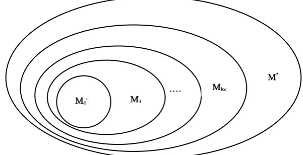
(3.1)

Figure (2): Nested set of models of variable complexity

Clearly, the process of model building continues beyond the construction of o, which is the simplest nonlinear model. This nesting described expresses an evolution of the overall system model, parameterised by complexity (McMillan degree for linear systems) which is due to the evolution of dynamic richnessof the subsystem models and it is due to the time dimension (Early–Late) of the design process referred to as Design Time Evolution.

If



denotes the Graph of c and we denote by



a



i, i 1,...,μ

M the aggregate of the simple models of the a-stage,

we can denote by a, the model defined as:

M

a

 



diag



M

_ia

:i 1,...,μ





. As model complexity for subsystems increases, we may also consider issues of dimensional expansion and/or evolutionary expansion of the corresponding graph (vertices, edges expansion). The latter implies that scalar nodes and edges in a graph may become vector nodes and vector edges and this represents a Dimensional Graph Evolution form. Instead of assuming a fixed



as above we may assume a set

 



and for every





 



we define a



a



i

diag

:i

1,...,μ

 



M



M

with



satisfying

the graph evolution:



₀



₁



₂....



_k 



* (3.2)

The above nesting expresses the progressive enrichment of the initial graph that may be due either to increased local model complexity, and/or due to enhancement of description of the physical interconnection streams (dimensional expansion of graph branches). Such changes express distinct forms of evolution in the overall model and raise important new issues referred to as graphevolution; the resulting nesting of models is denoted in Figure (3).

Figure (3): Model Embedding Process

k

*

....

1

0c

Evolution of

Models in Early

Design

Graph + Nonlinear models

Graph + Full Linear

model Graph + Steady

state models

Conceptual Model =

Graph + Conceptual

representation

Graph + First Order models

[image:8.595.60.537.142.306.2] [image:8.595.182.483.588.742.2]

This problem has two different variations: (i) We adopt a procedure for simplification of description of subsystem models by using Model Reduction, while we preserve the Graph Structure. (ii) We assume a fixed input, output structure for the subsystems and examine the graph variability by using input-output models for subsystems while preserving the kernel graph structure of interconnections. Either of these two processes generates the sequences of models:

M

₀a



M

₁a



M

₂a



...



M

_ka



M

_{k 1}a_



M

_{k 2}a_



...

(3.3)

where

M

₀ais the kernel model,

M

₁a is the linear steady state model,

M

₂a corresponds to first order dynamics,

a k 1

M

may be a nonlinear model with simple Voltera description,

M

_{k 2}a_ the nonlinear model with double Voltera description (Sastry, 1999) etc. Note that there is a reversibility of the model complexity evolution and model simplification approach. Model Evolution and Model Reduction may become completely reverse processes, if we use fixed input, output subsystem structures and interconnection graphs. This expresses a form of duality between model reduction and model complexity evolution. Important research tasks that emerge are:

Complexity Nesting Problems: For the problems of Early Design models the following problems are open:

(a) Describe the mechanisms of nesting by developing appropriate representations for graph evolution, measures for model complexity, and appropriate representation for overall model embedding.

(b) Study the evolution of properties and structural characteristics in the evolutionary ordering of the Composite System Models and classify system properties according to:

●

Invariance, or dependence of the stage model and on early, or late appearance of property in the nesting.

●

Study and clarify the evolution of properties and structural characteristics in the evolutionary process.

■ Challenging tasks are the representation of such forms of evolution, the simplification of graphs (in some sense), defining general measures of model complexity beyond the family of linear models, and linking complexity, and genericity of system properties etc.

3.2 The Model Environment of Integrated Design

The characteristics and nature of Process Synthesis and Global Instrumentation depend on the type of available models and this is referred to as the “Model Environment” of the problem. Note that Instrumentation follows the Process synthesis, but it may be considered at the early stages, when the models are simple and rough, but also at the late stages, when detailed models are available. We may have models where some of the internal variables are classified into potential inputs, outputs, internal variables and referred to as oriented models, or models where no classification has been made of the internal variables and are called implicit models. All such models may be used for selection of effective sets of inputs and outputs, they are referred to as progenitor models and they may be classified as:

● Internal Models (IM) ● External Models (EM)

● Internal-External Models (IEM)

(i) Internal Models (Lewis, 1989): These are described in terms of first order ordinary nonlinear equations and they are the standard state space descriptions of the implicit type

g

(



,





)



0

, where is the vector of all internal model variables. In the linear case, the above reduces to matrix pencil model (Karcanias & Hayton, 1982) defined by

F G



(3.4)

When the inputs

u

, outputs

y

have been defined, then

y



h

(



,

u

)

,

q

(



,





,

u

)



0

is the nonlinear model, which in the

linear case becomes the singular model

E



A



B

u







,

y



C



(3.5)

When we have higher order derivatives, then autoregressive descriptions are used (Willems, 1989).

(ii) External Models (Vidyasagar, 1981): If



,



denote the spaces of all potential inputs, measurements, referred to as extended input, output spaces respectively and

v, z

are the corresponding p, q-dimensional vectors, then the external, or input-output map

f

is a function

f

:

V



Z

where

z



f

 

u

. For the case of linear, time invariant

systems

f

is a convolution function, or it is represented by the q



p rational transfer function matrix

F

 

s

, for which

Note that



,



denote the potential input, output spaces and not the effective ones, which are denoted by



,



and have corresponding dimensions ,

m

. If

u, y

are the effective input, output vectors, and if

H, Q

are representations of the sensor, actuator maps, then

y s

 



H z s

 

,

v s

 



Qu s

 

and the effective transfer function is:

W

 

s



H

F

 

s

Q

(3.8)

(iii) Internal-External Models: A large process is always synthesised by connecting sub-processes and the two fundamental ingredients of the composite system model are: (a) The topology (graph) of system interconnections

F

, represented by a matrix

F,

and (b) The family {} of subsystem models which may be of any of the types discussed before. If



_a denotes the aggregate (direct sum) of the sub-processes and

F

the graph interconnection rule, then



_c



F





_a (3.9)

represents the composite system model and a feedback type representation will be given in the next section. For the linear case

Σ

 may be represented as a diagonal of transfer functions, and thus

Σc

becomes also a transfer function with a specific structure.

3.3 Prediction and Evaluation of Overall System Properties in Early Models

The development of the family of early design models is integral part of the need to evaluate properties of the final system at early stages and thus avoid taking roots that may lead to bad designs. In the context of Chemical Processes this is usually referred to as process controllability and operability studies (Douglas, 1988), (Perkins, 1990), (Morari, 1992). Process Controllability is a generic term which does not carry the same meaning as that used in mainstream system and control; usually, it is interpreted as the ability to operate despite the affect of disturbances, ability of the designer to achieve performance requirements after implementation of a suitable control scheme etc. As such, Process Controllability (contrary to the linear systems notion of State Controllability) is a term that requires an exact definition of its meaning. Operability also has a quite diverse meaning and it is linked to issues such as: Product, Input Driven Flexibility (material variability), Recoverability (Ability to drive the process back to safety after faults), maintainability etc (Perkins, 1990), (Morari, 1992). The variety of alternative structures (process flowsheets) generated at the early stages of design have to be evaluated with a variety of criteria. There have been two main schools of thought (Rijnsdorp, 1991):

Ideal Evaluation: Assess the behaviour of a system with a controller of specified complexity, which is tuned optimally. Realistic Evaluation: Development of low effort analysis tools giving a reasonable indication of the quality of closed-loop behaviour allowing the designer at least to rank and order alternatives according to controllability, operability etc.

The first requires a complete system (with instrumentation and Control) and it is rather unrealistic (although scenarios based on models may be deployed). The following properties are important in such evaluations:

Flexibility:Is defined as the ability of the system to handle a new situation at steady-state and thus express the ability to operate at different steady states.

Switchability: Considers ability of a plant to be moved from one steady state operating point to another. This also involves start up and shut down of the process.

Controllability: Is the “best” dynamic performance (set point following and disturbance rejection) achievable for a system under closed loop control.

Safety: Examines the hazards that may be involved with particular designs and using process dependent heuristics provides a classification.

The above key properties for the evaluation are emergent system properties and express aggregation of structural system and controller dependent features of the family of models. Process Controllability is a much more general notion than the traditional system controllability, Flexibility depends mainly on the structure of the process, whereas “Switchability” and Controllability depend on the system structure and the selected control structure (Morari, 1992). The available tools for such studies are mostly heuristic and there is need for a Systems and Control framework for characterising these properties.

Control Based Characterisation of Design Emergent Properties: Develop a systems and control type framework for:

(i) Interpretation of Evaluation Criteria for Process Synthesis;

(ii) Prediction of Full Model System Properties based on early simple models.

The exact System and Control context of these emergent properties is not specified, and thus they are not structurally interpretable in terms of values, properties of design indicators, invariants etc. Specifying exactly the meaning of all such properties is essential prerequisite for the Control theoretic evaluation of the alternative process structures. The prediction of full model properties benefits from the knowledge gained in (i) and the understanding coming from the model structure evolution. So far, there is no control theoretic framework for such problems with few exceptions the conditioning of early design models (Karcanias & Vafiadis, 2001) considered subsequently. A feasible approach is to use simple models, assume that global instrumentation delivers the best possible final structure and then try to establish criteria predicting the fundamental system properties on the final system that will emerge.

3.4 Well conditioning of Early Design Models

The development of models, which may be used for evaluation of alternatives is an integral part of the Early Process Design of process plants (Douglas, 1988). Such models are usually developed for the entire plant, are based on the selected process flow-sheet and involve the use of simple models of the sub-processes. They are large dimension models and their final structure is determined when the control structure is decided. This problem involves a number of key issues of system theoretic nature and they are considered here. It is assumed that a linear model of a system is given with given inputs and outputs. At the early stages of design it is desirable to include as inputs, and outputs all possible variables that can be used which may play the corresponding role; such sets are defined as potential inputs,

potential outputs respectively. The model that corresponds to the potential inputs, outputs provides the basis for deriving all subsequent models based on effective input, output sets and it is thus referred to as the progenitor model.

For such models, all inputs and outputs are physical variables that can be controlled and measured. At a later stage, when we proceed to control design, the number of effective inputs and outputs requires reduction. This reduction implies an appropriate selection of rows, columns of the transfer function matrix, or the corresponding system matrix such that the corresponding subsystem has desirable properties.

Progenitor models involve all potential inputs and outputs and they may have structural undesirable properties that do not allow their effective use in design. In fact, a progenitor model may be structurally degenerate (Rosenbrock, 1974), might have redundancy in the input, output schemes, may be uncontrollable/ unobservable and may have high order infinite zeros. A progenitor model represents all our knowledge about the system at a given stage of early design and the McMillan degree of this transfer function represents the natural order n of the system. System models, which are degenerate, do not satisfy the basic condition of the output function controllability (Rosenbrock, 1970). It is thus desirable to select subsets of the potential inputs and outputs, such that the resulting transfer function is “well-conditioned” in some sense. Systems which are well-behaved are referred to as well-conditioned system. Amongst the basic criteria used, are the properties of non-degeneracy, controllability and observability of the system model and non-redundancy of the input and output scheme. The problem considered here, is the use of the characterisation of the above system properties to develop a parameterisation of all possible systems corresponding to effective inputs and effective outputs by selecting appropriate sub-sets of the potential variable sets (Karcanias & Vafiadis, 2001) and which are well behaved in some specified sense.

It is assumed that the progenitor model is described by the minimal state space equations for

S(A,

B,

C,

D)

:

n n

n r

x A x B u , A









, B





y C x





D u , C



q n



, D



q r



(3.10)

with a transfer function

H(s)



qxr

(s)

and



= rank(s)

{

H(s)

}.

Clearly (Karcanias, 2002), if <min(q,r), then the system

is degenerate, and if = min(q,r), it is non-degenerate.

Remark (3.1)(Rosenbrock, 1974):  defines the maximal number of output variables that may be controlled independently (output function controllability criterion) and the minimal number of independent inputs required to control  outputs.

■ If r, q ≤n, and define: r = rank{[B

t

,Dt]} ≤ r,  = rank{[C,D]} ≤ q, then if r < r, (< q ) the system will be said to have

input (output) redundancy; otherwise, i.e. if r = r, (= q ), it will be called regular. Regularity of the model is equivalent

to non-redundancy of both sensor and actuator schemes. The well conditioning problem corresponds to selection of subsets of potential inputs and outputs; thus, it is equivalent to deriving a smaller transfer function H(s) from H(s) by eliminating sets of rows and columns, such that H(s) has certain properties. Important issues are:

Well Conditioning of Progenitor Models Problems:Given the progenitor model described by H(s), or with a minimal realization S(A,B,C,D), define subsystems S(A,B,C,D) by selection of subsets of inputs and outputs such that:

(i) S(A,B,C,D) have the maximal cardinality subset of the potential input and output sets, the resulting transfer

function is non-degenerate, it has the maximal possible normal rank and it is also proper.

■

The solution of problem (i) is referred to, as well-conditioning of Progenitor models and part (ii) describes the property that the resulting model is both controllable and observable. Note that controllability and observability are notions defined on S(A,B,C,D) where A corresponds to the minimal realisation of H(s). The latter problem will be referred to as normal-conditioning of Progenitor Models. Note that the above problems involve the study of properties of the sub-matrices of the rational transfer function matrix H(s) obtained by elimination of certain sets of columns, rows.

The notion of degeneracy has been classified into a simple form when there is redundancy of the input, output map of the progenitor model and to a structural type referred to as strong which is linked to internal properties of the system. The distinction between the two types is based on the zero- nonzero values of associated minimal indices of the transfer function. Criteria have been given for the presence of input, output redundancy, strong degeneracy, lack of minimality (based on Hankel matrix tests) (Antsaklis & Michel, 1997), and high order infinite zeros (Karcanias, 2002). Procedures have been suggested on how such properties can be avoided and searching techniques for defining sub-systems with maximal input, output cardinality which are also well conditioned, have been given (Karcanias & Vafiadis, 2001), based on the notion of natural bases of matrices (Karcanias and Mitrouli, 1998) and use of Grammians (Gantmacher, 1959). The results have led to parameterisation of all subsystems, which are input-output regular, nondegenerate, minimal and have maximal cardinality (r~,q~)(Karcanias & Vafiadis, 2001).

3.5 Structural Identification

The study of system properties based on well defined models is a well established activity. However, at the early stages of design, models are characterized by structural and parametric uncertainty and this makes the study of system problems on so called “ill-defined” models a challenging problem (Karcanias et al, 1996). Features such as high dimensionality, uncertainty in system parameters and constraints of information structure often lead to problems, which cannot be solved using traditional methods developed for well-defined models. At the early stages of design we would like to have some insight into the structure of the system, and more precisely into general properties, such as possible value of McMillan degree, controllability, observability, existence of fixed modes, high order infinite zeros etc, even on models which are not precisely defined. These properties may be regarded as “potential” system properties, characterize, or enter the solvability of control synthesis problems. Ideally we would like to be able to predict the true system properties of the full model from the properties of ill-defined models, which are available at the early process design stage; this is equivalent to predicting properties and structure on the fully evolved model. Special classes of system models for which some results have been defined are those characterized by:

(a) Certain general parameters, such as the number of inputs, outputs, states are fixed, but otherwise having generic values for their parameters and referred to as Fixed Order Generic Systems (FGOS).

(b) The interconnection graph is known and the subsystems are represented by fixed dominant dynamics, or fixed relative order of the entries of the transfer functions, but still have uncertainty in the remaining parameters; these are referred to as Structured Dominant Dynamics Systems (SDDS).

Representative models in the SDDS class are the Structured Transfer Functions (STF) models which have certain elements fixed to zero, some elements being constant and other elements expressing some identified dominant dynamics of the system, or having fixed relative order of the entries of the transfer functions. Structural properties are generically possessed by all systems that may have different parametric values, but share the same underlying graph structure, or fixed structural features. Computing structural invariants on such families of uncertain models by using genericity arguments and exploiting the underlying structure, is referred to as Structural Identification; these problems include the evaluation of structural characteristics on state-space or transfer function models, such as minimal indices (controllability, observability, Forney indices, etc.) and invariant zeros. For such structured models the evaluation of certain system properties (Karcanias, 2002), (Karcanias & Vafiadis, 2002a) involves graph theory (Reinschke, 1998) and computations may be reduced to optimization problems on integer matrices (Karcanias et al, 2007). The properties that have attracted most of the attention for such systems have been the evaluation of the generic McMillan degree (Karcanias et al, 1996), (Van der Woude, 1995) and the generic infinite zero structure (Vardulakis et al, 1982), (Hovelaque et al., 1997). A promising approach for such computations is to use the genericity argument and this reduces the problem to study of properties of “weight” of integer matrices (Karcanias et al, 2007).

Definition (3.2): Given a matrix

A



m n we define: (i) A

k

-length independent path

1 1 2 2

{

,

,

,

}

k k

i j i j i j

a

a

a

, as a set of

elements from the matrix such that

a

i j 

  

0,



1,

,

k

and there is no common index in the sets

{ , ,

i i

1 2

, }

i

k and

1 2

{ ,

j j

,

,

j

_k

}

. (ii) The weight of a path is the sum of the elements of the matrix that belong to the chosen path. (iii) The maximal weight of all the independent paths of a matrix

A

is denoted by γ(

A

) and it is simply referred to as the

weight of the matrix

Determining the “weight” of integer matrices is equivalent to “optimal assignment problems” in operational research (Bertsekas, 1981), (Sagianos, 2008). The development of fast and reliable computations for the generic values of structural characteristics on the family of early models is a challenging task. An efficient computational procedures using the notion of reducibility of integer matrices for finding solutions to “optimal assignment problems” has been developed in (Karcanias et al, 2007).

3.6 Model Nesting and the Issue of Small Numbers

For linear state-space, or transfer function models, the issue that often arises, is how to handle numbers, which are very small and what is the impact of rounding off certain numbers of order less than a given order on the structural properties. It is essential to make a distinction between numbers which are small enough to be assumed equal to zero, and thus do not affect the overall structure of the system, or any of its properties, and numbers which are small, but represent a coupling, which has to be preserved. The small numbers, appearing in the A, B, C and D matrices, or in the set of Markov parameters {D, CB, CAB, CA2B, …} may be classified into structural which affect structural properties and non-structural, the removal of which has no effect on system properties. This classification introduces a numerical form of model nesting (Karcanias & Sagianos, 2008). Removing small numbers is a form of Robust Structural Simplification, given that the structural properties of the original system have to be close to those of the reduced system.

Consider a state-space model

(

A B C

 

)

and let

r

be the element of maximal absolute value in

(

A B C

 

)

. We can

define the scaled model

(

A B C

  

 

)

as:

1

0

0

A

B

A

B

P

C

C

r







 



 

_

_{ }



_





 



(3.11)

For the elements of

P



we have clearly

0



p

_ij

 

1

If





0

is any small number, then all elements of

P



for

which



p

_ij





defines a set, that will be called the





power of the original system. According to the value we

select for



we have a new model, the





simplified model, which is defined by the matrices

A B C

_

  

_{ } or

A

_

  

r A B

_{ }

 

r B

_ and

C

_

  

r C

_ The Boolean matrices associated with the





simplified model, will define

the





structured model denoted by

{ }

P

_.

Robust Structural Simplification Problem: Different methods can be used to decide on the significance of the value of



and the final form of the





structured model

{ }

P

_. Amongst the possible methodologies we can use to analyse the effect of small numbers on the system properties are (Sagianos, 2008): (i) Sensitivity Analysis Approaches; (ii) Robustness of Graph Structures; (iii) Degree of Controllability and Observability; (iv) System Based Metrics and Properties; (v) Matrix Perturbation Theory. All these methodologies adopt the same philosophy, which is to evaluate the effects of the different



we choose on the structural properties of the system.

▀

Consider a linear system represented by a state-space description

S A B C D

(

  

),

or by the set of Markov Parameters



(

H H H … H

₀

 

_{1 2}

 

_n1

 

…

)

We assume that the elements in the matrices involved are known only in terms of their relative order, but they are otherwise generic. This may be defined precisely as follows: Consider the set of positive real numbers

{

a a a … a

₀

   

_{1 2 }

}

such that

a

₀

 

a

₁

a

₂

 

… a

_ and define the following intervals:

E

₀

 



,

a

₀





E

₁





a a

₀

,

₁





E

₂





a a

₁

,

₂



,...,

E

_





a

_1

,

a

_

_





E

_1





a

_

, 0



_

(3.12)

Definition (3.3): Let

M



R

m n and assume that the order of its elements (absolute values) are known only in terms of their membership of the sets

E

₀



E E

₁



_



...,

E

_1, but they are otherwise generic. Such a matrix

M

will be called

0 1

{

a a … a

  

_

}

-structured generic matrix (ie

a

₀



10

2

 

a

₁

10

3

 

… a

_



10 )

6 and the set of such matrices will be denoted by

0

m n a …a

R





 



For any matrix 0 1

m n a a …a

M

R



   



we may:

M

₀: is obtained from

M

by setting all elements which are not in

E

₀ equal to zero.

M

₁

M

by setting all elements which are not in

E

₀



E

₁ equal to zero.

. .

M

_: is obtained from

M

by setting all elements which are in

E

_1 equal to zero, or equivalently all elements not in

E

₀

  

E

₁

… E

_ equal to zero.

▀

The above process creates from

M

a set of matrices

M M M … M

₀



₁



₂

 

_ which together with

M

define a nesting condition denoted by

0 1 2

M



M



M

 

… M





M

(3.13)

The relation “



” means that

M

_ is obtained from

M

_{ 1} those elements of

M

which have an absolute value in the interval



a

_1



a

_





This ordering on the

M

matrix will be called an

{

a a a … a

₀

   

_{1 2} 

}

-induced nesting and this

numerical nesting leads to families of State Space and Markov Parameter Nested Models which may be denoted by

{ } =

S



S A B C D

j

(

j

  

j j j

), j=1,2,....,



(3.14)

{ } =



_



_j

(

H

j₀



H

j₁



H … H

j₂

 

j_n1



…

), j=1,2,...,



(3.15)

Structural Numerical Model Embedding Problem: For the families

{ }

S

,

{ }



systems investigate:

(i) The minimal value of the order ε required for the emergence of different system properties, such as controllability, observability, stability etc. in either of the two families.

(ii) How the McMillan degree varies as a function of the in the family

{ }



_in terms of ε

(iii) Whether properties established for a certain ε are preserved in models of higher accuracy ε. (iv) Theexistence of properties which are dependent, or independent on the selected value of ε.

▀ Note that the state space modelling and the input-output modelling based on the Markov parameters provides different

approaches for the study of robustness and sensitivity. The Markov parameters approach is naturally linked to the partial realization problem (Kalman,1979), (Antoulas etc, 1991) and this in turn implies some further evolution of structural properties based on the predicted McMillan degree of the partial realization (Sagianos, 2008).

4. Process Synthesis as a Generalised Feedback Design Problem

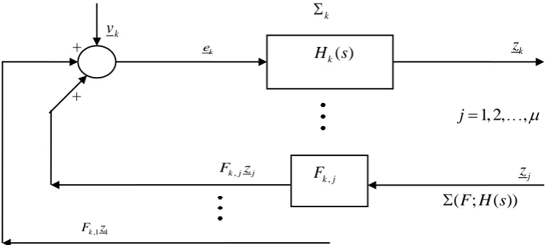
The problem of process synthesis is usually addressed using methodologies linked to the specifics of the application area. The development of a generic synthesis framework that transcends the different application areas is a significant challenge. The modelling of composite systems using energy considerations, or behaviours (Willems, 1997) and the use of the traditional network synthesis together with the completion of the analogy between electrical and mechanical domains (Smith, 1995) are important contributions. In this section, we explore an alternative idea that relates to the reduction of process synthesis to an equivalent feedback design problem using the standard composite system description (Callier & Desoer, 1982) and its particular characteristics based on the nature of the physical interconnection streams and the selection of the local input and output structure (Karcanias, 1995a). This work introduces an important notion of completeness (Karcanias, 1996) and provides a representation of the synthesis as generalised feedback design problem. Such representation provides the means to intervene with systems and control tools in a design area which is dominated by the specifics of the application area. If {

Σi,

i} is a set of subsystems with models {



i, i} of a certain type and if



is the interconnection rule (described by a graph), then

a 1 2 μ

Σ



Σ Σ

  

Σ

denotes the aggregate system with a model

M

_a



block diag





M

₁

,

M

₂

, ...,

M

_μ



. The

Composite System is denoted by

Σ

_c

 



Σ

_a, where * denotes the action of



on

Σ

_awhich will be subsequently defined.