Poly: A Reliable and Energy Efficient Topology Control Protocol for Wireless Sensor Networks

City, University of London Institutional Repository

Citation

:

Qureshi, H. K., Rizvi, S., Saleem, M., Khayam, S. A., Rakocevic, V. and

Rajarajan, M. (2011). Poly: A Reliable and Energy Efficient Topology Control Protocol for

Wireless Sensor Networks. Computer Communications, 34(10), pp. 1235-1242. doi:

10.1016/j.comcom.2010.12.016

This is the accepted version of the paper.

This version of the publication may differ from the final published

version.

Permanent repository link:

http://openaccess.city.ac.uk/15289/

Link to published version

:

http://dx.doi.org/10.1016/j.comcom.2010.12.016

Copyright and reuse:

City Research Online aims to make research

outputs of City, University of London available to a wider audience.

Copyright and Moral Rights remain with the author(s) and/or copyright

holders. URLs from City Research Online may be freely distributed and

linked to.

City Research Online:

http://openaccess.city.ac.uk/

[email protected]

1 2 3 4 5 6 7 8 9 10 11 12 13 14 15 16 17 18 19 20 21 22 23 24 25 26 27 28 29 30 31 32 33 34 35 36 37 38 39 40 41 42 43 44 45 46 47 48 49 50 51 52 53 54 55 56 57 58 59 60 61 62

Poly: A Reliable and Energy Efficient Topology

Control Protocol for Wireless Sensor Networks

Hassaan Khaliq Qureshi

_{, Sajjad Rizvi}

_{, Muhammad Saleem}

_{, Syed Ali Khayam}

_,

Veselin Rakocevic

and Muttukrishnan Rajarajan

∗_{School of Electrical Engineering & Computer Science (SEECS)} National University of Sciences & Technology (NUST), Islamabad, Pakistan.

Email:{hassaan.khaliq, sajjad.rizvi, ali.khayam}@seecs.edu.pk

†_{School of Engineering and Mathematical Sciences, City University, London, UK.} Email:{hassaan.qureshi.1, V.Rakocevic, R.Muttukrishnan}@city.ac.uk ‡_{Center for Advanced Studies in Engineering (CASE), Islamabad, Pakistan.}

Email: [email protected]

Abstract—Energy efficiency and reliability are the two

impor-tant requirements for mission-critical wireless sensor networks. In the context of sensor topology control for routing and dis-semination, Connected Dominating Set (CDS) based techniques proposed in prior literature provide the most promising efficiency and reliability. In a CDS-based topology control technique, a backbone – comprising a set of highly connected nodes – is formed which allows communication between any arbitrary pair of nodes in the network. In this paper, we show that formation of a polygon in the network provides a reliable and energy-efficient topology. Based on this observation, we propose Poly, a novel topology construction protocol based on the idea of polygons. We compare the performance of Poly with three prominent CDS-based topology construction protocols namely CDS-Rule K, Energy-efficient CDS (EECDS) and A3. Our simulation results demonstrate that Poly performs consistently better in terms of message overhead and other selected metrics. We also model the reliability of Poly and compare it with other CDS-based techniques to show that it achieves better connectivity under highly dynamic network topologies.

I. INTRODUCTION

Wireless Sensor Networks (WSNs) are envisioned as an enabling technology for a broad class of mission-critical applications. It is generally assumed that nodes in a WSN are connected to their neighbors with a certain probability of packet loss. Since wireless links are inherently unreliable, these packet losses are not acceptable for many mission-critical WSN applications (e.g., forest fire detection, battle field monitoring) which require the network topology to pro-vide a certain desired level of reliability. This reliability should however be achieved while keeping in mind the fundamental energy consumption constraint of a WSN. In this context, the graph-theoretic Connected Dominating Set (CDS) principle has emerged as the most popular method for energy-efficient topology control (TC) in WSNs [2], [3], [4], [5], [6], [7].

TC consists of two phases: topology construction and

topology maintenance. In the topology construction phase, a desired topological property is established in the network while maintaining connectivity. Once the topology is con-structed, topology maintenance phase starts in which nodes switch their roles to cater for topological changes. In

CDS-based TC schemes, some nodes are a part of the virtual backbone which is responsible for relaying packets in the WSN. Non-CDS nodes conserve energy by turning off their transceivers. CDS size is a critical parameter which controls the compromise between reliability and energy efficiency.For instance, for small CDSs, fewer nodes handle the bulk of the network traffic and consequently deplete their batteries quickly [5]. The positive side of a small CDS is that more nodes can go to sleep mode. While both of these metrics – energy efficiency and reliability – are equally important for mission-critical WSNs, existing CDS-based routing protocols cannot simultaneously cater both metrics [5], [6], [7].

In our earlier work, we analyzed the performance of main-taining a cycle in a 10 node network [17]. However, to understand practical limitations, it is important to analyze the performance on larger networks against other widely available protocols. In this paper, we propose a semi distributed graph-theoretic topology control protocol for wireless sensor net-works. The protocol, referred to as the Poly protocol, models the network as a connected graph and finds the number of polygons present in the network. Based on the duplicate node IDs of different nodes, Poly adaptively finds a polygenic backbone to turn-off the unnecessary nodes while keeping the network connected and covered. To achieve energy efficiency, the protocol forms a CDS like polygenic network which in turn provides reliability in the case of random link failures. Moreover, it adapts to topological changes in the network based on the remaining energy of the nodes. This allows topology maintenance among different set of nodes to increase the network lifetime.

The Poly protocol has a low message complexity which allows the protocol to run multiple times during topology construction and maintenance phases. It can also be applied to different data reporting models which aim to find rendezvous point’s (RPs) and can provide polygenic redundancy to RPs [10]. In addition, Poly achieves energy efficiency while con-sidering network reliability.

1 2 3 4 5 6 7 8 9 10 11 12 13 14 15 16 17 18 19 20 21 22 23 24 25 26 27 28 29 30 31 32 33 34 35 36 37 38 39 40 41 42 43 44 45 46 47 48 49 50 51 52 53 54 55 56 57 58 59 60 61 62

2

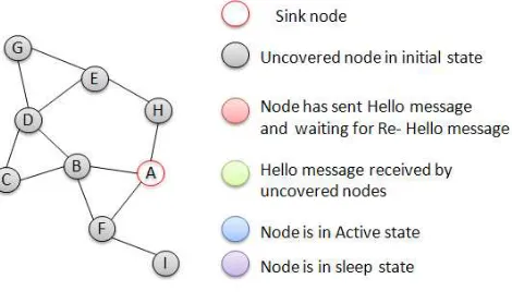
Fig. 1. A sample Network

tocols. Simulations are performed under different underlying topologies, varying node densities to analyze message over-head, energy overover-head, residual energy and network connec-tivity. Simulation results show that the proposed Poly protocol has low energy overhead and it has19%better residual energy when compared with CDS-Rule K protocol. Similarly, it has 32% and34% better residual energy versus EECDS and A3 protocol while performing better under topology maintenance techniques. In addition, the results also demonstrate that Poly is 120% more reliable under varying link probabilities than rest of the competitor protocols.

The rest of this paper is organized as follows. Section II summarizes the background and related work in this area. Section III contains the description of the Poly protocol. We describe the empirical evaluation framework utilized for the performance analysis of Poly in Section IV. Simulation results are provided in Section V. Reliability analysis of Poly is presented in Section VI. We summarize the salient findings of this paper in Section VII.

II. BACKGROUND ANDRELATEDWORK

In this section, we first describe the prominent topology con-struction protocols. In the second subsection, we summarize the topology maintenance techniques which are later utilized to evaluate the performances of different topology construction protocols.

A. Topology Construction Protocols

To achieve energy efficiency, [2] and [11] construct topolo-gies by controlling the transmission power of WSN nodes. Another approach is to make use of geographical location of the nodes [12]. The down side of these approaches is the fact that power control and location awareness are difficult to realize in practical WSN deployments.

An alternative mechanism is proposed in [13] in which a vertex dominating itself and all the adjacent vertices forms a cluster in the graph. A similar Dominating Set (DS) based solution is proposed in [4] which uses the concept of inde-pendent dominating sets. Both of these protocols have led to the concept of Connected Dominating Set (CDS) based topology construction protocols for the generation of energy-efficient topology in WSNs. The authors of [5] have proposed

a topology construction protocol that produces an approximate solution to form a sub-optimal CDS. A3 selects active nodes which are at the farthest distance from the parent based on the signal strength and remaining energy. This allows fewer nodes to be selected in the CDS tree which in turn leads to an overhead of long distance communication.

The authors of [6] have proposed an Energy-Efficient CDS (EECDS) protocol that computes a sub-optimal CDS in an arbitrary connected graph. EECDS uses two phase strategy to find a CDS. In the first phase, a node elects itself as a cluster-head and then all its neighbors are marked as covered in order to find a Maximal Independent Set (MIS). In the second phase, all the covered nodes except the cluster-heads compete to become gateways to form a CDS. In EECDS, nodes maintain the cluster-head role by gathering neighbor information which allows uniform distribution of energy resources. CDS-Rule K, proposed in [7], uses marking and pruning rules to exchange the neighbors lists among a set of nodes. A node remains marked if there is at least one pair of unconnected neighbors and unmarks itself if it determines that all of its neighbors are covered with higher priority. The node’s higher priority is indicated by its level in the tree.

Interestingly, the authors of [8] and [9] have shown that CDS backbones are more vulnerable to node and link failures in WSNs. To this end, they have proposed two approximation al-gorithms – Connecting Dominating Set Augmentation (CDSA) andk-connectedm-dominating set (k, mCDS) – to construct ak-connected virtual backbone which can accommodate the failure of one wireless node. However, they do not analyze the impact of havingk-connected virtual backbone on the energy efficiency of the network.

B. Topology Maintenance Techniques

Topology maintenance is a process in which the network topology is changed / maintained during the lifetime of a network. There are various classes of topology maintenance techniques which can be broadly classified into two cate-gories: static and dynamic. As the name suggests, in static maintenance procedures, all possible sets of topologies are computed off-line / during the initial topology construction process. These topologies are then rotated in a desired fashion. On the other hand, dynamic topology maintenance techniques form a new topology based on the present condition of the network, e.g. as an energy threshold is reached.

Topology maintenance procedures may also be classified on the basis of time and energy triggering mechanisms. In time-triggered methods, topology is rebuilt after a specific period of time. However, these mechanisms are generally expensive in terms of message and energy overhead. Therefore, in this paper, we only focus on topology maintenance based on energy thresholds.

We now explain the working of the Poly protocol in the next section.

III. THEPOLYPROTOCOL

2 3 4 5 6 7 8 9 10 11 12 13 14 15 16 17 18 19 20 21 22 23 24 25 26 27 28 29 30 31 32 33 34 35 36 37 38 39 40 41 42 43 44 45 46 47 48 49 50 51 52 53 54 55 56 57 58 59 60 61 62

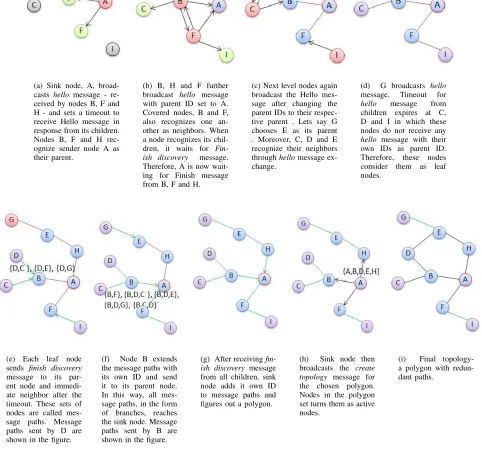
(a) Sink node, A, broad-casts hello message - re-ceived by nodes B, F and H - and sets a timeout to receive Hello message in response from its children. Nodes B, F and H rec-ognize sender node A as their parent.

(b) B, H and F further broadcast hello message with parent ID set to A. Covered nodes, B and F, also recognizes one an-other as neighbors. When a node recognizes its chil-dren, it waits for Fin-ish discovery message. Therefore, A is now wait-ing for Finish message from B, F and H.

(c) Next level nodes again broadcast the Hello mes-sage after changing the parent IDs to their respec-tive parent . Lets say G chooses E as its parent . Moreover, C, D and E recognize their neighbors throughhellomessage ex-change.

(d) G broadcasts hello message. Timeout for hello message from children expires at C, D and I in which these nodes do not receive any hello message with their own IDs as parent ID. Therefore, these nodes consider them as leaf nodes.

(e) Each leaf node sends finish discovery message to its par-ent node and immedi-ate neighbor after the timeout. These sets of nodes are called mes-sage paths. Mesmes-sage paths sent by D are shown in the figure.

(f) Node B extends the message paths with its own ID and send it to its parent node. In this way, all mes-sage paths, in the form of branches, reaches the sink node. Message paths sent by B are shown in the figure.

(g) After receiving fin-ish discovery message from all children, sink node adds it own ID to message paths and figures out a polygon.

(h) Sink node then broadcasts the create topology message for the chosen polygon. Nodes in the polygon set turns them as active nodes.

(i) Final topology-a polygon with redun-dant paths.

Fig. 2. The Poly Protocol

topology construction protocol are: 1) its resultant topology should provide a desired level of packet delivery reliability, and 2) its energy efficiency should be comparable to or less than existing CDS-based topology construction protocols. To satisfy these constraints, the Poly protocol arranges the nodes in such a way that they form a closed path among a set of nodes. The closed path provides a reliable and energy efficient topology because: 1) the sink node gets polygenic

redundancy with its neighbors which allows the nodes to use an alternative path in case of random link failures, and 2) it forms an active node set – nodes comprising a polygon – allowing leaf nodes to enter into the dormant / sleep mode. An additional advantage of polygenic is that the topology construction protocol does not need to position or orientation information of the nodes.

1 2 3 4 5 6 7 8 9 10 11 12 13 14 15 16 17 18 19 20 21 22 23 24 25 26 27 28 29 30 31 32 33 34 35 36 37 38 39 40 41 42 43 44 45 46 47 48 49 50 51 52 53 54 55 56 57 58 59 60 61 62

4

formation process. In the first subsection, we define the type of control messages that are used during the topology construction. Subsequently, we illustrate the mechanism that leads to the formation of polygons in the network.

A. Description of control messages

The Poly protocol uses three types of messages which are involved in the polygon formation process. A hellomessage which contains the parent ID of the sender. Afinish discovery

message which is used by the parent node to announce the end of the topology discovery process. In the finish discovery message, each node sends a list of its discovered neighbors. Finally, acreate topologymessage containing the IDs of active node set is propagated in the network.

B. Topology construction protocol

Topology construction phase of the Poly protocol is divided into three phases. In the first phase, a CDS is created during which the nodes discover their neighbors. The neighbor dis-covery process is initiated by a pre-defined node (e.g., the sink node) and terminates at the leaf nodes. In the second phase, each leaf node sends its neighbor list through the upstream neighbor – the so-called parent node – to the sink node. In the third phase, the sink node discovers polygons in the graph. Subsequently, the polygon nodes are informed that they are part of the active node set. In this way, a closed path is formed with connecting paths to the branches.

We describe the formation of polygon with the help of an example network shown in Figure 1. The Poly protocol starts with an initiator node which in our case is node A. Node

A broadcasts a hellomessage and starts a timer to receive a

helloresponse from its children (see Figure 2(a)). As described earlier, thehellomessage contains the parent ID of the sending node. In the case of the initiator node, this field is empty.

The hello of node A is received by B, F and H nodes located within its transmission radius. These nodes are un-covered nodes which means that they are in the initial state and have not yet chosen any parent node. Therefore, nodes

B, F and H – after receiving the message – choose A as their parent node. The uncovered nodes further rebroadcast the

hello message to discover their children, and also start their respective timers to receive their children nodes’ responses. Every rebroadcasting node, before forwarding the message, updates the parent ID field by replacing it with its own parent ID; for instance, nodesB,F andH in Figure 2(b) update the parent field to the ID of node A.

The rebroadcasthellomessage is also received by the parent node A. Consequently, node A identifies the sender of the

hello message as one of its children. Once identified, nodes

B,F and H are considered ascovered nodes. Furthermore, when a node identifies a child node, it switches to an active state and starts to wait for finish discoverymessage from the children. When the hello message is received by a covered non-parent node, the receiving node identifies the sender as one of its neighbors. For instance, in the given example, the

hello message from B is also received by node F – a non-parent node – leading to the identification of node B as a neighbor of node F. In this manner, the nodes discover their neighbors during CDS creation. and the process is repeated until the network is completely covered (see Figure 2(c)).

The rebroadcast ofhellomessages continues until they reach the leaf nodes e.g. nodes C, D and I in Figure 2. The leaf nodes follow the same process but their timeout expires as these nodes do not have any child node. When timeout expires at leaf nodes, they send finish discovery messages to their parent nodes thereby initiating the second phase of the protocol as shown in Figure 2(d). After sending a finish discovery

message, a leaf node enters the sleep mode and turns off its transceivers to conserve energy. Note that the neighbors of node A do not send any explicit response. Instead, they simply rebroadcast thehellomessage which also functions as a response message for nodeA. Consequently, nodes avoid the use of any explicit response message and reduce the number of control messages exchanged during the topology discovery. In the finish discovery message, each node sends the list of its neighbors to its parent node. In the example, node C

and node E are neighbors of node D. Therefore, node D

sends {D, C},{D, E},{D, G} to its parent (node B) in the

finish discoverymessage (see Figure 2(e)). These sets of nodes create message paths which can then be used for polygon formation among a set of nodes. A node wait for the finish discovery messages from all its children. When it receives all the expected messages, it creates its ownfinish discovery

message and forwards it to its parent node. NodeB in Figure 2(f) extends the received set of message paths with its own message ID. In this way, finish discovery message converges towards the sink node.

When the sink node has received finish discoverymessage from all of its children, it combines different message paths to discover polygons in the network. If there are at least two common nodes in the two message paths, then a polygon exists in the network. For instance,{A, B, D, G} and{A, H, E, D}

are two message paths and have two common nodes A and

D. Hence, it can be inferred that there exists a polygon in the network comprising nodes{A, B, D, E, H, A}(see Figure 2(g)).

Figure 2(h) shows the selected polygon by a sink node. Once selected, sink node broadcasts the create topology message which contains the list of nodes that are part of the polygon. The size of polygon is dependent on the needed level of reliability as a large size allows more nodes to be connected with the sink node. On the other hand, a small size provides minimum reliability among nodes forming a polygon. When a node receives thecreate topologymessage from a sink node, it searches its ID in the polygon. If it finds its ID in the polygon, it marks itself as an active node. At the end of this process, each node is either inactive state or insleep state as shown in Figure 2(i). The active nodes forms a backbone responsible for data communication in the whole network.

2 3 4 5 6 7 8 9 10 11 12 13 14 15 16 17 18 19 20 21 22 23 24 25 26 27 28 29 30 31 32 33 34 35 36 37 38 39 40 41 42 43 44 45 46 47 48 49 50 51 52 53 54 55 56 57 58 59 60 61 62

evaluation of the Poly protocol. It is then followed by a detailed discussion on simulation results.

IV. EMPIRICALEVALUATIONFRAMEWORK In this section, we describe the empirical evaluation frame-work which is utilized for the evaluation of the Poly protocol and three other prominent CDS protocols, namely A3, EECDS, and CDS-Rule K. We explain the empirical setup which contains the description of various network topologies and simulation parameters. We then provide the definitions of the metrics used for the performance analysis of the four protocols. In the subsequent section, we discuss the simulation results.

A. Simulation Setup

To evaluate the protocols under consideration, we used the Atarraya simulator which has been designed specifically for WSN topology control protocols [14]. In our experiments, we assume that the sensor nodes are randomly deployed in an area of 600m×600m. The experiments are performed in different network topologies ranging from 50 to 250 nodes. The transmission radius and initial energy level of each node are set to42m and1J, respectively. The nodes communicate with each other using full duplex wireless radios. The actuation energy equals 50nJ/bit while the communication energy is 100P J/bit/m2_.

As described in Section II, we only consider energy-based topology maintenance technique. To this end, we set the energy threshold to10%i.e. topology maintenance process is triggered when the network energy falls by10%. Data packet size of 25bytes is used in the experiments and we assume an ideal Medium Access Control (MAC) layer; i.e. there is no packet loss due to channel contention / collisions.

The reported values of the selected metrics are averaged over 50 simulation runs. In static techniques, performance is mainly dependent on efficient topology construction. There-fore, we only report the results for dynamic topology main-tenance techniques based on energy-threshold. Finally, we reemphasize that size of the polygon in the Poly protocol is a critical parameter, characterizing the tradeoff between reliability and energy efficiency. In all our experiments, the size of polygon is varied approximately between 10 to 50 nodes with the increase in the network size.

We now provide definitions of the metrics used in the evaluation process.

• Message overhead: Message overhead is defined as the

total number of packets – sent or received – generated in the whole network during an experiment. Message overhead is an extremely important parameter as it directly affects the energy consumed in the network. Higher message overhead consumes higher energy and, in general, also needs significant processing overhead. Therefore, any protocol designed for WSNs must try to minimize this metric.

• Energy overhead: Energy overhead is defined asthe

frac-tion of the network energy expended during construcfrac-tion

of the topology. In case of topology maintenance, this metric calculates the overhead during the re-construction of the topology under dynamic conditions.

• Residual energy: Residual energyis defined as the ratio

of energy in the active set of nodes to the total network energy at the end of an experiment. Residual energy is a measure of network lifetime. As the residual energy falls below a certain threshold value, the probability of network partitioning increases.

• Connectivity: Connectivityrefers to the number of nodes

which are disconnected from the sink node after the acti-vation of topology maintenance technique.This parameter measures the effectiveness of a topology construction protocol. If connectivity values equals zero, the protocol is at its best. Higher values of connectivity shows that the protocol is unable to provide a backbone which is capable of collecting data from the sensor nodes in the network.

V. SIMULATIONRESULTS

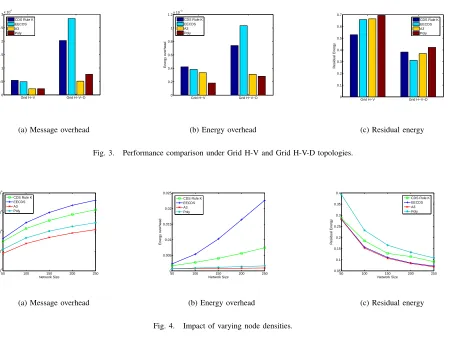
Simulation results are described in three subsections. First, we evaluate all the four protocols in two ideal grid en-vironments observed in controlled indoor deployments: the Grid V and the Grid V-D topologies. In the Grid H-V topology, nodes can communicate with their horizontal and vertical neighbors, while in the Grid H-V-D topology, nodes can communicate with their diagonal neighbors as well. Subsequently, we compare the protocols’ performances under varying node densities assuming that: (1) the nodes are randomly deployed, and (2) the protocols only construct the topology. We then discuss the performance of the protocols under a dynamic topology maintenance technique triggered by energy thresholds. In the next section, we model and compare the reliability of these protocols.

A. Grid Topology

1 2 3 4 5 6 7 8 9 10 11 12 13 14 15 16 17 18 19 20 21 22 23 24 25 26 27 28 29 30 31 32 33 34 35 36 37 38 39 40 41 42 43 44 45 46 47 48 49 50 51 52 53 54 55 56 57 58 59 60 61 62

6

Grid H−V Grid H−V−D 0

0.5 1 1.5 2 2.5 3x 10

4

Total Number of Messages

CDS Rule K EECDS A3 Poly

(a) Message overhead

Grid H−V Grid H−V−D 0

0.2 0.4 0.6 0.8 1 1.2x 10

−3

Energy overhead

CDS Rule K EECDS A3 Poly

(b) Energy overhead

Grid H−V Grid H−V−D 0

0.1 0.2 0.3 0.4 0.5 0.6 0.7

Residual Energy

CDS Rule K EECDS A3 Poly

(c) Residual energy

Fig. 3. Performance comparison under Grid H-V and Grid H-V-D topologies.

50 100 150 200 250 102

103

104

105

106

Network Size

Total Number of Messages (Log Scale)

CDS Rule K EECDS A3 Poly

(a) Message overhead

50 100 150 200 250 0

0.005 0.01 0.015 0.02 0.025

Network Size

Energy overhead

CDS Rule K EECDS A3 Poly

(b) Energy overhead

50 100 150 200 250 0.05

0.1 0.15 0.2 0.25 0.3 0.35 0.4

Network Size

Residual Energy

CDS Rule K EECDS A3 Poly

(c) Residual energy

Fig. 4. Impact of varying node densities.

B. Impact of Node Density

Figure 4 shows the message overhead, energy overhead and residual energy of all the four protocols. As the network size grows, the number of exchanged messages rises exponentially for all the four protocols. The increase in the node density results in a proportional increase in the node degree which ultimately leads to an increase in the number of messages exchanged. This trend is noticeable in the results shown in Figure 4(a). Number of exchanged messages for EECDS and CDS-Rule K is significantly higher than the Poly protocol. This is caused by the two-phase topology construction process utilized by EECDS and CDS-Rule K protocols.

In comparison, A3 generates fewer messages because it chooses the distant nodes using signal strength. This allows fewer nodes to become part of the CDS, thus leading to quick convergence of the protocol. On the other hand, the Poly protocol forms a polygon in which all the nodes send their IDs back to the parent node. This process incurs higher message overhead than the A3 protocol.

Energy overheads of EECDS and CDS-Rule K are signif-icantly higher than A3 and Poly, as shown in Figure 4(b). As can be intuitively argued, an increasing node density leads to higher energy consumption due to an increase in the number of received packets. However, Poly still has lower energy consumption due to its rebroadcast strategy for topology discovery. As mentioned earlier, Poly does not use

any messages explicitly sent to a parent node by its children. Instead, it overhears the broadcast at the parent node to get aware of its children. A3 protocol has less message overhead when compared with all the other three protocols. The energy overhead curve flattens for A3 and Poly protocols because both protocols do not use a two-phase strategy like EECDS and CDS-Rule K.

Figure 4(c) shows the residual energy of all the four pro-tocols. Usually, high energy overheads lead to lower residual energies. However, we observe that A3 which has low message and energy overheads, has significantly less residual energy. This is due to non-uniform distribution of communication overhead which drains the battery of fewer nodes resulting in lower residual energy levels among nodes in the network. On the other hand, EECDS and CDS-Rule K protocols have less residual energy due to high energy overhead. Poly provides better residual energy when compared with all the three protocols. This is because: 1) It forms the active node set in proportion to the network size, and 2) it uses a rebroadcast mechanism which inherently consumes battery of nodes at an equal rate.

C. Dynamic Topology Maintenance

2 3 4 5 6 7 8 9 10 11 12 13 14 15 16 17 18 19 20 21 22 23 24 25 26 27 28 29 30 31 32 33 34 35 36 37 38 39 40 41 42 43 44 45 46 47 48 49 50 51 52 53 54 55 56 57 58 59 60 61 62

50 100 150 200 250 104

105 106 107

Network Size

Total Number of Messages (Log Scale)

CDS Rule K EECDS A3 Poly

(a) Message overhead

50 100 150 200 250 0.1

0.2 0.3 0.4 0.5 0.6 0.7 0.8 0.9 1

Network Size

Energy overhead

CDS Rule K EECDS A3 Poly

(b) Energy overhead

50 100 150 200 250 0

0.05 0.1 0.15 0.2 0.25 0.3 0.35 0.4

Network Size

Residual Energy

CDS Rule K EECDS A3 Poly

(c) Residual energy

50 100 150 200 250 0

50 100 150 200 250

Network Size

Number of Unconnected Nodes

CDS Rule K EECDS A3 Poly

(d) Connectivity

Fig. 5. Performance comparison under dynamic topology maintenance.

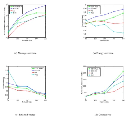
contribute to large number of exchanged messages as the network size is increased. This is shown in Figure 5(a). How-ever, the number of exchanged messages decreases slightly in case of CDS-Rule K protocol. This is due to less number of connected nodes as the node density is increased (see Fig. 5(d)). For A3 and Poly protocols, the number of exchanged messages increases exponentially due to higher number of connected nodes.

Similarly, consumed energy also increases linearly in case of EECDS and CDS-Rule K protocols (Figure 5(b)). However, EECDS allows uniform distribution of energy resources which results in better residual energy (Fig. 5(c)). On the other hand, CDS-Rule K uses a pruning process in which every node updates its two hop neighbors when it is not marked and the process gradually increases as the node density is changed. Therefore, CDS-Rule K has less residual energy as shown in Figure 5(c). A3 protocol shows consistent behavior in terms of energy overhead. However, it has less residual energy due to its three way message exchange and distant node selection

metric (see Fig. 5(c)). The energy overhead for Poly protocol decreases when the number of connected nodes gets lower. However, it has better residual energy when compared with all the three protocols as shown in Figure 5(c) for the reasons mentioned in the previous subsection.

Figure 5(d) shows the number of unconnected nodes un-der dynamic topology maintenance. In CDS-Rule K, nodes remained marked if there is at least one pair of unconnected neighbors. The energy depletion of the marked node leads to higher number of unconnected nodes as compared with the other three protocols. On the other hand, A3 has less number of unconnected nodes due to its node selection process based on signal strength metric. Performance of Poly in larger networks is better than EECDS and CDS-Rule K. However, it is alarming to note that the number of unconnected nodes increases as the network size gets bigger.

1 2 3 4 5 6 7 8 9 10 11 12 13 14 15 16 17 18 19 20 21 22 23 24 25 26 27 28 29 30 31 32 33 34 35 36 37 38 39 40 41 42 43 44 45 46 47 48 49 50 51 52 53 54 55 56 57 58 59 60 61 62

8

0.4 0.5 0.6 0.7 0.8 0.9 1.0 10−4

10−3 10−2 10−1 100

Link Probability

Network Reliability (Log Scale)

Actual Network Poly CDS

Fig. 6. Network Reliability

VI. NETWORKRELIABILITY

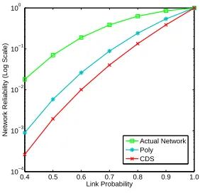
In graph theory, redundancy is defined as the expected number of functional spanning trees in a graph. Removal of an edge from a spanning tree partitions the graph. Therefore, every edge may be considered as a bridge in a spanning tree. The number of spanning trees measures the network performance under highly dynamic conditions, e.g. frequent link failures. Reliability, on the other hand, is the probability that there is at least one spanning tree or the probability that the sensor nodes can communicate with each other in case of random link failures. Hence, reliability is another critical parameter that measures the redundancy of the protocol [15]. We used linalg (Linear Algebra) package available in Maple [16] to analyze the performance of Poly protocol by assuming the network shown in Figure 1. We generated different random topologies of different size and averaged the reliability results. However, Poly provides similar results regardless of the un-derlying topology and network size due to polygenic nature of the protocol. Moreover, CDS protocols also provides similar behavior as they form a CDS tree.

LetA =(ai.j)n.n denote the adjacency matrix of graphG,

then

ai.j=

½

1 if verticesvi andvj are adjacent, 0 otherwise.

The degrees of the vertices are represented by a diagonal matrix. If D = (di.j)n.n denote the diagonal matrix of graph G, then

di.j=

½

deg(vi), fori=j, 0 i6=j.

We used the matrix tree theorem [15] to find the number of non-identical spanning trees for the network shown in Figure 1. According to the theorem, the spanning trees of graph G

is the value of any cofactor of the matrix, i.e. T = D−A. Therefore, the matrix T for the assumed network equals

T =

             

3 −1 0 0 0 −1 0 −1 0

−1 4 −1 −1 0 −1 0 0 0

0 −1 2 −1 0 0 0 0 0

0 −1 −1 4 −1 0 −1 0 0

0 0 0 −1 3 0 −1 −1 0

−1 −1 0 0 0 3 0 0 −1

0 0 0 −1 −1 0 2 0 0

−1 0 0 0 −1 0 0 2 0

0 0 0 0 0 −1 0 0 1

             

The cofactor of matrix T equals 108. Hence, there are 108 non-identical spanning trees which represent the total redundancy of the network. We are interested in measuring the probability that at least one of the spanning trees is working or the reliability that the network will be functional in events of random edge failures. To compute this, we must represent all spanning trees as a disjoint product as given below:

P(t1∨t2∨t3∨...∨t108) =P(t1) +P(t2t1) +P(t3t2t1)+

. . .+P(t108t107t106....t1),

wheretis a spanning tree in the network.

We computed the reliability for CDS (CDS RuleK, EECDS and A3) protocols and compared them with the proposed Poly protocol. The adjacency matrix for CDS-based protocols remains the same. Therefore, all the three protocols have the same reliability. Consequently, these existing protocols maintain a CDS tree in which every edge serves as a bridge edge. If we suppose that all edges have the same reliability

P1=P2=....=Pn =P then the reliability of the network shown in Figure 1 is given by: 108p8_−315p9_{+ 348p}10₋

172p11_{+ 32p}12_.

Figure 6 compares the reliability of poly protocol with CDS based protocols. The decrease in the link probability causes a proportional decrease in the network reliability. However, the Poly protocol provides better network reliability as the link probability is decreased. Existing CDS-based protocols have considerably lower network reliability because each edge (link) in these topologies serves as a bridge edge, and therefore does not provide any redundancy in the network.

VII. CONCLUSIONS

In this paper, we proposed a topology control protocol – Poly – which forms a CDS by finding polygons present in a WSN. We performed simulations to compare the performance of Poly with other prominent topology construction protocols– CDS-Rule K, A3 and EECDS–over a large operational spec-trum. Simulation results demonstrated that Poly has low message overhead and energy consumption, and can provide higher network reliability. The Poly protocol also works well with dynamic topology maintenance techniques.

REFERENCES

2 3 4 5 6 7 8 9 10 11 12 13 14 15 16 17 18 19 20 21 22 23 24 25 26 27 28 29 30 31 32 33 34 35 36 37 38 39 40 41 42 43 44 45 46 47 48 49 50 51 52 53 54 55 56 57 58 59 60 61 62

[2] P. J. Wan, K. M. Alzoubi, and O. Frieder, “Distributed Construction of Connected Dominating Sets in Wireless Ad Hoc Networks,”IEEE INFOCOM, 2002.

[3] H. K. Qureshi, S. Rizvi, M. Saleem, S. A. Khayam, V. Rakocevic, and M. Rajarajan, “An Energy Efficient Clique-based CDS Discovery Protocol for Wireless Sensor Networks,” In proceedings of 44th Annual conference on Information Sciences and Systems(CISS), March, 2010. [4] M. Gerla and J. T. Tsai, “Multicluster mobile multimedia radio network,“

ACM Wireless Networks, vol. 1(3), pp. 255-265, 1995.

[5] P. M. Wightman and M. A. Labrador, “A3: A Topology Construction Algorithm for Wireless Sensor Network,” Proc.IEEE Globecom, 2008. [6] Z. Yuanyuan, X. Jia, and H. Yanxiang, “Energy efficient distributed connected dominating sets construction in wireless sensor networks,” In Proceedings of theACM International Conference on Communications and Mobile Computing, pp. 797-802, 2006.

[7] J. Wu, M. Cardei, F. Dai, and S. Yang, “Extended dominating set and its applications in ad hoc networks using cooperative communication,” IEEE Trans. on Parallel and Distributed Systems, vol. 17(8), pp. 851-864, 2006.

[8] F. Wang, M. T. Thai, D. Z. Du, ”On the construction of 2-connected Virtual Backbone in Wireless Network”, Accpeted by IEEE Transactions on Wireless Communications, 2007.

[9] Y. Wu, F. Wang, M. T. Thai and Y. Li, ”Constructing k-Connected m-Dominating Sets in Wireless Sensor Networks”, Military Communica-tions Conference, Orlando, FL, October 29-31, 2007.

[10] G. Xing, T. Wang, W. Jia and M. Li, “Rendezvous Design Algorithms for Wireless Sensor Networks with a Mobile Base Station,”In Proceedings of the9th ACM International Symposium on Mobile Ad Hoc Networking and Computing (MobiHoc), May, 2008.

[11] R. Ramanathan and R. Rosales-Hain, “Topology control of Multihop Wireless Networks Using Transmit Power adjustment,”IEEE Infocom, pp. 404-413, 2000.

[12] V. Rodoplu and T.H.Meng, “Minimum Energy Mobile Wireless Net-works,”IEEE J. Selected Areas in Comm., vol.17, n.8, pp.1333-1344, Aug. 1999.

[13] D. J. Baker and A. Ephremides, “The architectural organization of a mobile radio network via a distributed algorithm,” IEEE Transactions on Communications, pp. 1694-1701, 1981.

[14] P. M. Wightman and M. A. Labrador, “Atarraya: A Simulation Tool to Teach and Research Topology Control Algorithms for Wireless Sensor Networks,” Create-Net 2nd International Conference on Simulation Tools and Techniques, SIMUTools, 2009.

[15] P.G. Ralph, “Discrete and Combinatorial Mathematics: An applied Introduction,” 3rd edition, Addison-Wesley, Reading, MA, 1994. [16] Maple homepage, http://www.maplesoft.com.