Upper limits on gravitational wave bursts in LIGO’s second science run
B. Abbott,12R. Abbott,15R. Adhikari,12A. Ageev,20,27J. Agresti,12B. Allen,39J. Allen,13R. Amin,16S. B. Anderson,12 W. G. Anderson,29M. Araya,12H. Armandula,12M. Ashley,28F. Asiri,12,aP. Aufmuth,31C. Aulbert,1S. Babak,7 R. Balasubramanian,7S. Ballmer,13B. C. Barish,12C. Barker,14D. Barker,14M. Barnes,12,bB. Barr,35M. A. Barton,12
K. Bayer,13R. Beausoleil,26,cK. Belczynski,23R. Bennett,35,dS. J. Berukoff,1,eJ. Betzwieser,13B. Bhawal,12 I. A. Bilenko,20G. Billingsley,12E. Black,12K. Blackburn,12L. Blackburn,13B. Bland,14B. Bochner,13,fL. Bogue,15 R. Bork,12S. Bose,41P. R. Brady,39V. B. Braginsky,20J. E. Brau,37D. A. Brown,12A. Bullington,26A. Bunkowski,2,31
A. Buonanno,6,gR. Burgess,13D. Busby,12W. E. Butler,38R. L. Byer,26L. Cadonati,13G. Cagnoli,35J. B. Camp,21 J. Cannizzo,21K. Cannon,39C. A. Cantley,35L. Cardenas,12K. Carter,15M. M. Casey,35J. Castiglione,34A. Chandler,12 J. Chapsky,12,bP. Charlton,12,hS. Chatterji,12S. Chelkowski,2,31Y. Chen,1V. Chickarmane,16,iD. Chin,36N. Christensen,8
D. Churches,7T. Cokelaer,7C. Colacino,33R. Coldwell,34M. Coles,15,jD. Cook,14T. Corbitt,13D. Coyne,12 J. D. E. Creighton,39T. D. Creighton,12D. R. M. Crooks,35P. Csatorday,13B. J. Cusack,3C. Cutler,1J. Dalrymple,27
E. D’Ambrosio,12K. Danzmann,2,31G. Davies,7E. Daw,16,kD. DeBra,26T. Delker,34,lV. Dergachev,36S. Desai,28 R. DeSalvo,12S. Dhurandhar,11A. Di Credico,27M. Dı´az,29H. Ding,12R. W. P. Drever,4R. J. Dupuis,12J. A. Edlund,12,b P. Ehrens,12E. J. Elliffe,35T. Etzel,12M. Evans,12T. Evans,15S. Fairhurst,39C. Fallnich,31D. Farnham,12M. M. Fejer,26 T. Findley,25M. Fine,12L. S. Finn,28K. Y. Franzen,34A. Freise,2,mR. Frey,37P. Fritschel,13V. V. Frolov,15M. Fyffe,15
K. S. Ganezer,5J. Garofoli,14J. A. Giaime,16A. Gillespie,12,nK. Goda,13L. Goggin,12G. Gonza´lez,16S. Goßler,31 P. Grandcle´ment,23,oA. Grant,35C. Gray,14A. M. Gretarsson,15,pD. Grimmett,12H. Grote,2S. Grunewald,1M. Guenther,14 E. Gustafson,26,qR. Gustafson,36W. O. Hamilton,16M. Hammond,15J. Hanson,15C. Hardham,26J. Harms,19G. Harry,13
A. Hartunian,12J. Heefner,12Y. Hefetz,13G. Heinzel,2I. S. Heng,31M. Hennessy,26N. Hepler,28A. Heptonstall,35 M. Heurs,31M. Hewitson,2S. Hild,2N. Hindman,14P. Hoang,12J. Hough,35M. Hrynevych,12,rW. Hua,26M. Ito,37Y. Itoh,1
A. Ivanov,12O. Jennrich,35,sB. Johnson,14W. W. Johnson,16W. R. Johnston,29D. I. Jones,28G. Jones,7L. Jones,12 D. Jungwirth,12,tV. Kalogera,23E. Katsavounidis,13K. Kawabe,14S. Kawamura,22W. Kells,12J. Kern,15,uA. Khan,15 S. Killbourn,35C. J. Killow,35C. Kim,23C. King,12P. King,12S. Klimenko,34S. Koranda,39K. Ko¨tter,31J. Kovalik,15,b D. Kozak,12B. Krishnan,1M. Landry,14J. Langdale,15B. Lantz,26R. Lawrence,13A. Lazzarini,12M. Lei,12I. Leonor,37 K. Libbrecht,12A. Libson,8P. Lindquist,12S. Liu,12J. Logan,12,uM. Lormand,15M. Lubinski,14H. Lu¨ck,2,31M. Luna,32
T. T. Lyons,12,vB. Machenschalk,1M. MacInnis,13M. Mageswaran,12K. Mailand,12W. Majid,12,bM. Malec,2,31 V. Mandic,12F. Mann,12A. Marin,13,wS. Ma´rka,9E. Maros,12J. Mason,12,xK. Mason,13O. Matherny,14L. Matone,9
N. Mavalvala,13R. McCarthy,14D. E. McClelland,3M. McHugh,18A. Melissinos,38G. Mendell,14R. A. Mercer,33 S. Meshkov,12E. Messaritaki,39C. Messenger,33E. Mikhailov,13S. Mitra,11V. P. Mitrofanov,20G. Mitselmakher,34 R. Mittleman,13O. Miyakawa,12S. Miyoki,12,yS. Mohanty,29G. Moreno,14K. Mossavi,2G. Mueller,34S. Mukherjee,29
P. Murray,35E. Myers,40J. Myers,14S. Nagano,2T. Nash,12R. Nayak,11G. Newton,35F. Nocera,12J. S. Noel,41 P. Nutzman,23T. Olson,24B. O’Reilly,15D. J. Ottaway,13A. Ottewill,39,zD. Ouimette,12,tH. Overmier,15B. J. Owen,28
Y. Pan,6M. A. Papa,1V. Parameshwaraiah,14P. Ajith,2C. Parameswariah,15M. Pedraza,12S. Penn,10M. Pitkin,35 M. Plissi,35R. Prix,1V. Quetschke,34F. Raab,1H. Radkins,14R. Rahkola,37M. Rakhmanov,34S. R. Rao,12K. Rawlins,13 S. Ray-Majumder,39V. Re,33D. Redding,12,bM. W. Regehr,12,bT. Regimbau,7S. Reid,35K. T. Reilly,12K. Reithmaier,12 D. H. Reitze,34S. Richman,13,{R. Riesen,15K. Riles,36B. Rivera,14A. Rizzi,15,|D. I. Robertson,35N. A. Robertson,26,35 C. Robinson,7L. Robison,12S. Roddy,15A. Rodriguez,16J. Rollins,9J. D. Romano,7J. Romie,12H. Rong,34,nD. Rose,12 E. Rotthoff,28S. Rowan,35A. Ru¨diger,2L. Ruet,13P. Russell,12K. Ryan,14I. Salzman,12V. Sandberg,14G. H. Sanders,12,} V. Sannibale,12P. Sarin,13B. Sathyaprakash,7P. R. Saulson,27R. Savage,14A. Sazonov,34R. Schilling,2K. Schlaufman,28 V. Schmidt,12,~R. Schnabel,19R. Schofield,37B. F. Schutz,1,7P. Schwinberg,14S. M. Scott,3S. E. Seader,41A. C. Searle,3 B. Sears,12S. Seel,12F. Seifert,19D. Sellers,15A. S. Sengupta,11C. A. Shapiro,28,P. Shawhan,12D. H. Shoemaker,13 Q. Z. Shu,34,A. Sibley,15X. Siemens,39L. Sievers,12,bD. Sigg,14A. M. Sintes,1,32J. R. Smith,2M. Smith,13M. R. Smith,12
P. H. Sneddon,35R. Spero,12,bO. Spjeld,15G. Stapfer,15D. Steussy,8K. A. Strain,35D. Strom,37A. Stuver,28 T. Summerscales,28M. C. Sumner,12M. Sung,16P. J. Sutton,12J. Sylvestre,12, A. Takamori,12, D. B. Tanner,34H. Tariq,12
P. A. Willems,12P. R. Williams,1,R. Williams,4B. Willke,2,31A. Wilson,12B. J. Winjum,28,eW. Winkler,2S. Wise,34 A. G. Wiseman,39G. Woan,35D. Woods,39R. Wooley,15J. Worden,14W. Wu,34I. Yakushin,15H. Yamamoto,12
S. Yoshida,25K. D. Zaleski,28M. Zanolin,13I. Zawischa,31,L. Zhang,12R. Zhu,1N. Zotov,17 M. Zucker,15and J. Zweizig12
(The LIGO Scientific Collaboration)
1Albert-Einstein-Institut, Max-Planck-Institut fu¨r Gravitationsphysik, D-14476 Golm, Germany 2Albert-Einstein-Institut, Max-Planck-Institut fu¨r Gravitationsphysik, D-30167 Hannover, Germany
3Australian National University, Canberra, 0200, Australia 4California Institute of Technology, Pasadena, California 91125, USA 5
California State University Dominguez Hills, Carson, California 90747, USA
6Caltech-CaRT, Pasadena, California 91125, USA 7Cardiff University, Cardiff, CF2 3YB, United Kingdom
8Carleton College, Northfield, Minnesota 55057, USA 9Columbia University, New York, New York 10027, USA 10Hobart and William Smith Colleges, Geneva, New York 14456, USA 11Inter-University Centre for Astronomy and Astrophysics, Pune 411007, India 12LIGO—California Institute of Technology, Pasadena, California 91125, USA 13LIGO—Massachusetts Institute of Technology, Cambridge, Massachusetts 02139, USA
14LIGO Hanford Observatory, Richland, Washington 99352, USA 15LIGO Livingston Observatory, Livingston, Louisiana 70754, USA
16Louisiana State University, Baton Rouge, Louisiana 70803, USA 17Louisiana Tech University, Ruston, Louisiana 71272, USA
18Loyola University, New Orleans, Louisiana 70118, USA 19Max Planck Institut fu¨r Quantenoptik, D-85748, Garching, Germany
20Moscow State University, Moscow, 119992, Russia
21NASA/Goddard Space Flight Center, Greenbelt, Maryland 20771, USA 22National Astronomical Observatory of Japan, Tokyo 181-8588, Japan
23Northwestern University, Evanston, Illinois 60208, USA 24Salish Kootenai College, Pablo, Montana 59855, USA 25Southeastern Louisiana University, Hammond, Louisiana 70402, USA
26Stanford University, Stanford, California 94305, USA 27Syracuse University, Syracuse, New York 13244, USA
28The Pennsylvania State University, University Park, Pennsylvania 16802, USA
29The University of Texas at Brownsville and Texas Southmost College, Brownsville, Texas 78520, USA 30Trinity University, San Antonio, Texas 78212, USA
31Universita¨t Hannover, D-30167 Hannover, Germany 32Universitat de les Illes Balears, E-07122 Palma de Mallorca, Spain
33University of Birmingham, Birmingham, B15 2TT, United Kingdom 34University of Florida, Gainesville, Florida 32611, USA 35University of Glasgow, Glasgow, G12 8QQ, United Kingdom
36University of Michigan, Ann Arbor, Michigan 48109, USA 37University of Oregon, Eugene, Oregon 97403, USA 38University of Rochester, Rochester, New York 14627, USA 39University of Wisconsin-Milwaukee, Milwaukee, Wisconsin 53201, USA
40Vassar College, Poughkeepsie, New York 12604, USA 41Washington State University, Pullman, Washington 99164, USA
(Received 7 June 2005; published 8 September 2005)
We perform a search for gravitational wave bursts using data from the second science run of the LIGO detectors, using a method based on a wavelet time-frequency decomposition. This search is sensitive to bursts of duration much less than a second and with frequency content in the 100 –1100 Hz range. It features significant improvements in the instrument sensitivity and in the analysis pipeline with respect to the burst search previously reported by LIGO. Improvements in the search method allow exploring weaker signals, relative to the detector noise floor, while maintaining a low false alarm rate,O0:1Hz. The sensitivity in terms of theroot-sum-square (rss) strain amplitude lies in the range of hrss1020
1019 Hz1=2. No gravitational wave signals were detected in 9.98 days of analyzed data. We interpret the
detection efficiency for selected waveform morphologies in order to yield rate versus strength exclusion curves as well as to establish order-of-magnitude distance sensitivity to certain modeled astrophysical sources. Both the rate upper limit and its applicability to signal strengths improve our previously reported limits and reflect the most sensitive broad-band search for untriggered and unmodeled gravitational wave bursts to date.
DOI:10.1103/PhysRevD.72.062001 PACS numbers: 04.80.Nn, 07.05.Kf, 95.30.Sf, 95.85.Sz
I. INTRODUCTION
The Laser Interferometer Gravitational wave Ob-servatory (LIGO) is a network of interferometric detectors aiming to make direct observations of gravitational waves. Construction of the LIGO detectors is essentially com-plete, and much progress has been made in commissioning them to (a) bring the three interferometers to their final optical configuration, (b) reduce the interferometers’ noise floors and improve the stationarity of the noise, and (c) pave the way toward long-term science observations. Interleaved with commissioning, four ‘‘science runs’’ have been carried out to collect data under stable operating conditions for astrophysical gravitational wave searches, albeit at reduced sensitivity and observation time relative to the LIGO design goals. The first science run, called S1, took place in the summer of 2002 over a period of 17 days. S1 represented a major milestone as the longest and most sensitive operation of broad-band interferometersin coin-cidenceup to that time. Using the S1 data from the LIGO and GEO600 interferometers [1], astrophysical searches
for four general categories of gravitational wave source types —binary inspiral [2], burst[3], stochastic [4], and continuous wave [5]— were pursued by the LIGO Scientific Collaboration (LSC). These searches established general methodologies to be followed and improved upon for the analysis of data from future runs. In 2003 two additional science runs of the LIGO instruments collected data of improved sensitivity with respect to S1, but still less sensitive than the instruments’ design goal. The second science run (S2) collected data in early 2003 and the third science run (S3) at the end of the same year. Several searches have been completed or are underway using data from the S2 and S3 runs [6 –13]. A fourth science run, S4, took place at the beginning of 2005.
In this paper we report the results of a search for gravi-tational wave bursts using the LIGO S2 data. The astro-physical motivation for burst events is strong; it embraces catastrophic phenomena in the universe with or without clear signatures in the electromagnetic spectrum, such as supernova explosions [14 –16], the merging of compact binary stars as they form a single black hole [17–19], and the astrophysical engines that power the gamma ray bursts [20]. Perturbed or accreting black holes, neutron star os-cillation modes and instabilities as well as cosmic string cusps and kinks [21] are also potential burst sources. The expected rate, strength and waveform morphology for such events is not generally known. For this reason, our assump-tions about the expected signals are minimal. The experi-mental signatures on which this search focused can be described as burst signals of short duration ( 1 s) [22] and with enough signal strength in the LIGO sensitive band (100 –1100 Hz) to be detected in coincidence in all three LIGO instruments. The triple-coincidence requirement is used to reduce the false alarm rate (background) to much less than one event over the course of the run, so that even a
aCurrently at Stanford Linear Accelerator Center bCurrently at Jet Propulsion Laboratory
cPermanent Address: HP Laboratories dCurrently at Rutherford Appleton Laboratory eCurrently at University of California, Los Angeles fCurrently at Hofstra University
gPermanent Address: GReCO, Institut d’Astrophysique de Paris (CNRS)
hCurrently at Charles Sturt University, Australia iCurrently at Keck Graduate Institute
jCurrently at National Science Foundation kCurrently at University of Sheffield
lCurrently at Ball Aerospace Corporation mCurrently at European Gravitational Observatory
nCurrently at Intel Corp.
oCurrently at University of Tours, France
pCurrently at Embry-Riddle Aeronautical University qCurrently at Lightconnect Inc.
rCurrently at W. M. Keck Observatory
sCurrently at ESA Science and Technology Center tCurrently at Raytheon Corporation
uCurrently at New Mexico Institute of Mining and Technology/Magdalena Ridge Observatory Interferometer
vCurrently at Mission Research Corporation w
Currently at Harvard University
yPermanent Address: University of Tokyo, Institute for Cosmic Ray Research
zPermanent Address: University College Dublin
aaCurrently at Research Electro-Optics Inc.
abCurrently at Institute of Advanced Physics, Baton Rouge, LA acCurrently at Thirty Meter Telescope Project at Caltech adCurrently at European Commission, DG Research, Brussels, Belgium
aeCurrently at University of Chicago afCurrently at LightBit Corporation agPermanent Address: IBM Canada Ltd. ahCurrently at The University of Tokyo
ai
Currently at University of Delaware
ajPermanent Address: Jet Propulsion Laboratory akCurrently at Shanghai Astronomical Observatory
single event candidate would have high statistical significance.
The general methodology in pursuing this search follows the one we presented in the analysis of the S1 data [3] with some significant improvements. In the S1 analysis the ringing of the prefilters limited our ability to perform tight time-coincidence between the triggers coming from the three LIGO instruments. This is addressed by the use of a new search method that does not require strong prefilter-ing. This new method also provides improved event pa-rameter estimation, including timing resolution. Finally, a waveform consistency test is introduced for events that pass the time and frequency coincidence requirements in the three LIGO detectors.
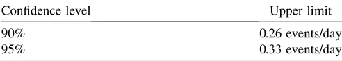
This search examines 9.98 days of live time and yields one candidate event in coincidence among the three LIGO detectors during S2. Subsequent examination of this event reveals an acoustic origin for the signal in the two Hanford detectors, easily eliminated using a ‘‘veto’’ based on acous-tic power in a microphone. Taking this into account, we set an upper limit on the rate of burst events detectable by our detectors at the level of 0.26 per day at an estimated 90% confidence level. We have usedad hocwaveforms (sine-Gaussians and (sine-Gaussians) to establish the sensitivity of the S2 search pipeline and to interpret our upper limit as an excluded region in the space of signal rate versus strength. The burst search sensitivity in terms of theroot-sum-square (rss) strain amplitude incident on Earth lies in the range hrss10201019 Hz1=2. Both the upper limit (rate) and its applicability to signal strengths (sensitivity) reflect significant improvements with respect to our S1 result [3]. In addition, we evaluate the sensitivity of the search to astrophysically motivated waveforms derived from models of stellar core collapse [14 –16] and from the merger of binary black holes [17,18].
In the following sections we describe the LIGO instru-ments and the S2 run in more detail (Sec. II) as well as an overview of the search pipeline (Sec. III). The procedure for selecting the data that we analyze is described in Sec. IV. We then present the search algorithm and the waveform consistency test used in the event selection (Sec. V) and discuss the role of vetoes in this search (Sec. VI). Section VII describes the final event analysis and the assignment of an upper limit on the rate of detect-able bursts. The efficiency of the search for various target waveforms is presented in Sec. VIII. Our final results and discussion are presented in Secs. IX and X.
II. THE SECOND LIGO SCIENCE RUN
LIGO comprises three interferometers at two sites: an interferometer with 4 km long arms at the LIGO Livingston Observatory in Louisiana (denoted L1) and interferometers with 4 km and 2 km long arms in a com-mon vacuum system at the LIGO Hanford Observatory in Washington (denoted H1 and H2). All are Michelson
in-terferometers with power recycling and resonant cavities in the two arms to increase the storage time (and conse-quently the phase shift) for the light returning to the beam splitter due to motions of the end mirrors [23]. The mirrors are suspended as pendulums from vibration-isolated platforms to protect them from external noise sources. A detailed description of the LIGO detectors as they were configured for the S1 run may be found in Ref. [1].
A. Improvements to the LIGO detectors for S2
The LIGO interferometers [1,24] are still undergoing commissioning and have not yet reached their final oper-ating configuration and sensitivity. Between S1 and S2 a number of changes were made which resulted in improved sensitivity as well as overall instrument stability and sta-tionarity. The most important of these are summarized below.
The mirrors’ analog suspension controller electronics on the H2 and L1 interferometers were replaced with digital controllers of the type installed on H1 before the S1 run. The addition of a separate DC bias supply for alignment relieved the range requirement of the suspensions’ coil drivers. This, combined with flexibility of a digital system capable of coordinated switching of analog and digital filters, enabled the new coil drivers to operate with much lower electronics output noise. In particular, the system had two separate modes of operation: acquisition mode with larger range and noise, and run mode with reduced range and noise. A matched pair of filters was used to minimize noise in the coil current due to the discrete steps in the digital to analog converter (DAC) at the output of the digital suspension controller: a digital filter before the DAC boosted the high-frequency component relative to the low frequency component, and an analog filter after the DAC restored their relative amplitudes. Better filtering, better diagonalization of the drive to the coils to eliminate length-to-angle couplings and more flexible control/se-quencing features also contributed to an overall perform-ance improvement.
The noise from the optical lever servos that damp the angular excitations of the interferometer optics was re-duced. The mechanical support elements for the optical transmitter and receiver were stiffened to reduce low fre-quency vibrational excitations. Taking advantage of the low frequency improvements, input noise to the servo due to the discrete steps in the analog to digital converter (ADC) was reduced by a filter pair surrounding the ADC: an analog filter to whiten the data going into the ADC and a digital filter to restore it to its full dynamic range.
for the main interferometer (plus 4 degrees of freedom for the mode cleaner) controlled by their WFS. For S2, the H1 interferometer had 8 out of 16 alignment degrees of free-dom for the main interferometer under WFS control. As a result, it maintained a much more uniform operating point over the run than the other two interferometers, which continued to have only 2 degrees of freedom under WFS control.
The high frequency sensitivity was increased by operat-ing the interferometers with higher effective power. Two main factors enabled this power increase. Improved align-ment techniques and better alignalign-ment stability (due to the optical lever and wavefront sensor improvements de-scribed above) reduced the amount of spurious light at the antisymmetric port, which would have saturated the photodiode if the laser power had been increased in S1. Also, a new servo system to cancel the out-of-phase (non-signal) photocurrent in the antisymmetric photodiode was added. This amplitude of the out-of-phase photocurrent is nominally zero for a perfectly aligned and matched inter-ferometer, but various imperfections in the interferometer can lead to large low frequency signals. The new servo prevents these signals from causing saturations in the photodiode and its RF preamplifier. During S2, the inter-ferometers operated with about 1.5 W incident on the mode cleaner and about 40 W incident on the beam splitter.
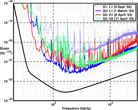
These changes led to a significant improvement in de-tector sensitivity. Figure 1 shows typical spectra achieved by the LIGO interferometers during the S2 run compared with LIGO’s S1 and design sensitivity. The differences among the three LIGO S2 spectra reflect differences in the operating parameters and hardware implementations of
the three instruments, which were in various stages of reaching the final design configuration.
B. Data from the S2 run
The data analyzed in this paper were taken during LIGO’s second science run (S2), which spanned 59 days from February 14 to April 14, 2003. During this time, operators and scientific monitors attempted to maintain continuous low noise operation of the LIGO instruments. The duty cycles for the individual interferometers, defined as the fraction of the total run time when the interferometer was locked (i.e., all interferometer control servos operating in their linear regime) and in its low noise configuration, were 74% for H1, 58% for H2, and 38% for L1; the triple-coincidence duty cycle (i.e., the time during which all three interferometers were simultaneously in lock and in low noise configuration) was 22%. The longest continuous locked stretch for any interferometer during S2 was 66 hours for H1. The main sources of lost time were high microseismic motion at both sites due to storms, and anthropogenic noise in the vicinity of the Livingston Observatory.
Improved monitoring and automated alarms instituted after S1 gave the operators and scientific monitors better warnings of out-of-nominal operating conditions for the interferometers. As a result, the fraction of time lost to high noise or to missing calibration lines (both major sources of unanalyzable data during the S1 run) was greatly reduced. Thus, even though the S2 run was less than a factor of 4 longer than the S1 run and the duty cycle for triple inter-ferometer coincidence was in fact marginally lower (23% for S1 vs 22% for S2), the total amount of analyzable triple-coincidence data was 305 hours compared to 34 hours for S1.
The signature of a gravitational wave is a differential change in the lengths of the two interferometer arms relative to the nominal lengths established by the control system, st Lxt Lyt=L, where Lis the av-erage length of thexandyarms. As in S1, this time series was derived from the error signal of the feedback loop used to differentially control the lengths of the interferometer arms in order to keep the optical cavities on resonance. To calibrate the error signal, the effect of the feedback loop gain was measured and divided out. Although more stable than during S1, the response functions varied over the course of the S2 run due to drifts in the alignment of the optical elements. These were tracked by injecting fixed-amplitude sinusoidal signals (calibration lines) into the differential arm control loop, and monitoring the ampli-tudes of these signals at the measurement (error) point [25].
The S2 run also involved coincident running with the TAMA interferometer [26]. TAMA achieved a duty cycle of 82% and had a sensitivity comparable to LIGO’s above
1 kHz, but had poorer sensitivity at lower frequencies
102 103
10−23 10−22 10−21 10−20 10−19 10−18
Frequency (Hertz) Strain
(Hz−1/2)
S1: L1 (9 Sept ’02) S2: L1 (1 March ’03) S2: H1 (8 April ’03) S2: H2 (11 April ’03)
FIG. 1 (color online). Typical LIGO strain sensitivities in units ofHz1=2 during the second science run (S2), compared to the
most sensitive detector (L1) during the S1 science run. The solid line denotes the design goal for the 4 km instruments.
[image:5.612.56.298.469.662.2]where the LIGO detectors had their best sensitivity. In addition, the location and orientation of the TAMA detec-tor differs substantially from the LIGO detecdetec-tors, which further reduced the chance of a coincident detection at low frequencies. For these reasons, the joint analysis of LIGO and TAMA data focused on gravitational wave frequencies from 700 – 2000 Hz and will be described in a separate paper [10]. In this paper, we report the result of a LIGO-only search for signals in the range 100 –1100 Hz. The overlap between these two searches (700 –1100 Hz) serves to ensure that possible sources with frequency content spanning the two searches will not be missed. The GEO600 interferometer [27], which collected data simul-taneously with LIGO during the S1 run, was undergoing commissioning at the time of the S2 run.
III. SEARCH PIPELINE OVERVIEW
The overall burst search pipeline used in the S2 analysis follows the one we introduced in our S1 search [3]. First, data selection criteria are applied in order to define periods when the instruments are well behaved and the recorded data can be used for science searches (Sec. IV).
A wavelet-based algorithm called WaveBurst [28,29] (Sec. VA) is then used to identify candidate burst events. Rather than operating on the data from a single interfer-ometer, WaveBurst analyzes simultaneously the time series coming from a pair of interferometers and incorporates strength thresholding as well as time and frequency coin-cidence to identify transients with consistent features in the two data streams. To reduce the false alarm rate, we further require that candidate gravitational wave events occur effectively simultaneously in all three LIGO detectors (Sec. V B). Besides requiring compatible WaveBurst event parameters, this involves a waveform consistency test, the rstatistic [30] (Sec. V C), which is based on forming the normalized linear correlation of the raw time series coming from the LIGO instruments. This test takes advantage of the fact that the arms of the interferometers at the two LIGO sites are nearly coaligned, and therefore a gravita-tional wave generally will produce correlated time series. The use of WaveBurst and the r statistic are the major changes in the S2 pipeline with respect to the pipeline used for S1 [3].
When candidate burst events are identified, they can be checked against veto conditions based on the many auxil-iary readback channels of the servo control systems and physical environment monitoring channels that are re-corded in the LIGO data stream (Sec. VI).
The background in this search is measured by artificially shifting in time the raw time series of one of the LIGO instruments, L1, and repeating the analysis as for the unshifted data. The time-shifted case will often be referred to as ‘‘time-lag’’ data and the unshifted case as ‘‘zero-lag’’ data. We will describe the background estimation in more detail in Sec. VII.
We have relied on hardware and software signal ‘‘in-jections’’ in order to establish the efficiency of the pipeline. Simulated signals with various morphologies [31] were added to the digitized raw data time series at the beginning of our analysis pipeline and were used to establish the fraction of detected events as a function of their strength (Sec. VIII). The same analysis pipeline was used to analyze raw (zero-lag), time-lag, and injection data samples.
We maintain a detailed list with a number of checks to perform for any zero-lag event(s) surviving the analysis pipeline to evaluate whether they could plausibly be gravi-tational wave bursts. This ‘‘detection checklist’’ is updated as we learn more about the instruments and refine our methodology. A major aspect is the examination of envi-ronmental and auxiliary interferometric channels in order to identify terrestrial disturbances that might produce a candidate event through some coupling mechanism. Any remaining events are compared with the background and the experiment’s live time in order to establish a detection or an upper limit on the rate of burst events.
IV. DATA SELECTION
The selection of data to be analyzed was a key first step in this search. We expect a gravitational wave to appear in all three LIGO instruments, although in some cases it may be at or below the level of the noise. For this search, we requirea signal above the noise baseline in all three instru-ments in order to suppress the rate of noise fluctuations that may fake astrophysical burst events. In the case of a genuine astrophysical event this requirement will not only increase our detection confidence but it will also allow us to extract in the best possible way the signal and source parameters. Therefore, for this search we have confined ourselves to periods of time when all three LIGO interfer-ometers were simultaneously locked in low noise mode with nominal operating parameters (servo loop gains, filter settings, etc.), marked by a manually set bit (‘‘science mode’’) in the data stream. This produced a total of 318 hours of potential data for analysis. This total was reduced by the following data selection cuts:
(i) A minimum duration of 300 seconds was required for a triple-coincidence segment to be analyzed for this search. This cut eliminated 0.9% of the initial data set.
(ii) Post-run re-examination of the interferometer con-figuration and status channels included in the data stream identified a small amount of time when the interferometer configuration deviated from nomi-nal. In addition we identified short periods of time when the timing system for the data acquisition had lost synchronization. These cuts reduced the data set by 0.2%.
caused bursts of excess noise due to nonlinear up-conversion. These periods of time were identified and eliminated, reducing the data set by 0.3%. (iv) There were occasional periods of time when the
calibration lines either were absent or were signifi-cantly weaker than normal. Eliminating these peri-ods reduced the data set by approximately 2%. (v) The H1 interferometer had a known problem with a
marginally stable servo loop, which occasionally led to higher than normal noise in the error signal for the differential arm length (the channel used in this search for gravitational waves). A data cut was imposed to eliminate periods of time when the root-mean-square (rms) noise in the 200 – 400 Hz band of this channel exceeded a threshold value for 5 consecutive minutes. The requirement for 5 con-secutive minutes was imposed to prevent a short burst of gravitational waves (the object of this search) from triggering this cut. This cut reduced the data set by 0.4%.
These data quality cuts eliminated a total of 13 hours from the original 318 hours of triple-coincidence data, leaving a ‘‘live-time’’ of 305 hours. The fraction of data surviving these quality cuts (96%) is a significant improve-ment over the experience in S1 when only 37% of the data passed all the quality cuts.
The trigger generation software used in this search (to be described in the next section) processed data in fixed 2-minute time intervals, requiring good data quality for the entire interval. This constraint, along with other constraints imposed by other trigger generation methods which were initially used to define a common data set, led to a net loss of 41 hours, leaving 264 hours of triple-coincidence data actually searched.
The search for bursts in the LIGO S2 data used roughly 10% of the triple-coincidence data set in order to tune the pipeline (as described below) and establish event selection criteria. This data set was chosen uniformly across the acquisition time and constituted the so-called ‘‘play-ground’’ for the search. The rate bound calculated in Sec. VII reflects only the remaining90%of the data, in order to avoid bias from the tuning procedures.
V. METHODS FOR EVENT TRIGGER SELECTION
An accurate knowledge of gravitational wave burst waveforms would allow the use ofmatched filtering[32] along the lines of the search for binary inspirals [2,8]. However, many different astrophysical systems may give rise to gravitational wave bursts, and the physics of these systems is often very complicated. Even when numerical relativistic calculations have been carried out, as in the case of core collapse supernovae, they generally yield roughly representative waveforms rather than exact pre-dictions. Therefore, our present searches for gravitational
wave bursts use general algorithms which are sensitive to a wide range of potential signals.
The first LIGO burst search [3] used two Event Trigger Generator (ETG) algorithms: a time-domain method de-signed to detect a large ‘‘slope’’ (time derivative) in the data stream after suitable filtering [33,34], and a method called TFCLUSTERS [35] which is based on identifying clusters of excess power in time-frequency spectrograms. Several other burst search methods have been developed by members of the LIGO Scientific Collaboration. For this paper, we have chosen to focus on a single ETG called WaveBurst which identifies clusters of excess power once the signal is decomposed in the wavelet domain, as de-scribed below. Other methods which were applied to the S2 data include TFCLUSTERS; the excess power statistic of Anderson et al. [36]; and the ‘‘Block-Normal’’ time-domain change-point detection algorithm [37]. In prelimi-nary studies using S2 playground data, these other methods had sensitivities comparable to WaveBurst for the target waveforms described in Sec. VIII, but their implementa-tions were less mature at the time of this analysis.
An integral part of our S2 search and the final event trigger selection is to perform a consistency test among the data streams recorded by the different interferometers at each trigger time identified by the ETG. This is done using therstatistic [30], a time-domain cross-correlation method sensitive to the coherent part of the candidate signals, described in subsection C below.
The software used in this analysis is available in the LIGO Scientific Collaboration’s CVS archives at http://www.lsc-group.phys.uwm.edu/cgi-bin/cvs/viewcvs. cgi/?cvsroot=lscsoft under the S2_072704 tag for WaveBurst in LALandLALWRAPPERand rStat-1-2 tag for rstatistic inMATAPPS.
A. WaveBurst
WaveBurst is an ETG that searches for gravitational wave bursts in the wavelet time-frequency domain. It is described in greater detail in [28,29]. The method uses wavelet transformations in order to obtain the time-frequency representation of the data. Bursts are identified by searching for regions in the wavelet time-frequency domain with an excess of power, coincident between two or more interferometers, that is inconsistent with stationary detector noise.
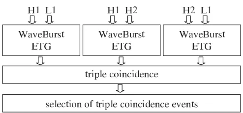
WaveBurst processes gravitational wave data from two interferometers at a time. As shown in Fig. 2 the analysis is performed over three LIGO detectors resulting in the pro-duction of triggers for three detector pairs. The three sets of triggers are then compared in a ‘‘triple-coincidence’’ step which checks for consistent trigger times and frequency components, as will be described in Section V B.
For each detector pair, the WaveBurst ETG performs the following steps: (a) wavelet transformation applied to the gravitational wave channel from each detector, (b)
tion of wavelet amplitudes exceeding a threshold, (c) iden-tification of common wavelet components in the two chan-nels, (d) clustering of nearby wavelet components, and (e) selection of burst triggers. During steps (a), (b) and (d) the data processing is independent for each channel. During steps (c) and (e) data from both channels are used.
The input data to the WaveBurst ETG are time series from the gravitational wave channel with duration of 120 seconds and sampling rate of 16 384 Hz. The data are first down-sampled to 8192 Hz. Using an orthogonal wavelet transformation (based on a symlet wavelet with filter length of 60 samples) the time series are converted into wavelet seriesWij, whereiis the time index andjis the wavelet layer index. Each wavelet layer can be asso-ciated with a certain frequency band of the initial time series. The time-frequency resolution of the WaveBurst scalograms is the same for all the wavelet layers (1=128 sec 64 Hz). Therefore, the wavelet series Wij can be displayed as a time-frequency scalogram consisting of 64 wavelet layers withn15 360pixels (data samples) each. This tiling is different from the one in the conven-tional dyadic wavelet decomposition where the time reso-lution adjusts to the scale (frequency) [29,38,39]. The constant time-frequency resolution makes the WaveBurst scalograms similar to spectrograms produced with win-dowed Fourier transformations.
For each layer we first select a fixed fractionPof pixels with the largest absolute amplitudes. These are calledblack pixels. The number of selected black pixels isnP. All other wavelet pixels are calledwhite pixels. Then we calculate rank statistics for the black pixels within each layer. The rankRijis an integer number from 1 tonP, with the rank 1 assigned to the pixel with the largest absolute amplitude in the layer. Given the rank of wavelet amplitudes Rij, the following nonparametric pixel statistic is computed
yij ln
R
ij nP
: (5.1)
For white pixels the value ofyijis set to zero. The statistic yij can be interpreted as the pixel’s logarithmic signifi-cance. Assuming Gaussian detector noise, the logarithmic
significance can be also calculated as
~
yij gPw~ij lnP ln
2=
p Z1 ~ wij
ex2=2dx
!
;
(5.2) where w~ij is the absolute value of the pixel amplitude in units of the noise standard deviation. In practice, the LIGO detector noise is not Gaussian and its probability distribu-tion funcdistribu-tion is not determineda priori. Therefore, we use the nonparametric statistic yij, which is a more robust measure of the pixel significance than y~ij. Using the in-verse function ofgPwithyijas an argument, we introduce thenonparametric amplitude
wijgP1yij; (5.3) and the excess power ratio
ijw2ij1; (5.4)
which characterizes the pixel excess power above the average detector noise.
After the black pixels are selected, we require their time-coincidence in the two channels. Given a black pixel of significance yij in the first channel, this is accepted if the significance of neighboring (in time) pixels in the second channel (y0ij) satisfies
y0i1jyij0 y0i1j> ; (5.5) whereis thecoincidence threshold. Otherwise, the pixel is rejected. This procedure is repeated for all the black pixels in the first channel. The same coincidence algorithm is applied to pixels in the second channel. As a result, a considerable number of black pixels in both channels produced by fluctuations of the detector noise are rejected. At the same time, black pixels produced by gravitational wave bursts have a high acceptance probability because of the coherent excess of power in two detectors.
After the coincidence procedure is applied to both chan-nels a clustering algorithm is applied jointly to the two channel pixel maps. As a first step, we merge (OR) the black pixels from both channels into one time-frequency plane. For each black pixel we define neighbors (either black or white), which share a side or a vertex with the black pixel. The white neighbors are calledhalopixels. We define a cluster as a group of black and halo pixels which are connected either by a side or a vertex. After the cluster reconstruction, we go back to the original time-frequency planes and calculate the cluster parameters separately for each channel. Therefore, there are always two clusters, one per channel, which form a WaveBurst trigger.
[image:8.612.53.300.42.157.2]The cluster parameters are calculated using black pixels only. For example, the cluster size k is defined as the number of black pixels. Other parameters which character-ize the cluster strength are the cluster excess power ratio and the clusterlogarithmic likelihoodY. Given a clusterC,
these are estimated by summing over the black pixels in the cluster:
X
ij2C
ij; Y X
ij2C
yij: (5.6)
Given the times ti of individual pixels, the cluster center time is calculated as
T X
ij2C tiw2ij
, X
ij2C w2
ij: (5.7)
As configured for this analysis, WaveBurst initially gen-erated triggers with frequency content between 64 Hz and 4096 Hz. As we will see below, the cluster size, likelihood, and excess power ratio can be used for the further selection of triggers, while the cluster time and frequency span are used in a coincidence requirement. The frequency band of interest for this analysis, 100 –1100 Hz, is selected during the later stages of the analysis.
There are two main WaveBurst tunable input parame-ters: the black pixel fraction P which is applied to each frequency layer, and the coincidence threshold . The purpose of these parameters is to control the average black pixel occupancyOP; , the fraction of black pixels over the entire time-frequency scalogram. To ensure robust cluster reconstruction, the occupancy should not be greater than 1%. For white Gaussian detector noise the functional form ofOP; can be calculated analytically. This can be used to set a constraint on P and for a given target OP; . If P is set too small (less then a few percent), noise outliers due to instrumental glitches may monopolize the limited number of available black pixels and thus allow gravitational wave signals to remain hidden. To avoid this domination of instrumental glitches, we run the analysis with P equal to 10%. This value of P together with the occupancy targetOP; of 0.7% defines the coincidence thresholdat 1.5.
All the tuning of the WaveBurst method was performed on the S2 playground data set (Sec. IV). For the selected values of P and , the average trigger rate per LIGO instrument pair was approximately 6 Hz, about twice the false alarm rate expected for white Gaussian detector noise. The trigger rate was further reduced by imposing cuts on the excess power ratio . For clusters of size k greater than 1 we requiredto be greater than 6.25 while for single pixel clusters (k1) we used a more restrictive cut ofgreater than 9. These criteria yielded mean trigger rates of 1.6 Hz for the (L1,H1) and (L1,H2) pairs and 1.2 Hz for the (H1,H2) pair. These rates varied by40%
over the course of the S2 run. The times and reconstructed parameters of WaveBurst events passing these criteria were written onto disk. This allowed the further processing and selection of these events without the need to reanalyze the full data stream, a process which is generally time and CPU intensive.
B. Triple coincidence
Further selection of WaveBurst events proceeds by iden-tifying triple coincidences. The output of the WaveBurst ETG is a set of coincident triggers for a selected interfer-ometer pair A; B. Each WaveBurst trigger consists of two clusters, one in A and one in B. For the three LIGO interferometers there are three possible pairs: (L1,H1), (H1,H2) and (H2,L1). In order to establish triple-coincidence events, we require a time-frequency coinci-dence of the WaveBurst triggers generated for these three pairs. To evaluate the time coincidence we first construct TAB TATB=2, i.e., the average central time of theA andBclusters for the trigger. Three such combined central times are thus constructed: TL1H1,TH1H2, andTH2L1. We then require that all possible differences of these combined central times fall within a time windowTw20 ms. This window is large enough to accommodate the maximum difference in gravitational wave arrival times at the two detector sites (10 ms) and the intrinsic time resolution of the WaveBurst algorithm which has a standard deviation on the order of 3 ms as discussed in Sec. VIII.
We apply a loose requirement on the frequency consis-tency of the WaveBurst triggers. First, we calculate the minimum (fmin) and maximum (fmax) frequency for each interferometer pairA; B
fminminfAlow; fBlow; fmaxmaxfhighA ; fBhigh; (5.8) where flow and fhigh are the low and high frequency boundaries of the A and B clusters. Then, the trigger frequency bands are calculated asfmaxfminfor all pairs. For the frequency coincidence, the bands of all three WaveBurst triggers are required to overlap. An average frequency is then calculated from the clusters, weighted by signal-to-noise ratio, and the coincident event candidate is kept for this analysis if this average frequency is above 64 Hz and below 1100 Hz.
The final step in the coincidence analysis of the WaveBurst events involves the construction of a single measure of their combined significance. As we described already, triple-coincidence events consist of three WaveBurst triggers involving a total of six clusters. Each cluster has its parameters calculated on a per-interferometer basis. Assuming white detector noise, the variableY for a cluster of sizekfollows a Gamma proba-bility distribution. This motivates the use of the following measure of thecluster significance:
ZYln X
k1
m0 Ym m!
!
; (5.9)
which is derived from the logarithmic likelihood Y of a cluster C and from the number kof black pixels in that cluster [28,29]. Given the significance of the six clusters, we compute the combined significance of the
coincidence event as
ZG ZLL11H1ZLH11H1ZHH22L1ZHL12L1ZHH11H2ZHH21H21=6; (5.10)
whereZA
AB(ZBAB) is the significance of theA(B) cluster for theA; Binterferometer pair.
In order to evaluate the rate of accidental coincidences, we have repeated the above analysis on the data after introducing an unphysical time-shift (‘‘lag’’) in the Livingston data stream relative to the Hanford data streams. The Hanford data streams are not shifted relative to one another, so any noise correlations from the local environment are preserved. Figure 3 shows the distribution of cluster significance (Eq. (5.9)) from the three individual detectors, and the combined significance (Eq. (5.10)), over
the entire S2 data set, for both zero-lag and time-lag coincidences. Using 46 such time-lag instances of the S2 playground data we have set the threshold on ZG for this search in order to yield a targeted false alarm rate of
10Hz. Without significantly compromising the pipeline sensitivity, this threshold was selected to belnZG>1:7. In the 64 –1100 Hz frequency band, the resulting false alarm rate in the S2 playground analysis was approxi-mately 15Hz. The coincident events selected by WaveBurst in this way are then checked for their waveform consistency using the r-statistic.
C.r-statistic test
The r-statistic test [30] is applied as the final step of searching for gravitational wave event candidates. This test reanalyzes the raw (unprocessed) interferometer data around the times of coincident events identified by the WaveBurst ETG.
The fundamental building block in performing this waveform consistency test is therstatistic, or the normal-ized linear correlation coefficient of two sequences, fxig and fyig (in this case, the two gravitational wave signal time series):
r
P
i
xixyiy
P
i
xix2
r P
i
yiy2
r ; (5.11)
where x and y are their respective mean values. This quantity assumes values between 1 for fully anticorre-lated sequences and1for fully correlated sequences. For uncorrelated white noise, we expect the r-statistic values obtained for arbitrary sets of points of lengthNto follow a normal distribution with zero mean and 1=pN. Any coherent component in the two sequences will cause rto deviate from the above normal distribution. As a normal-ized quantity, therstatistic does not attempt to measure the consistency between the relative amplitudes of the two sequences. Consequently, it offers the advantage of being robust against fluctuations of detector amplitude response and noise floor. A similar method based on this type of time-domain cross-correlation has been implemented in a LIGO search for gravitational waves associated with a GRB [7,40] and elsewhere [41].
As will be described below, the final output of the r-statistic test is a combined confidence statistic which is constructed fromr-statistic values calculated for all three pairs of interferometers. For each pair, we use only the absolute value of the statistic, jrj, rather than the signed value. This is because an astrophysical signal can produce either a correlation or an anticorrelation in the interfer-ometers at the two LIGO sites, depending on its sky position and polarization. In fact, the r-statistic analysis was done using whitened (see below) but otherwise
un-L1
Entries 2845
Mean 2.615 RMS 1.926
significance 1 10
events
1 10
2
10 Entries L1 2845
Mean 2.615 RMS 1.926
H1
Entries 2845
Mean 2.603 RMS 1.7
significance 1 10
events
1 10
2
10
H1
Entries 2845
Mean 2.603 RMS 1.7
H2
Entries 2845
Mean 2.572
RMS 1.826
significance 1 10
events
1 10
2
10 Entries H2 2845
Mean 2.572
RMS 1.826
L1xH1xH2
Entries 2845
Mean 2.235
RMS 0.9299
significance 1 10
events
1 10
2
10
L1xH1xH2
Entries 2845
Mean 2.235
[image:10.612.55.299.248.596.2]RMS 0.9299
calibrated data, with an arbitrary sign convention. A signed correlation test using calibrated data would be appropriate for the H1-H2 pair, but all three pairs were treated equiv-alently in the present analysis.
The number of pointsN considered in calculating the statistic in Eq. (5.11), or equivalently theintegration time , is the most important parameter in the construction of therstatistic. Its optimal value depends in general on the duration of the signal being considered for detection. Ifis too long, the candidate signal is ‘‘washed out’’ by the noise when computingr. On the other hand, if it is too short, then only part of the coherent signal is included in the integra-tion. Simulation studies have shown that most of the short-lived signals of interest to the LIGO burst search can be identified successfully using a set of three discrete integra-tion times with lengths of 20 ms, 50 ms, and 100 ms.
Within its LIGO implementation, ther-statistic analysis first performs data ‘‘conditioning’’ to restrict the frequency content of the data to LIGO’s most sensitive band and to suppress any coherent lines and instrumental artifacts. Each data stream is first band-pass filtered with an 8th-order Butterworth filter with corner frequencies of 100 Hz and 1572 Hz, then down-sampled to a 4096 Hz sampling rate. The upper frequency of 1572 Hz was chosen in order to have 20 dB suppression at 2048 Hz and thus avoid aliasing. The lower frequency of 100 Hz was chosen to suppress the contribution of seismic noise; it also defines the lower edge of the frequency band for this gravitational wave burst search, since it is above the lower frequency limit of 64 Hz for WaveBurst triggers. The band-passed data are then whitened with a linear predictor error filter with a 10 Hz resolution trained on a 10 s period before the event start time. The filter removes predictable content, including lines that were stationary over a 10 s time scale. It also has the effect of suppressing frequency bands with large stationary noise, thus emphasizing transients [39].
The next step in the r-statistic analysis involves the construction of all the possible r coefficients given the number of interferometer pairs involved in the trigger, their possible relative time-delays due to their geographic sepa-ration, and the various integration times being considered. Relative time delays up to10 msare considered for each detector pair, corresponding to the light travel time be-tween the Hanford and Livingston sites. Future analyses will restrict the time delay to a much smaller value when correlating data from the two Hanford interferometers, to allow only for time calibration uncertainties. Furthermore, in the case of WaveBurst triggers with reported durations greater than the integration time , multiple integration windows of that length are considered, offset from the reported start time of the trigger by multiples of=2. For a given integration window indexed by p(containing Np data samples), ordered pair of instruments indexed byl; m
lm, and relative time delay indexed by k, the r-statistic valuejrkplmjis calculated. For eachplm
combi-nation, the distribution of jrk
plmj for all values of k is compared to the null hypothesis expectation of a normal distribution with zero mean and 1=pNp using the Kolmogorov-Smirnov test. If these are statistically consis-tent at the 95% level, then the algorithm assigns no sig-nificance to any apparent correlation in this detector pair. Otherwise, a one-sided significance and its associated logarithmic confidence are calculated from the maximum value ofjrk
plmjfor any time delay, compared to what would be expected if there were no correlation. Confidence values for all ordered detector pairs are then averaged to define the combined correlation confidence for a given integration window. The final result of the r-statistic test, , is the maximum of the combined correlation confidence over all of the integration windows being considered. Events with a value ofabove a given threshold are finally selected.
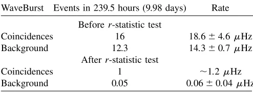
Ther-statistic implementation, filter parameters, and set of integration times were chosen based on their perform-ance for various simulated signals. The single remaining parameter, the threshold on, was tuned primarily in order to ensure that much less than one background event was expected in the whole S2 run, corresponding to a rate of O0:1Hz. Since the rate of WaveBurst triggers was approximately15Hz, as mentioned in Sec. V B, a rejec-tion factor of around 150 was required.
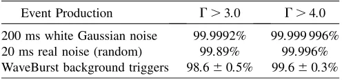
[image:11.612.314.562.657.715.2]Table I shows the rejection efficiency of the r-statistic test for two thresholds on when the test is applied to white Gaussian noise (200 ms segments), to real S2 inter-ferometer noise at randomly selected times (200 ms seg-ments), and to the data at the times of time-lag (i.e., background) WaveBurst triggers in the S2 playground. In the first two cases, 200 ms of data was processed by the r-statistic algorithm, whereas in the latter case, the amount of data processed was determined by the trigger duration reported by WaveBurst. The table shows that random detector noise rarely produced a value above 3.0, but the rejection factor for WaveBurst triggers was not high enough. Athreshold of 4.0 was ultimately chosen for this analysis, yielding an estimated rejection factor of250for WaveBurst triggers. For all of the simulated waveforms considered in Sec. VIII, the r-statistic waveform consis-tency test with>4:0represents a sensitivity that is equal to or better than that of the WaveBurst ETG. As a result of this, the false dismissal probability of the r-statistic test does not impair the efficiency of the whole pipeline.
TABLE I. Percentage of S2 background triggers rejected by therstatistic for two different thresholds on.
Event Production >3:0 >4:0
VI. VETOES
We performed several studies in order to establish any correlation of the triggers produced by the WaveBurst search algorithm with environmental and instrumental glitches. LIGO records hundreds of auxiliary readback channels of the servo control systems employed in the instruments’ interferometric operation as well as auxiliary channels monitoring the instruments’ physical environ-ment. These channels can provide ways for establishing evidence that a transient is not of astrophysical origin, i.e., a glitch attributed to the instruments themselves and/or to their environment. Assuming that the coupling of these channels to a genuine gravitational wave burst is null (or below threshold within the context of a given analysis), such glitches appearing in these auxiliary channels may be used to veto the events that appear simultaneously in the gravitational wave channel. The WaveBurst pipeline used in this S2 search was a multi-interferometer search method which did not produce any single-interferometer triggers. Thus, although environmental and instrumental disturban-ces would be expected to affect only one site or the other, for this analysis it was most practical and direct to use WaveBurst triple-coincidence triggers to evaluate potential vetoes. Any trigger coincident with a vetoed time interval was simply removed. An option existed of rerunning WaveBurst with the vetoed time intervals excluded, but this would have fragmented the data set and introduced edge effects and was thus not pursued.
Given the number of auxiliary channels and the parame-ter space that we need to explore for their analysis, an exhaustivea prioriexamination of all of them is a formi-dable task. The veto study was limited to the S2 play-ground data set and to a few tens of channels thought to be most relevant. Several different choices of filter and threshold parameters were tested in running the glitch finding algorithms. For each of these configurations, the efficiency of the auxiliary channel in vetoing the event triggers (presumed to be glitches), as well as the dead-time introduced by using that auxiliary channel as a veto, were computed and compared to judge the effectiveness of the veto condition.
Another important consideration in a veto analysis is to verify the absence of coupling between a real gravitational wave burst and the auxiliary channel, such that the real burst could cause itself to be vetoed. The ‘‘safety’’ (ab-sence of such a coupling) of veto conditions was evaluated using hardware signal injections (described in Sec. VIII), by checking whether the simulated burst signal imposed on the arm length appeared in the auxiliary channel. Only one channel, referred to as AS_I, in the L1 instrument derived from the antisymmetric port photodiode with a demodu-lation phase orthogonal to that of the gravitational wave channel, was found to be ‘‘unsafe’’ in this respect, con-taining a small amount of the injected signal.
None of the channels and parameters we examined yielded an obviously good veto (e.g., one with an effi-ciency of 20% or greater and a dead-time of no more than a few percent) to be used in this search. Among the most interesting channels was the one in the L1 instrument that recorded the DC level of the light coming out of the antisymmetric port of the interferometer, referred to as AS_DC. That channel was seen to correlate with the gravi-tational wave channel through a nonlinear coupling with interferometer alignment fluctuations. A candidate veto based on this channel was shown to be able to reject
15% of the triggers, but with a non-negligible dead-time of 5%. Finding no better option, we decided not to apply any a priorivetoes in this search, judging that the effect on the results would be insignificant.
Although none of the auxiliary channels studied in the playground data yielded a compelling veto, these studies provided experience applicable to examining any candi-date gravitational wave event(s) found in the full data set. A basic principle established for the search was that a statistical excess of zero-lag event candidates (over the expected background) would not, by itself, constitute a detection; the candidate(s) would be subjected to further scrutiny to rule out any environmental or instrumental explanation that might not have been apparent in the initial veto studies. As will be described in the next section, one event did survive all the predetermined cuts of the analysis but subsequent examination of auxiliary channels identi-fied an environmental origin for the signal in the two Hanford detectors.
VII. SIGNAL AND BACKGROUND RATES
In the preceding section we described the methods that we used for the selection of burst events. These were applied to the S2 triple-coincidence data set excluding the playground for a total of 239.5 hours (9.98 days) of observation time. Every aspect of the analysis discussed from this point on will refer only to this data set.
A. Event analysis
The WaveBurst analysis applied to the S2 data yielded 16 coincidence events (at zero-lag). The application of the rstatistic cut rejected 15 of them, leaving us with a single event that passed all the analysis criteria.
make a measurement of the accidental rate of coinci-dences, i.e., the background. This step size was much larger than the duration of any signal that we searched for and was also larger than the autocorrelation time-scale for the trigger generation algorithm applied to S2 data. This can be seen in Fig. 4 where a histogram of the time between consecutive events is shown for the double and their resulting triple-coincidence WaveBurst zero-lag events before any combined significance orr-statistic cut is applied. These distributions follow the expected expo-nential form, indicating a quasistationary Poisson process. The background events generated in this way were also subjected to ther-statistic test in an identical way with the one used for the zero-lag events. Each time-shift experi-ment had a different live-time according to the overlap, when shifted, of the many noncontiguous data segments that were analyzed for each interferometer. Taking this into account, the total effective live-time for the purpose of
measuring the background in this search was 391 days, equal to 39.2 times the zero-lag observation time.
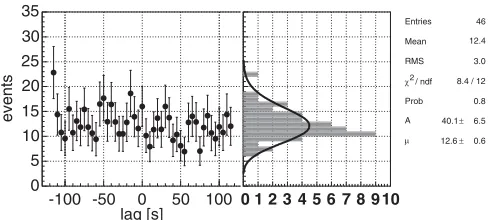
[image:13.612.318.562.46.156.2]A plot of the measured background events found in each of the 46 time-lag experiments, before the application of the r-statistic, is shown in Fig. 5 as a function of the lag time. These numbers of events are corrected so that they all correspond to the zero-lag live time. A Poisson fit can be seen in the adjacent panel; the fit describes the distribution of event counts reasonably well.
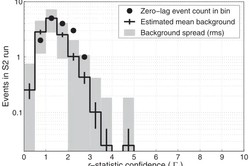
Figure 6 shows a histogram of the values, i.e., the multi-interferometer combined correlation confidence, for the zero-lag events. The normalized background distribu-H1H2
Entries 346262 / ndf
2
χ 142 / 104 Constant 9.928 ±0.015 Slope -0.2399 ± 0.0012
time between consecutive events, seconds
0 10 20 30 40 50 60
events
1 10
2
10
3
10
4
10
5
10 H1H2
Entries 346262 / ndf
2
χ 142 / 104 Constant 9.928 ±0.015 Slope -0.2399 ± 0.0012
H1L1
Entries 355456 / ndf
2
χ 108 / 98
Constant 10.1 ±0.0 Slope -0.2701 ± 0.0015
time between consecutive events, seconds
0 10 20 30 40 50 60
events
1 10
2
10
3
10
4
10
10 H1L1
Entries 355456 / ndf
2
χ 108 / 98
Constant 10.1 ±0.0 Slope -0.2701 ± 0.0015
L1H1H2
Entries 2141
/ ndf 2
χ 27.17 / 19
Constant 6.457 ±0.032 Slope -0.003761 ± 0.000091
time between consecutive events, seconds
0 200 400 600 800 1000 1200 1400 1600 1800 2000
events
1 10
2
10
3
10 L1H1H2
Entries 2141
/ ndf 2
χ 27.17 / 19
Constant 6.457 ±0.032 Slope -0.003761 ± 0.000091
FIG. 4. Time between consecutive WaveBurst events (prior to the application of ther-statistic test). The top two panels show the distributions for double-coincidence H1-H2 and H1-L1 triggers, respectively. The triple-coincidence events, shown in the bottom panel, are reasonably well described by a Poisson process of constant mean. The exponential fits are performed for time delays greater than 4 s.
lag [s]
-100 -50 0 50 100
events
0 5 10 15 20 25 30 35
0 1 2 3 4 5 6 7 8 9 10
Entries 46
Mean 12.4
RMS 3.0
/ ndf 2
χ 8.4 / 12
Prob 0.8
A 40.1 ± 6.5
µ 12.6 ± 0.6
FIG. 5. WaveBurst event count (prior to the r-statistic test) versus lag time (in seconds) of the L1 interferometer with respect to H1 and H2. The zero-lag measurement, i.e., the only coinci-dence measurement that is physical, is also shown. Because of the fragmentation of the data set, each time-lag has a slightly different live-time; for this reason, the event count is corrected so that they all correspond to the zero-lag live-time. A projection of the event counts to a one-dimensional histogram with a Poisson fit is also shown in the adjacent panel.
0 1 2 3 4 5 6 7 8 9 10 0.1
1 10
r−statistic confidence ( Γ )
Events in S2 run
Zero−lag event count in bin Estimated mean background Background spread (rms)
[image:13.612.53.296.290.632.2]One zero−lag event with 4 < Γ < 4.5
FIG. 6. Circles: histogram ofr-statistic confidence value () for zero-lag events passing the WaveBurst analysis. Stair-step curve: mean background per bin, estimated from time lags, for an observation time equal to that of the zero-lag analysis. The black error bars indicate the statistical uncertainty on the mean background. The shaded bars represent the expected root-mean-square statistical fluctuations on the number of background events in each bin.
[image:13.612.319.560.449.618.2]