Approximating distributional behaviour of LTI differential systems using Gaussian function and its derivatives

(1)

City, University of London Institutional Repository

Citation

: Pantelous, A., Karcanias, N. & Halikias, G. (2012). Approximating distributional

behaviour of LTI differential systems using Gaussian function and its derivatives.

International Journal of Control, 85(7), pp. 830-841. doi: 10.1080/00207179.2012.667881

This is the accepted version of the paper.

This version of the publication may differ from the final published

version.

Permanent repository link:

http://openaccess.city.ac.uk/7295/

Link to published version

: http://dx.doi.org/10.1080/00207179.2012.667881

Copyright and reuse:

City Research Online aims to make research

outputs of City, University of London available to a wider audience.

Copyright and Moral Rights remain with the author(s) and/or copyright

holders. URLs from City Research Online may be freely distributed and

linked to.

(2)

1

Approximating distributional behaviour of LTI differential

systems using Gaussian function and its derivatives

Athanasios A. Pantelous1*, Nicos Karcanias2and George Halikias2

1

Department of Mathematical Sciences, University of Liverpool, UK

2

School of Engineering and Mathematical Sciences, City University, UK

Abstract

The paper is concerned with the approximation of the destributional behaviour of linear,

time-invariant (LTI) systems. First, we review the different types of approximations of

distributions by smooth functions and explain their significance in characterizing

sys-tem properties. Secondly, for controllable LTI differential syssys-tems, we establish an

inte-resting relation between the time and volatility parameters of the Gaussian function and

its derivatives in the approximation of distributional solutions. An algorithm is then

proposed for calculating the distributional input and its smooth approximation which

minimizes the distance to an arbitrary target state. The optimal choice of the volatility

parameter for the state transition is also derived. Finally, some complementary distance

problems are also considered. The main results of the paper are illustrated by numerous

examples.

AMS (Classification): 93C05, 34K45, 34A37

Keywords: Linear Systems; Approximating Distributional Behaviour; Gaussian Func-tion and its Derivatives

*Corresponding Author: Dr Athanasios Pantelous, Department of Mathematical Sciences, University of

(3)

2

1. Introduction

The use of distributions in the study of LTI differential system problems is a

well-established subject going back to [3, 4-6, 8, 10, 12, 14-21] and references therein. The

work so far has dealt with the characterisation of basic system properties such as infinite

poles and zeros [17, 18] for regular and singular (implicit) systems, as well as the study

of fundamental control problems where the solution is expressed in terms of

distribu-tions. Typical problems are those dealing with the notions of almost



A B,



-invariance and almost controllability subspaces [12], [20].

Indeed, the study of distributional solutions plays a key role in many areas in

sys-tems and control such as:

(i) Controllability, Observability.

(ii) Infinite zero characteristic behaviour.

(iii) Almost invariant subspaces, almost controllability spaces.

(iv) Dynamics of singular systems etc.

The distributional characterization is also linked to the solution of a number of

con-trol problems. The solution of these problems has only theoretical significance, given

that distributions cannot be constructed and only smooth functions can be implemented.

The idea of approximating distributional inputs with smooth functions that achieve a

similar control objective was first introduced by Gupta and Hasdorff [10] (see also

[11]).

In the present paper, which actually extends and provides a rigorous reformulation

of the early ideas presented in [10], we consider the problem of approximating Dirac

distributions with smooth functions of infinite support, and more specifically using the

Gaussian distribution and its derivatives. Analytically, in Section 2 we present the

prob-lem formulation for a LTI differential system. In Section 3 we provide a brief review of

the different types of approximations of distributions by smooth functions and explain

(4)

3 system is controllable, and under this assumption we establish an interesting connection

between a time-parameter t and a volatility parameter  of the Gaussian density func-tion used in the approximafunc-tion. It turns out that the fracfunc-tion t/ can be fixed (to a suf-ficiently large value) and in this case parameter t (or  ) controls the state-transition time and the accuracy of the approximation (which can be interpreted probabilistically).

A new algorithm is proposed for calculating the smooth input signal that approximates

the distributional input which transfers the origin of the state-space to an arbitrary target

point (subject to a controllability assumption) and the distance (Euclidean norm)

be-tween the actual terminal state and the target state; this distance is subsequently

mini-mized subject to magnitude constraints imposed on the coefficients of the control signal.

Finally, in Section 5 we define the distance from the origin using the Euclidean norm.

Moreover, we consider the problem of maximising the distance from the origin with

constrained input. Section 6 concludes the paper.

2. Problem Definition

We consider the linear time invariant (LTI) system

 

o

 

x t Ax t bu t , (2.1)

where x t

 





,



n1;



(smooth function over the field    or , whose elements belong to the algebra 



n1;



), and u to

 

n1 (where n1 is the space

of Dirac distribution having derivatives up to an order n1) are the state vector, and the impulsive input, respectively andA



n n R ;



, b



n1;R



. Following also [10], we assume that A is simple and expressed as



1, 2,..., n



Adiag    , (2.2)

where _i _j 0 for every in

 (n:



1, 2,,n



). This assumption can be relaxed, see

(5)

4 It is assumed that the input to the LTI is a linear combination of Dirac  -function

and its first n1 derivatives, i.e.

 

1 0

n k

o k

k

u t a t

 



_

, (2.3)

where  k or

k k

d dt



is the kth derivative of the Dirac  -function, and a_k for in_o 

(n_o: {0,1, n1}

 ) are the magnitudes of the delta function and its derivatives. We

T n

 

0 by the action of the control input defined in (2.3) is that

 

1 0

n

k k k

x t   t

 



_

where the coefficients _k, kn_o

 , are the components of x

 

0



along the directions { ,b Ab A b, 2 ,,A bn1 }, respectively, defined according to some projections law.

In the next section, some background results as a brief review on the approximation

of Dirac delta function are presented.

3. Approximations of Dirac Delta Function

The approximation of distributions by smooth functions is a problem which has

been considered in the literature. In this section, we review the main results in this area

(6)

5 their derivatives. If the standard approximating technique of the Dirac  -function is

followed, (see e.g. [7-8, 11-13, 22]), the change of the state in some minimum practical

time depends mainly on the accuracy of the approximations that have been generated.

The relation between the type of approximation used and the duration of the resulting

state-transition is one of the important issues considered in this section.

The Dirac  -function can be viewed as the limit of a sequence of functions

 

0

lim _a

a

t t

 



 , (3.1)

where _a

 

t is referred to as a nascent delta function. The limit is in the sense that

   

 

0

lim _a 0

a  t f t dt f

 







. (3.2)

These properties can be approximately enforced by using a smooth, finite

approxi-mation of the Dirac distribution. Such approxiapproxi-mations have additional advantages.

Ap-proximating the Dirac distribution by a smooth function may actually be a better

repre-sentation of the solution sought in a particular problem, especially if the effective width

of the approximation function can be coupled to the physics of the problem. Following

Cohen and Kirschner [7], a suitable approximating function, which is convenient for

computations, should satisfy the following properties everywhere on the domain under

consideration:

1. Its limit with some defining parameter is the Dirac distribution (see eq. (3.1)).

2. It is positive, decreases monotonically from a finite maximum at a source point (for instance 0), and tends to zero at the domain’s extremes.

3. Its derivative exists and is a continuous function.

4. It is symmetric about the source point, for instance 0 (see eq. (3.1) and (3.2)).

(7)

6 Next, we discuss the approximation of the Dirac delta function by functions having

infinite support.

3.1. Infinite Time-support approximations

The choice of the “best” nascent delta function depends on the particular

applica-tion. Choices which have proved useful in applications are listed below and include the

Gaussian and Cauchy distributions, the rectangular function, the derivative of the

sig-moid (or Fermi-Dirac) function, the Airy function, etc, see for instance [8, 11, 13, 22];

for approximations based on finite difference methods see [2]:

● The Cauchy distribution:

 

2 2

1 1 ikt ak

a

t e dk

a t



 

 _ 

 





,

● The rectangular function:

 



/



1 sin

2 2

ikt a

rect t a ak

t c e dk

a



 

 

 

  _ _

 



,

where

 

1, 1 1.

0, 1

t rect t

t

   

  

 



● The partial derivative of the sigmoid (or Fermi-Dirac) function,

 

/ /

1 1

a t t t a t t a

e e

   _  

  ,

● The Airy function

 

1

a i

t

t A

a a

(8)

7 The finite difference formulae may be easily converted into sequences that

ap-proximate the derivatives of the Dirac delta function in one dimension [2]. Recall the

definition of the rectangular function

 

1 , 2 2 0, 2 a a a t a t a t           _  

, (3.3)

which approaches 

 

t as a0. An expression for the derivatives of 

 

t is given by

 





0 0 0 1 lim , k k k

j a j

k _a

j h

d

x a x b h

dx   h 

  _{ }   __{ }  _     



 (3.4)

where xt_ot, the a_j are appropriate constants defining the finite differences [2], and

 

|

 

1

 

|

o

k k

k

t t x

k k

d d

u u

du     du  .

Expression (3.4) is exactly what we would obtain by making the substitution

 

a

 

f t  t in the following finite difference approximation for the kth_{derivative of}

a smooth test function f evaluated at t_o :

 





0 1 | o k k k

t t j o j

k

j d

f t a f t b h dt  h 

 

_{ } 

 



. (3.5)

Note that a_j and b_j are suitably chosen constants and (3.5) becomes exact in the limit h0. Note also that

 

₀





 

0 1 | lim o k k k

t t j o j

k _h

j

d

f t a t t b h f t dt

dt h 

           __{ }   _     

 



. (3.6)

(9)

8 In our case the Gaussian distribution may be considered as a good approximation of

the Dirac distribution on an infinite domain.

3.2 Input signal structure

Since our time-domain is infinite, the Gaussian distribution, i.e.

 

2/2 2

0 0

1 1

lim lim

2

t t

t e 

 



   



 

 

  _{  }

  where

 

2

/ 2

1 :

2

x

x e





  (3.8)

is considered. Hence, the approximate expression for the input signal (2.3) is given by

 

1

1 0

1

,

n

k k k k

t u_ t a

 



 

 

  _ _

 



(3.9)

where

 

( / )

i i

i

t d t

d t

  

 

   

 _ __ __ _

     

.

The impulsive response of the system is recovered in the limit:

 

0

lim

o

u t u_ t



 . (3.10)

A natural question arising in the context of the zero-time state-transition problem

considered in this work is why attention is restricted to impulsive control signals

ex-pressed as a sum of Dirac delta functions (and its derivatives). The answer to this

ques-tion involves the idea of single-layer distributions [8, 13, 22] which is briefly

intro-duced in the next few paragraphs:

Lemma 3.1 [22] If  is a bounded closed set in  and  is a neighbourhood of , then there exists a function such that n1 on , n0 outside , and 0 n 1 over

(10)

9

Definition 3.1 Let  be a piecewise regular curve in  and  is a locally integrable function defined on . The linear continuous functional _S on the space  of infi-nitely differentiable complex-valued functions on  with compact support is defined as

   

, ,

S

S S

  

_

    



  and is called single (or simple) layer on  with density  . 

Note that _S

_{ }

_

_{  }

S

x x S

 

_

     .

Definition 3.2 Let  be a piecewise regular curve in  and _S. The linear continu-ous functional d dt/



S



on the space  of infinitely differentiable complex-valued

functions on  with bounded support is defined as





 





/ _S ,

S

d x

d dt S

dt

       

 

_

In this section, we attempt to answer the following question: “What are the

coeffi-cients a , k_k n

(11)

10

signal defined in equation (2.3) transfers the state from x

 

0 to x

 

0 ?” In attempt-ing to answer this question the followattempt-ing standard result is significant.

Lemma 4.1 [11] The solution of system (2.1) is given by

 

,

t

At A

o

x t e e bu  d





_

(4.1)

where u_o

 

 is defined in equations (3.9) and (3.10). 

Remark 4.1 Recall that for simplicity it is assumed that matrix A is diagonal with dis-tinct eigenvalues. This reduces the complexity of various mathematical expressions

and the number of technicalities involved, without introducing any real loss of

general-ity. The general case can be tackled by defining a n n non-singular similarity

trans-formation Q



v v₁, ₂,,v_n







n n ;



that takes A_{into the Jordan canonical form.}

The solution of system (2.1) to the input defined in equations (3.9) and (3.10) is

 

0

lim ,

t

At A

x t e e bu_ d

  

 



 

 _ _







or equivalently

 

1

1 0

0

1

lim .

t _n

k

At A

k k k

x t e e b a d



 

 

 

 

 

 _ _ 

 _  _ _ _

 









(4.2)

As  0, the energy of the input signal “concentrates” around  0. Hence the

zero-time state-transition problem involves setting t0 and selecting the coefficients

k

a so that (an arbitrary) x(0 ) n is reached (recall that controllability of the pair ( , )A b is assumed).

(12)

11





2

1 2

1

/ ,

2

t t  e 



      

 

and its derivatives tend to zero very strongly with t/  . Define t/ K t

_

,

_

and assume that t is fixed to a positive value, so that K t



,



  as  0. Then,



/





,



,  0,

K t t K t



 



  

and its derivatives

 



/



 



,



,  0

K t

k k

t K t



 



   , kn_o

 .

where  0

_

t/

_



_

t/

_

.

A suitable choice of K t



,



depends on the choice of the transition time-variable

t and the volatility-parameter . In practice, t can be fixed, since we can pre-define the duration of the (almost zero) transition between the initial and final (target) state of

the system when solving the (almost) zero-time state transition problem (e.g., we can

select t to be of the order of t106seconds, say). This is the approximate version of the exact problem and can be formulated as follows:

For a fixed value of the time parameter tt* and a fixed  0 determine

 





* * *

ˆ

sup R : x t x t ,

   _  

(4.3)

where

 

*

x t is the target state and _ˆ

 

*

x t is the actual terminal state resulting from the approximation of the input signal, see equation (4.1).

This is in the form of a distance-approximation problem. Roughly, for a fixed

state-transition time-duration, we seek the “smoothest” input signal for which the error

toler-ance of the disttoler-ance between the target and actual terminal state is kept within a

pre-defined level . Note, that since this distance tends to zero as  0_{and the only}

(13)

deriva-12 tives, an alternative equivalent formulation of the problem is to determine (for a fixed

value tt*),

 













* *

sup R : k K t , _k,k n_o ,

        

where the _k are suitable positive constants.

The following lemma is required for subsequent developments. The objective is to

develop approximation bounds for the terminal state when the impulsive inputs in

equa-tion (4.1) are substituted by their smooth approximaequa-tions.

Lemma 4.2Consider u t_( ) defined in equations (3.9). Then

 

  2 2 1 1 1 1 2 1 0 1 , i i

t n k m k

k m

t i k

k k m i i

k m

t t

e  u_  d a e    e    

                         _ _  _ __  _  __          





(4.4)



 

_

   , x



0,1 .



Proof Substituting expression (3.9) into the integral i

 

t

e u_  d





, we obtain

 





 





1 1 1 1 0 0 / / . i i k

t n n t

k k k k k k k a

e     d a e     d

              





Consider first the term corresponding to k 0,





1 2 2 1 2 1 2 2

1 2 2 2 / 1 . 2 i i t t i t

e d e  e d e 

           _  _ _{ }        _  _        _ _    _  _  



Consider next the term corresponding to k1. Integration by parts and using the

equa-tion above gives













2

/ 1 /

/

i i i

t t

t i

e     d e      e     d

(14)

13





2 2 1 1 2 1

it / .

i i

t e  t  e    

          _  _   Similarly,





















2 2

3 2 2

1

2 ₂ 1 2

/ 1 /

/

1 1

/ / .

i i i

i

t t

t i

t

i i i

e d e e d

t

e t t e 

                                                    _    _  _  _    



A recursive application of this procedure gives

 





  2 2

1

1 ₂ 1

1 1 1 / 1 , i i k t k k m

t m k k

i i i

k k m

m

t t

e     d e    e    

                _ _ _ _   _ _  _  _    





from which the result follows. 











2 2 0 1 1 2 1 /

0 , .

i

k

i i

k

e     d  e   K              



Combining expressions (4.2) and (4.4) then gives









0 ,  1 2 2





1

1 2

0

0 , i i 0 , ,

n K

k

i i i k i

k x K   b e     K    a 

 _ 

  



  

_

(4.5)

for i1, 2,,n. The approximate almost zero-time state-transfer problem can now be

defined as follows: Suppose that parameters (0 , ) 

have been chosen so that

 

_

_

 

_

_





0 / 0 , 0

k k

K

 

 

   , kn_o

 . Then, given

 

0

n x 

 determine real

sca-lars a_k, kn_o

 such that (4.5) are satisfied with equality for all i{1, 2,, }n . Note that

(15)

14 above equation becomes exact; in this case we also have that x_i(0 ) xˆ_i(0 )

 ,









1

0 , _i 1

K   

 

   , and

 

0 1

0

ˆ 0 i , 1, 2, ,

n k

i i k i

k

x b e  a  i n

 



_

 

so that

 

2 2





 

1

2 _ˆ

0 i 0 , 0 , 1, 2, , .

i i i

x  e    K     x  i n

    

The following Theorem now follows.

Theorem 4.1 Let Adiag

_

 ₁, ₂,_n

_

_with _i _j for i j_, b



b₁ b₂  b_n



T

and assume that the pair ( , )_{A b is controllable. Let also}Bˆdiag



1/ ,1/b₁ b₂,,1/b_n



and denote by V V



 ₁, ₂,...,_n



the Vandermonde matrix





2 1

1 1 1

2 1

2 2 2

1 2 2 1 1 1 , ,..., . 1 n n n n

n n n

V V                                   

Then the coefficient vector a



a_o a₁  a_n_₁



T of the input signal defined in (3.9) which solves the almost zero-time state-transfer problem is given by

 

1 A0 _{ˆ ˆ 0}1

aV e  B x  , (4.6)

where

 













2 2 1 1 2 0 , ˆ 0 0 , i i i i x K x

e   K

          

 , in.

 (4.7)

(16)

15

2 2

1 0

/ 2 1 0

(0 ) ˆ (0 )

(0 )

i

i n

k i

i i k

k _i

x

x b e a

e



 





  



 



 

 



for in

.

Thus we can write ˆ 0

 

ˆ A0

x  Be Va or equivalently (4.6). Note that the indicated

in-verses V1 and Bˆ1 exist due the assumption that the eigenvalues of A are distinct, and the assumed controllability of ( , )A b , respectively. 

Ideally the parameters t* 0 and  should be chosen so that the distance

 

*

 

*









2

1 2

ˆ , ˆ ,

n

i i

i

x t x t 

_

_ _x K t   x K t   _

is “small”. Clearly the distance is zero provided that K t



,



is selected so that









2 2

1

1 ₂

, _i i 0

K t    e  



   

(4.8)

for all i which requires  0_{, in which case (4.8) implies that}







K t

x dx



 



,

which is the cumulative distribution function (cdf) of a random variable X ~N(0,1)

evaluated at the upper limit of the integral K t



,



, denoting the probability that



,



X K t  . In practice, if | _i |1 for all i, we can assume that equation (4.8) is

ap-proximately satisfied if K₀  K t



,



3.9 (in which case 1



K₀



 1 104). Thus, a reasonable choice for the volatility parameter is * K t01 * 0.256t*



(17)

16 The results of the section are summarised in the following algorithm.

Algorithm TIAZT (Transfer In Almost Zero Time)

1st Step: Define the terminal (target) state of the transitionx

 

0 .

2nd Step: Using the required transition time t*



0



define the optimal volatility parameter* 0.256t*.

3rd Step: Finally, the coefficients if the input signal a



a_o a₁  a_n_₁



T de-fined in equation (3.9) are obtained by (4.6), i.e. aV e1  A0B xˆ ˆ 01

 

 where all variables are defined in Theorem 4.1.

Remark 4.4 From the control viewpoint it is important to choose an appropriate time duration for the state transition. This ultimately depends on the type of application, e.g.

due to control signal magnitude or “slew-rate” limitations. It is clear from the imposed

proportionality *K t₀1 * that increasing the duration of the state-transition results is “smoother” input signals, which is often desirable. For example, if the system operates

in a feedback loop (in which case the input signal is generated by a feedback controller),

highly discontinuous signals typically correspond to system overdesign (e.g. excessive

closed-loop bandwidth) and may have detrimental effects on the stability and

perform-ance characteristics, e.g. in terms of reduced robust stability margins and sensor noise

amplification.

Example 4.1 (See Gupta, 1966) Consider the system

 

1 1

2 2

2 0 1

0 3 2 o

x t x t

u t

x t x t



      

 

 _   _    

   

where x t

 

and u t_o

 

are the state and the input signals, respectively. Suppose we wish

106



4. The inverse of the Vandermonde matrix is:





1

1 1 1 2 3 2

2, 3 .

1 3 1 1

V V



 _  _{ } _   _  

 _   _ 

   

Thus, the coefficient vector a



a₀ a₁



T is calculated as:

1 -6

-6 1

3 -2 exp(2 10 ) 0 1 0 3 5

1 -1 0 exp(3 10 ) 0 2 4 1

o

a a

a



  

         

_ __ __ _ _ _{  }_{ } 

       

   

.

5. Distance Problems

5.1. Distance from the origin in state-space

In this section, we define the distance from the origin corresponding to a state

tran-sition of the system (2.1) from the zero (or ground) state, x

 

0 



0 0  0



T.

Us-ing the Euclidean norm this is defined as

 

2

   

 

2 2

1

0 0 T 0 0 n _i 0

i

r x  x  x  x  x 



  

_

 , (5.1)

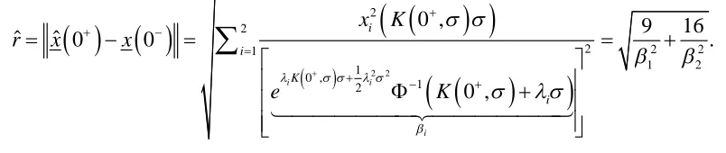
(see Fig 1). The time interval of the transition has been defined in previous sections as

(19)

18 However, if the Dirac delta function and its derivatives are replaced by smooth

sig-nals (Gaussian distribution function and its derivatives), this target state will not be

reached exactly, in general. The distance in terms of the target state xˆ 0

 

 is defined as

 













2 2 2 2 2 2 1 1 1 0 ,

ˆ ˆ 0 ,

0 , i i n n i i i i x K r x

e  K

            _ _   





where (4.7) has been used. Note that fixing K t

_

,

_

and taking  0, we get rˆr.

Example 5.1 Consider the system:

 

1 1 2 2

2 0 1

,

0 3 2 o

x t x t

u t

x t x t

           _   _            

where x t

 





R,



2 1; R



and u t_o

 

are the state vector and the input,

respec-tively. Let x









2 2 2 2

2 2 2

1 1 2 1 0 , 1 2

0 , ₉ ₁₆

ˆ ˆ 0 0 .

0 , i i i i i K i x K

r x x

e     K

                        _ _       





[image:19.595.97.499.571.656.2]

As  ₁, ₂1, rˆr 5.

Fig. 1: 2-ball with centre x

 

0 and radius rˆ

 

0 x 

S

r

(20)

19

5.2 Maximum distance from the origin with constrained input

Here we assume that the system (2.1) starts from the zero state at time t 0 and consider the problem of maximising the distance to the terminal state in an (almost)

zero-time state transition. This problem of course makes sense if the input signal is

con-strained in some sense. Here we impose constraints on the coefficient vector of the input

signal a



a₀ a₁  a_n_₁



Tin terms of the Euclidian and the infinity norms.

Lemma 5.1 Let i 0, i1, 2,,n. Then





1 1

1 max , 1

p n

n n

i i

i  n i 

 

  



for all

1, 2, ,

p  n.

Proof Define function 1

1

( ) n _i x

i

f x 

_

_   which can be written as ( 1)

1

( ) n m xi

i

f x 

_

_e  by

setting m_i ln_i . Since ( ) n₁ 2 m xi( 1) 0

i i

f x 



_ m e   for all x, function is convex for all x and specifically in the interval 1xn. Thus f x( ) attains its maximum at an edge of the interval 1xn, i.e.









1 1

1

1 max ( ) max (1), ( ) max , 1 ,

p n

n n

i x n i

i  f x f f n n i 

 

 

    



for every p1, 2,,n as required. 

Theorem 5.1 Let Adiag

_

 ₁, ₂,_n

_

_,b

_

b₁ b₂  b_n

_

T and assume that the pair

( , )_{A b is controllable. Define} Bˆ diag



1/ ,1/b₁ b₂,,1/b_n



and denote by V 



1, 2,..., n



V    the Vandermonde matrix





2 1

1 1 1

2 1

2 2 2

1 2

2 1

1 1

, ,..., .

1

n n n

n

n n n

V V

        

  

 



 

 

 

 

 

  

(21)

20

Let a



a_o a₁  a_n_₁



T be the coefficient vector of the input signal u t_o( )

 

1 0

n _i

i i a t

 



defined in (3.9). Then, if xˆ 0

 

 denotes the terminal state of the zero-time state-transition problem with xˆ 0

 

 0,



1



0

1 1

( ) ˆ

max ( ) max , ,

min | |

n n A

i

a i

i n i t A n

x t Be V n

b





  

 

 



 

_

(5.2)

where the indicated matrix norm denotes the largest singular value (spectral norm) and

( )A

 denotes the spectral radius of A.

Proof In the notation of Theorem 4.1 the terminal state of the transition is

 

_ˆ 0

ˆ 0 A

x  Be Va. Thus

 

0

1 ˆ ˆ

max 0 A

a x Be V



 

  , while the maximizing coefficient

vector a is the (normalised) singular vector of _ˆ A0

Be V corresponding to the largest singular value. (If the largest singular value is repeated we can choose any linear

com-bination of unit length of the singular vectors corresponding to the repeated largest

sin-gular value). Note also that

* *

0 0 max | ( ) | ( )

ˆ ˆ _.

min | | min | |

A A i n i

i n i i n i

t A t A

Be V B e V V V

b b

 

 

  

 

   (5.3)

Now,





1 1

1,2, ,

1 max 1 max , 1 ,

p n

n n

T

p n i i i i

V n V n V n _   n n  

 



   _







(5.4)

see Lemma 5.1 and [9], where  ₁ and



 denote the induced 1 and -matrix norms,

respectively. Equation (5.2) follows by combining (5.3) and (5.4). 

Remark 5.1 Consider the almost zero-time state transition problem in which



,



/

K t  t 

 has been fixed and  has been chosen sufficiently small so that

1

i

   for all i and approximation [9] is valid. Then we have x

 

0  BeA0Va,

where



2 2 1







(0 , ) / 2

i i

diag    K    

(22)

21 It follows that in this case







0



0 2 1

1

max (0 ) A ( ) max e i (0 , ) ,

i n i i i

a x Be V n b K



     



  



     

where





2 ₁

1

( ) max , ,

2

n n

i i

n

n  n

 

_

_  

while the maximizing coefficient vectora is the (normalised) singular vector of A0 Be V



corresponding to the largest singular value.

Next, we impose magnitude constraints on the coefficients defining the

distribu-tional input signal. Again we assume that xˆ 0

 

 x(0 ) 0 and seek to maximize

 

ˆ 0

x  using the impulsive input u t0( ) in equation (3.10) (or x

 

0



using its smooth

approximation u t_( ) in (3.9)) subject to the constraint:

i i

a c , c_i 0, for i n

 (5.5)

(see also [9]). Geometrically, we seek constants a_i for i n

 in the ranges defined by

(5.5) such as the radius ˆr depicted in fig. 2 is maximised, (starting from xˆ 0

 

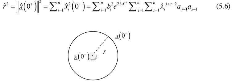
 0)

where

 

2

 

2 0

2 2 2 2

1 1

1 1 1 1

ˆ ˆ 0 n ˆ 0 n i n n j s

i i i j s

i i j s

r x  x  b e      a a

 

   

[image:22.595.137.513.556.689.2]

 

_



_

_{ }

(5.6)

Fig. 2: n-ball with centre x

 

0 and radius r

 

0 x 

S

r

(23)

22 Again, if the smooth approximation signal u t_( ) is applied, equation (4.6) should

be used; substitution into equation (5.6) shows that in this case we seek to maximise:

 

2 2





2 1

2 2 2 2 1

1 0 1ˆ 0 0 , .

i

n n

i i i

i i

r x  x  e    K    

 

 

  _   _

 



Next note that equation (4.5) gives:

 

0 1

1 1

ˆ 0 i n j

i i _j i j

x  b e   a

 



_

,

and hence

 

2 0

2 2 2

1 1 1 1

ˆ 0 i n n j s

i i _j _s i j s

x  b e      a a

   



_{ }

, i n

 (5.7)

Substituting, (5.7) into (5.6), gives

 

2 2





2 1

2 0

2 ₂ 1 2

1 1

1 1 1

0 n _i i i 0 , _i n n _ij s _j _s .

i j s

r x b e   K     a a

_

    

 

  

 

  _   _

 



 

(5.8)

Define the symmetric matrix









2 2

1 0

2 ₂ 1

( ) T ( ) , _i i i 0 , _i .

Q V D  V D diag b e   K   

_

 

 

  _   _

 

Note that due to the assumed controllability of ( , )A b (which implies that b_i 0,

in

) and the assumption that the eigenvalues of A are distinct (which implies that

det( )V 0), we have that ( )Q QT( ) 0. The two distance maximisation problems

now have the form

 

2

max r x 0 a QT ( ) a s t. . c_i a_i c_i, i n

     



and

 

2

ˆ ˆ

max r  x 0 a QT (0)a s t. . c_i a_i c_i, in,

(24)

23 which are Quadratic Programming optimization problems with “box” constraints. Since

the cost function ( ( )f a a QT ( ) a ) which is maximized is convex, the constrained

maximum is achieved in a vertex of a hyper-cube a_i c i_i, n.

Thus, we obtain







2



1 1

sgn sgn 0

j s

i aj as

   _ _

  for all j and k.

This can be easily derived if we assume that

 

1

sgna_j  1 j and

 

1 1

sgna_s  1 s ,

so we obtain

   

1 1

 

2

1 1

sgna_j_ sgna_s_  1 j 1 s  1 j s  .

So, the maximum distance is given by

 









2 2 2

1 0 ,

2 ₂ ₁

1 1

1 1 1 0 , .

iK i

n n n j s

i j s i

i j s

r  c c e     K   

 _

  _ _

    

 

 

 

 

  

 (5.9)

Finally, again if we assume that *



* *



*

, 0

t K t    , and



* *



,

K t  to beequal or greater to 3.90, we obtain

 

_*

 

2 2

1 1

1 1 1

0 n n n _i j s _j _s .

i j s

r x t x     c c

    

 

_{  }



(5.10)

The following numerical example illustrates some of the results of this section.

Example 5.2 Consider the (almost) zero state transition problem for the system defined in example 5.1 with x

 

0 0. Suppose that the following constraints are imposed on

the coefficients of the input signal

0 0 1

(25)

24 Subject to these constraints, the maximum distance from the zero state is:

 









 









2 2 2 2 1 1 1 2 ₂ 2 1 2 1 0 ,

2 2 2 2 ₂ ₁

1 1

1 1 1

2 1

0 ,

2 2 2 ₁

2

1 1 1 1

1 1

2 2

0 0 0

0 , .

0 , i i i i K j s

i j s i

i j s

K j s

j s

j s

x x x

c c e K

c                                        _ _            _   _                



  

 

_{}  





















2 2 2 2 2 2 1 0 ,

2 2 ₁

2

1 1 2

1 1

2 1 ₂ 2 ₂ 2 1 ₂ 2 ₂

1 0 1 1 1 1 1 1 2 0 1 2 2 1 1 2

1 1 1 1

2 2

2 2 2 2 2 2

1 2 0 0 1 1 2 2 0 1 1 1 2 1 1 1

0 , .

2 2

K j s

j s

s s s s

c e K

c c c c c c c c

c c c c c c

                            _                    _ _                 

 





In this example, c₀ 1, c₁2 and ₁ 2, ₂ 3. So, the maximum radius is given by

 



2 2





2 2





2 2



2 2

1 2 1 2 1 1 1 2

0 0 4 4 2 3 2 4 9 20 34

r x  x         

        

 .

Now, for the case that t*K t

r x t x        

6. Conclusions

In this paper, a novel methodology has been proposed for approximating the

distri-butional trajectory that transfers the state of a LTI differential system in (almost) zero

time by using an impulsive input. It has been shown that no loss of generality is

intro-duced if the impulsive input signal is chosen as a linear combination of the Dirac 

(26)

func-25 tion, and the resulting response of the system was analysed. The work has addressed the

following three distinct problems:

(i) We have determined the (unique) impulsive input signal (and its smooth

approxima-tion) which transfers the state of the system from the origin to an arbitrary point in state

space in zero (almost-zero) time, subject to appropriate controllability assumptions. To

simplify our presentation, the simplest set of assumptions has been selected (full system

controllability, single control input, distinct set of eigenvalues in the system matrix);

however, extension to the general case is straightforward at the expense of possible loss

of uniqueness and considerable additional complexity in the resulting mathematical

ex-pressions.

(ii) A Euclidean metric has been defined to quantify the approximation error in the

state-trajectories of the system resulting from substituting impulsive input signals by

smooth signals. The optimal choice of two parameters (time and volatility)

characteris-ing the family of all smooth approximatcharacteris-ing functions has been obtained, along with an

interesting probabilistic interpretation.

(iii) The solution of two state-space maximum-distance problems in the context of

(al-most) zero-time state-transition has been presented. These correspond to two different

types of constraints on the coefficients of the impulsive input signal and its smooth

ap-proximation, involving the Euclidian and infinity norms of the vector of coefficients.

Both problems are tractable and can be solved via an SVD and the solution of a

quad-ratic programming problem with box constraints, respectively.

Future work will attempt to: (i) extend the results of this paper to more general classes

of systems (e.g. descriptor, singular), (ii) investigate the numerical properties of

simu-lating impulsive trajectories and their smooth approximation, and (iii) develop

alterna-tive energy-based approximation techniques of impulsive behaviour especially in the

context of large-scale systems and model reduction.

Acknowledgment: Part of the present version of the paper has been presented in the 4th

(27)

26 2010, Ancona, Italy and in the Workshop “Advances in Mathematical Control Theory

and Applications", 19-20th of May 2011, Liverpool, UK. We are very grateful to Prof. Michael Malabre, Prof. Malcolm Smith, Prof. Jean-Jacques Loiseau, and Dr Efstathios

Antoniou for their helpful comments and remarks.

References

[1]. Bowen, J.M. (1994) Delta function terms arising from classical point source fields,

American Journal of Physics Vol. 62, pp. 511-515.

[2]. Boykin, T.B. (2003) Derivatives of the Dirac delta function by explicit construction

of sequences, American Journal of Physics Vol. 72, pp. 462-468.

[3]. Campbell, S.L. (1980) Singular systems of differential equations. I. Research Notes

in Mathematics 40. Pitman, Boston.

[4]. Campbell, S.L. (1982) Singular systems of differential equations. II. Research

Notes in Mathematics 61. Pitman, Boston.

[5]. Cobb, J.D. (1982) On the Solutions of Linear Differential Equations with Singular

Coefficients, Journal of Differential Equations Vol. 46, No. 3, pp. 310-323.

[6]. Cobb, J.D. (1983) Descriptor Variable Systems and Optimal State Regulation,

IEEE Transactions on Automatic Control Vol. 28, No. 5, pp. 601-611.

[7]. Cohen and Kirchner (1991), Approximating the Dirac distribution for Fourier

analysis, Journal of Computational Physic Vol. 93, pp. 312-324.

[8]. Estrada, R. and Kanwal, R.P. (2000) Singular integral equations, Birkhauser,

Bos-ton.

[9]. Gautshi, W. (1975), Optimally conditioned Vandermode matrices, Numerische