A computational method for the coupled solution of reaction-diffusion equations on evolving domains and manifolds : application to a model of cell migration and chemotaxis

Contents lists available atScienceDirect

Journal

of

Computational

Physics

www.elsevier.com/locate/jcp

A

computational

method

for

the

coupled

solution

of

reaction–diffusion

equations

on

evolving

domains

and

manifolds:

Application

to

a

model

of

cell

migration

and

chemotaxis

G. MacDonald

a

,

J.A. Mackenzie

a

,

∗

,

M. Nolan

a

,

R.H. Insall

b

a_{DepartmentofMathematicsandStatistics,UniversityofStrathclyde,Glasgow,G11XH,UnitedKingdom} b_{TheBeatsonInstituteforCancerResearch,GarscubeEstate,SwitchbackRoad,Glasgow,G611BD,UnitedKingdom}

a

r

t

i

c

l

e

i

n

f

o

a

b

s

t

r

a

c

t

Articlehistory: Received28March2015

Receivedinrevisedform16December2015 Accepted17December2015

Availableonline21December2015

Keywords: Reaction–diffusion Bulk–surfaceequations Cellmigration Chemotaxis

Evolvingfiniteelements ALEmethods Movingmeshmethods

Inthispaper,wedeviseamovingmeshfiniteelementmethodfortheapproximatesolution of coupled bulk–surface reaction–diffusion equations on an evolving two dimensional domain. Fundamental to the success of the method is the robust generation of bulk and surface meshes.For thispurpose, weuse anovel moving meshpartial differential equation(MMPDE)approach. Thedeveloped methodis appliedtomodel problemswith knownanalyticalsolutions;theseexperimentsindicatesecond-orderspatialandtemporal accuracy.Coupledbulk–surfaceproblemsoccurfrequentlyinmanyareas;inparticular,in the modelling of eukaryotic cell migrationand chemotaxis. We apply the methodto a model ofthe two-wayinteraction ofamigrating cell ina chemotacticfield,where the bulkregioncorrespondstotheextracellularregionandthesurfacetothecellmembrane. ©2016TheAuthors.PublishedbyElsevierInc.ThisisanopenaccessarticleundertheCC

BYlicense(http://creativecommons.org/licenses/by/4.0/).

1. Introduction

Coupled bulk–surface problems arise in many areas of engineering and the applied and natural sciences. Examples include crystal growth [29], interfacial fluid flows using soluble andinsoluble surfactants [7,27], proton diffusion along biologicalmembranes[34]andcellsignalling[47].

Ourmotivationforthedevelopment ofamethodforcoupledproblems onevolving domainscomes fromthe studyof eukaryoticcellmigrationandchemotaxis.Chemotaxis,inparticular,isessentialduringembryonicdevelopment,immunecell function, andcancermetastasis.Eukaryotic cells typically crawlby protruding pseudopods, whichare dynamic structures basedonactinfibres,atthefrontofthecell[26].Actinisaglobularproteinwhichspontaneouslypolymerises intolinear filaments that make up a large fractionofthe cell’s cytoskeleton. The key steplimitingactin polymerisation is the slow initiationofnewfilaments. Actinassembly canthereforebe stimulated by“nucleating factors” whichgeneratenewactin filaments.Inmostcells,actinfilamentsareconcentratedjustbeneaththecellularmembraneandcrosslinkedintoarelatively rigid cortex. Motor proteins such as myosin II bind to actin filaments in the cortex, crosslinking and contractingthem, causingcortical tensionand mechanicalresistance, whichtogether are key determinants ofcells’ overall behaviour. New actin polymerisation occurs betweenthecortex andthemembrane,givingrise to apressure pushingthe cellmembrane

*

Correspondingauthor.

E-mailaddress:[email protected](J.A. Mackenzie). http://dx.doi.org/10.1016/j.jcp.2015.12.038

outward atthe pseudopod; in other regions, cortical tension pulls along the remainder of thecell body. Together these processesleadtocellmovement.

In[40]wedevelopedapreliminarymodelofcellmigrationandchemotaxiswhereweonlyconsideredprocessestaking place on or closeto the cell membrane. The modelwas based ona systemof three reaction–diffusionequations posed onan evolvingcurveintwodimensions.Anevolvingsurface finiteelementmethodwasusedtoapproximatethesolution of the PDEs anda levelset method was usedto move the cell boundary. Themethod was later mademore robust and moreefficientbyreplacingthelevelsetmethodbyaparameterisedfiniteelementapproach[39].Themodelwasshownto predict manyaspects ofrealcellbehaviour such ascellpolarisation,persistentrandom walkmigration intheabsence of externalsignalsanddirectedmigrationinthepresenceofagradientinanexternalchemotacticfield[41].

The modelling of a numberof importantbiological processes however alsorequires the ability to solve model equa-tions in the extracellular and intracellular domains which are then coupled to equations posed on the cell membrane. It is also well appreciated that migrating cells have the ability to shape external chemotactic fields through the use of membrane-bound enzymes that degrade the ligand field andby the self-secretion of chemoattractants that allow signal relaytoneighbouringcells[50].Themodellingoftheseimportanteffectsrequirethecomputationalabilityofsolvepartial differentialequationsonevolvingbulk–surfacedomains.

Some previous computationalstudieslookingatbiologicalsignalling havebeencarriedoutassuming fixedcell bound-aries [36,30,42]. Methods have also been proposed to treat the deforming cell shape; for a recent review see [18]. For example, a phase-fieldapproach has been used to model the combined effect of intracellular actin-flow, cell adhesions and morphology on cell motility [48]. Normally phase-fieldmethods use isotropic stationarymeshes which makes their implementation relatively straightforward. However, as the phase-field is smoothed over a small width of size

ε

, the computational mesh needs to be fine enough to resolve this spatial scale which can make themethod computationally expensive unless some form of local mesh adaptation is used. Anotherwell known embedding method is the level set method(LSM)[44].Thisapproachusesanevolutionequationtomoveasigneddistancefunction;thezerolevelsetofthis function isthenidentifiedasthemovingcell boundary.LSMshavebeenusedsuccessfullyincell motilitymodels[49,54]. The disadvantageofLSMsistherequirementto maintainahighqualitysigneddistancefunctionwhichcan become diffi-cult ifthe evolvingcell morphologybecomes complicated. Bulk–surfacereaction–diffusionsystemsonstationarydomains havealsobeenaddressedusingasimplepoint cloudmethodin[31].An analysisofa finiteelementmethodforasteady state bulk–surfaceproblemispresentedin[13].Analysisandcomputationsofthediffusion-driveninstabilitypropertiesof coupledbulk–surfacereaction–diffusionsystemsonstationarydomainsispresentedin[32,33].

To approximatethe solutionofbulk–surface systemsof equationswe willuse an Arbitrary Lagrangian–Eulerian(ALE) approach. Traditionally,ALEmethodshave beenusedtosolve problemsonmoving domains usinga reformulationofthe original problemwith respect to an alternative reference frame rather than the standard fixed Eulerian frame. Forfluid dynamicsproblemsonecould decidetouseaLagrangian transformationtofollowthefluidflow. Moregenerallyhowever, there may be no obvious or preferred reference frame, and if the domain movesin time one may simply be satisfied witha transformationfromafixed stationarydomain

c ontothe physicallyevolvingdomain

(

t

).

TheALEformulation

was introduced forthis purpose and it has been used successfully to tackle a number of physical applications such as fluid–structure interaction systems (see [24,11]).In thispaperwe will usea conservative finiteelement ALEscheme.An advantage of thefinite element framework isit allows thenaturalincorporation of flux boundaryconditions linking the solution componentsin thebulk andsurface domains. Anotherpotential advantageof theALEapproach isthe abilityto accommodatearbitrarymeshmovementswhicharenotnecessarilyLagrangian.Thismayhelptherobustness,accuracyand efficiencyofthemethodwithfewerinstancesofremeshingbeingrequired.

Crucial tothesuccessofthefront-trackingapproachusedhereistherobust generationofcell body-fittedmeshes. For thispurposeweuseanadaptivemovingmeshprocedurebasedonthesolutionofamovingmeshpartialdifferential equa-tions (MMPDEs)[9,19,4,8,23]. Althoughadaptivemoving mesheshavebeenusedsuccessfullytosolve arange ofphysical problems[5,51,6],toourknowledgetheyhavenotbeenappliedtothegenerationofmeshesforcurvesevolvingaccording toa geometricevolutionlaw.Animportantcontributionofthispaperthereforeisthedevelopment ofan MMPDEmethod for the tangential motion of grid nodes along a curve which is moving with a specified normal velocity. The proposed method ismotivatedbythe approachofPanandWetton[45],whodevised afinite differenceschemeforthegeneration of mesheswhichequidistribute thearc-length betweengridnodes.The newmethodallows adegree ofcontrol over the generationofthesurfacemeshwhichisthenusedasknownboundaryconditionsforthegenerationofthebulkmesh.The additionalcontrol oftheboundarymeshalsoaddsconsiderablerobustness tothegridgenerationalgorithmleading tofar fewerinstancesfortheneedofglobalremeshingduetopoormeshquality.

[image:3.561.136.403.55.222.2]

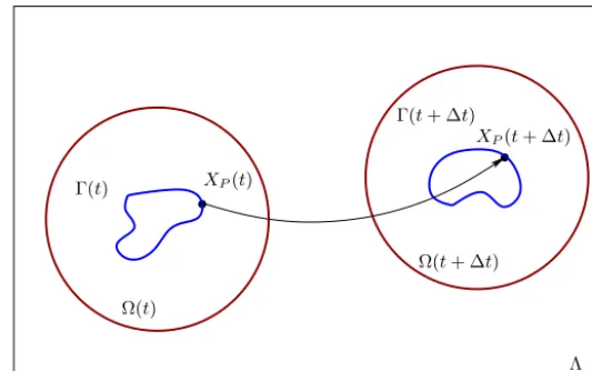
Fig. 1.Weconsiderthesimulationofamotilecellthroughafixedlabframeofreference.Thecellmembraneisdenotedby(t)andtheextracellular regionclosetothecellisdenotedby(t).Afteratimeintervalofsizet,thematerialpointlocatedat Xp(t)onthecellmembrane(t)evolvestothe newlocationXp(t+t).

2. Modelsystemequations

The physicallayout forthe cell migrationsimulations considered later is showninFig. 1.The cell membranewill be denoted by the evolving curve

(

t

).

The cell will be assumedto be moving through fixed lab frame ofreference

.

To improve computational efficiency, the governing equations for the extracellular region will only be computed over the time-dependenttwo-dimensionaldomain

(

t

),

whichiscentredonthecentroidofthecell.Wewillassumethatamaterial particle P locatedat Xp

(

t

)

on

(

t

)

has velocity X

˙

p

(

t

).

Therefore, we assume that thereexists a velocity field u so that

points on

(

t

)

evolve witha velocity field X

˙

p

(

t

)

=

u

(

Xp

(

t

),

t

).

Let n

=

(

n1

,

n2

)

denotethe unit outward normal to

(

t

)

andlet

N

(

t

)

beanyopensubset of

R

2 _containing

₍

_t

_).

_{Foranyfunction}

_ζ

_{whichisdifferentiablein}

_N

₍

_t

_),

_wedefinethe

tangentialgradienton

(

t

)

by

∇

ζ

= ∇ζ

−

(∇ζ

·

n

)

n,where

·

denotestheusual scalarproductand

∇ζ

denotestheusual gradienton

R

2.Foravectorfunction

ζ

=

(ζ

1

,

ζ

2

)

∈

R

2,thetangentialdivergenceisdefinedby

∇

·

ζ

= ∇ ·

ζ

−

2

i=1

(

∇

ζ

i

·

n

)

ni

.

TheLaplace–Beltramioperatoron

(

t

)

isdefinedasthetangentialdivergenceofthetangentialgradient

ζ

= ∇

·

(∇

ζ ).

Reaction–diffusionsystemsofthetype studiedinpatternformationgenerallyexcludecross-diffusionandareonly cou-pledbythereactionkineticsterms.Therefore,weconsiderthebehaviourofasinglechemicalspecieswithastraightforward generalisation toasystemofinteractingchemicals.Letusdefine

QT

= {

(

x

,

t

)

∈

R

3

:

x

∈

(

t

),

t

∈

(

0

,

T

]}

.

(1)

Application of Reynolds transport theorem to the equation formass conservation fora chemical C, which diffuses with constant D,undergoingreactionatarate f

(

c

),

gives

∂

c

∂

t

=

D

c

+

f

(

c

),

(

x

,

t

)

∈

QT

,

(2)

wherec

(

x

,

t

)

istheconcentrationatpositionx

∈

(

t

)

attimet.

WealsoconsidertheevolutionofachemicalspeciesCs,thatresidesontheboundary

(

t

).

ThebulkspeciesC willbe

coupledtoCsthroughthegenerallynonlinearfluxboundarycondition

Diffusive flux

−

D

∂

c

∂

n

(t)

+

Advective flux

(

u

·

n

)

c

|

_(t)

=

Rate of surface reaction

g

(

c

|

(t)

,

cs

),

(3)

where cs

(

x

,

t

)

denotes the concentration of Cs at the point x

∈

(

t

)

and n is the outward unit normal to

(

t

).

At the

In an analogousmanner tothe equationfor thebulk species,we will assumethat theboundary speciesevolvessuch that

∂

cs

∂

t

+ ∇

·

(

ucs

)

=

Ds

cs

+

g

(

c

|

(t)

,

cs

)

+

h

(

cs

),

(

x

,

t

)

∈

(

t

)

×

(

0

,

T

),

(4) where Dsistheboundarydiffusioncoefficient,h

(

cs

)

isasurfacereactionterm.

2.1. ALEreformulation

Forthereasonsmentionedearlier,whenthedomainismovingacommonframeofreferenceadoptedforcomputational purposes istheArbitraryLagrangian Eulerian(ALE) frame.Let

A

t beafamilyofbijectivemappings,whichateacht

∈

I

=

[

0,T

]

, map points ina referenceorcomputational configuration

c withcoordinates

ξ

=

(ξ,

η

),

topoints in thecurrent

physicalconfiguration

(

t

)

withcoordinatesx

=

(

x

,

y

),

sothat

A

t

:

c

⊂

R

2

→

(

t

)

⊂

R

2

,

x

(ξ

,

t

)

=

A

t

(ξ

).

(5)

Thecomputationalconfigurationcouldsimplybetheinitialphysicalconfiguration

(0).

Weleavethediscussion onhowto constructthemapping

A

t tosection4.

Foran arbitraryfunction g

:

QT

→

R

, definedon thefixed Eulerianframe,its temporalderivative intheALEframe is

definedas

∂

g

∂

t

ξ

:

QT

→

R

,

∂

g

∂

t

ξ

(

x

,

t

)

=

∂

g

ˆ

∂

t

(ξ,

t

),

ξ

=

A

−1

t

(

x

),

(6)

where g

ˆ

:

c

×

I

→

R

isthecorrespondingfunctionintheALEframe;thatisg

ˆ

(

ξ

,

t

)

=

g

(

x

(

ξ

,

t

),

t

)

=

g

(

A

t

(

ξ

),

t

).

Takingthe

timederivativeoftheALEmappingdefinestheALEvelocity w as

w

(

x

,

t

)

=

∂

x

∂

t

ξ

(

A

−_t1

(

x

),

t

).

(7)

It isimportantto note that theALEvelocity w on

(

t

)

will,in general,be differentfromthe materialvelocity u. When w

=

u theALEtransformationwillbe purelyLagrangianinnature. Torelate thetime derivativeswithrespect totheALE transformationtothematerialderivative,astandardapplicationofthechainrulegives

∂

c

∂

t

ξ

=

∂

c

∂

t

x

+

w

· ∇

c

.

(8)

Thereformulationof(2)intermsoftheALEreferenceframethereforetakestheform

∂

c

∂

t

ξ

−

w

· ∇

c

=

D

c

+

f

(

c

),

ξ

∈

c

.

(9)

Similarly,ontheboundarytheALEformulationof(4)takestheform

∂

cs

∂

t

ξ

+ ∇

·

(

ucs

)

−

w

· ∇

c

=

Ds

c

+

g

(

c

|

(t)

,

cs

)

+

h

(

cs

),

ξ

∈

∂

c

.

(10)

TheALEreformulatedequations(9)and(10)remaincoupledthroughthefluxboundarycondition(3).

2.2. AconservativeweakALEformulation

Toconstructaweakformulationof(9),weconsideraspaceofadmissibletestfunctionsdefinedonthereferencedomain made of functions v

ˆ

∈

H1

(

c

).

The ALEmapping then defines a set

H

((

t

))

of test functions on the domain

(

t

),

as

follows:

H

((

t

))

=

v

:

(

t

)

→

R

:

v

= ˆ

v

◦

A

_t−1

,

v

ˆ

∈

H1

(

c

)

,

t

∈

I

.

Aweakformulationof(9)canbeobtainedusingReynoldstransportformulawhichstatesthatif

ψ(

x

,

t

)

isafunctiondefined on

(

t

),

andVt

⊆

(

t

)

suchthat Vt

=

A

t

(

Vc

)

withVc

⊆

c,then

d dt

Vt

ψ (

x

,

t

)

dx

=

Vt

∂ψ

∂

t

ξ

+

ψ

∇ ·

w

dx

=

Vt

∂ψ

∂

t

x

+ ∇

ψ

·

w

+

ψ

∇ ·

w

dx

.

(11)

Asfunctionsv

ˆ

∈

H1

₍

d dt

(t) vdx

=

(t)

v

∇ ·

wdx (12)

and

d dt

(t)

v

ψ

dx

=

(t) v

∂ψ

∂

t

ξ

+

ψ

∇ ·

w

dx

.

(13)

Multiplying(9)byatestfunctionv

∈

H

((

t

)),

integratingover

(

t

)

andtheuseof(3),(12)and(13)givestheconservative weakform:findc suchthat

d dt

(t)

cvdx

−

(t)

(

∇ ·

(

wc

))

vdx

+

D

(t)

∇

c

· ∇

vdx

+

(t)

(

g

−

(

u

·

n

)

c

)

vds

=

(t)

f vdx

,

∀

v

∈

H

((

t

)).

(14)

Similarly,ontheboundarywehavetheconservativeweakformulation:findcssuchthat

d dt

(t)

csvsds

+

(t)

(

∇

·

((

u

−

w

)

cs

))

vsds

+

Ds

(t)

∇

cs

· ∇

vsds

=

(t)

(

g

+

h

)

vsds

,

∀

vs

∈

H

s

((

t

)),

(15)

where

H

s

((

t

))

=

vs

:

(

t

)

→

R

:

vs

= ˆ

vs

◦

A

t−1

,

v

ˆ

s

∈

H1

(

c

)

,

t

∈

I

,

isthespaceoftestfunctionon

(

t

).

3. Movingfiniteelementdiscretisation

3.1. Spatialsemi-discretisation

Wewillassumethat,foreacht

∈ [

0,T

]

,thephysicalandreferencedomains

(

t

)

and

careapproximatedbypolygonal

domains

h

(

t

)

and

c,h,respectively.Wewillassumethat

c,hiscoveredbyafixedtriangulation

T

h,cwithstraightedges,

sothat

c,h

= ∪

K∈Th,cK.The approximationoftheboundarydomain

h

(

t

)

ischosen tobesimplythe boundaryof

h

(

t

).

Thetotalnumberofelementsof

T

h,cwillbedenotedby N.Thetotalnumberofverticesof

T

h,c willbedenotedby

N

and

thenumberofverticesontheboundaryas

N

s.WedefinetheLagrangianfiniteelementspaceson

T

h,c as

L

1

₍

c,h

)

= {ˆ

vh

∈

H1

(

c,h

)

: ˆ

vh|K

∈

P1(

K

),

∀

K

∈

T

h,c}

,

L

1

0

(

c,h

)

= {ˆ

vh

∈

H1

(

c,h

)

: ˆ

vh|K

∈

L

1

(

c,h

)

: ˆ

vh

=

0

,

ξ

∈

c,h}

,

(16)

where

P

1

(

K

)

isthespaceoflinearpolynomialsonK.

Insection4wewilldescribeaprocedureforevolvingthenodalpositionsofthetriangulationcovering

h

(

t

).

Giventhe

locationofthemeshnodes,theALEmappingwillbeinterpolatedusingpiecewiselinearelementsgivingrisetoadiscrete mapping

A

h,t

∈

L

1

(

c,h

)

2oftheform

xh

(ξ

,

t

)

=

A

h,t

(ξ

)

=

N

i=1

xi

(

t

)

φ

ˆ

i

(ξ

),

(17)

wherexi

(

t

)

=

A

h,t

(

ξ

i

)

denotes thepositionofnode i attime t,and

φ

ˆ

i istheassociatednodalbasisfunction in

L

1

(

c,h

).

ThediscretisedALEvelocitythereforetakestheform

wh

(ξ

,

t

)

=

N

i=1

˙

xi

(

t

)

φ

ˆ

i

(ξ).

Let

T

h,t be the image of thereference triangulation

T

h,c underthe discrete ALE mapping

A

h,t. Since the mappingis

linear,each Kt whichistheimageofatriangle K

∈

T

h,c,isalsoatrianglewithstraightedges.UsingtheALEmapping,the

H

h

(

h

(

t

))

= {

vh

:

h

(

t

)

→

R

:

vh

= ˆ

vh

◦

A

−h,1t

,

v

ˆ

∈

L

1

(

c,h

)

}

.

The finiteelementspatial discretisationoftheconservativeALEformulation(14)thereforetakestheform:findch

(

t

)

∈

H

h

(

h

(

t

))

suchthat

d dt

h(t)

chvhdx

−

h(t)

(

∇ ·

(

whch

))

vhdx

+

D

h(t)

∇

ch

· ∇

vhdx

+

h(t)

(

g

−

(

u

·

n

)

ch

)

vhds

=

h(t)

f vhdx

,

∀

vh

∈

H

h

(

h

(

t

)).

(18)

Similarly,ontheboundary,wehavetheweakformulation:findcs,h

∈

H

s,h

(

h

(

t

))

suchthat

d dt

h(t)

cs,hvs,hds

+

h(t)

(

∇

·

((

u

−

wh

)

cs,h

))

vs,hds

+

Ds

h(t)

∇

cs,h

· ∇

hvs,hds

=

h(t)

(

g

+

h

)

vs,hds

,

∀

vs,h

∈

H

s,h

(

h

(

t

)).

(19)

Thefiniteelementapproximationofthebulkandsurfacespeciescanbeexpressedas

ch

(

x

,

t

)

=

N

j=1

cj

(

t

)φ

j

(

x

,

t

),

and cs,h

(

x

,

t

)

=

Ns

j=1

cs,j

(

t

)φ

s,j

(

x

,

t

),

where

{

φ

j

(

x

,

t

)

}

N_j=1 and

{

φ

s,j

(

x

,

t

)

}

N_j=s₁ arethe time-dependentbulk andsurface nodalbasis functions.If C

(

t

)

= {

cj

(

t

)

}

N_j=1

andCs

(

t

)

= {

cs,j

(

t

)

}

Nj=s1,wecanexpress(18)asthesystemofordinarydifferentialequations

d

dt

(

M

(

t

)

C

(

t

))

+ [

K

(

t

)

+

A

(

t

,

wh

(

t

))

−

B

(

t

,

wh

(

t

))

]

C

(

t

)

+

D

(

C

(

t

),

Cs

(

t

))

=

F

(

C

(

t

)),

(20) where

[

M

(

t

)

]i j

=

h(t)

φ

i

(

t

)φ

j

(

t

)

dx

isthe(time-dependent)massmatrix,while

[

K

(

t

)

]i j

=

D

h(t)

(

∇

φ

j

(

t

)

· ∇

φ

i

(

t

))

dx

,

[

A

(

t

,

wh

(

t

))

]i j

=

h(t)

[

(

u

−

wh

)

·

n

]

φ

i

(

t

)φ

j

(

t

)

ds

,

[

B

(

t

,

wh

(

t

))

]i j

= −

h(t)

[

wh

· ∇

φ

i

(

t

)

]

φ

j

(

t

)

dx

,

[

D

(

C

(

t

),

Cs

(

t

))

]i

=

h(t)

[

g

(

ch

(

t

),

cs,h

(

t

))

−

(

u

·

n

)

ch

(

t

)

]

φ

i

(

t

)

ds

,

andtheloadvector

[

F

(

C

(

t

))

]i

=

h(t)

f

(

ch

(

t

))φ

i

(

t

)

dx

.

Note thatthevector D willbesparse asonlythosevaluesofi correspondingto boundaryverticeswillbe non-zero.The spatialdiscretisationoftheboundaryequation(19)resultsinasystemofODEs

d

[

Ms

(

t

)

]i j

=

h(t)

φ

s,i

(

t

)φ

s,j

(

t

)

ds

,

[

Ks

(

t

)

]i j

=

Ds

(t)

(

∇

φ

s,j

(

t

)

· ∇

φ

s,i

(

t

))

ds

,

[

As

(

t

,

wh

(

t

))

]i j

=

h(t)

[∇

·

(

u

−

wh

)

]

φ

s,i

(

t

)φ

s,j

(

t

)

+ [

(

u

−

wh

)

· ∇

φ

s,j

(

t

)

]

φ

s,i

(

t

)

ds

,

[

H

(

Cs

(

t

))

]i

=

h(t)

h

(

cs,h

(

t

))φ

s,i

(

t

)

ds

,

andDsaretheappropriatelyreorderednon-zeroelementsof D.

3.2. Temporalintegration

Toobtainatemporaldiscretisationof(20)and(21)wesubdivide

[

0,T

]

into Nt equaltimeintervalsofsize

t

=

T

/

Nt

anddenotetn

=

n

t,n

=

0,1,

. . . ,

Nt.We willdiscretise theALEmappingusinglinearinterpolation betweentimelevels.

Thatiswewilldefine

A

h,t

(ξ

,

t

)

=

t

−

tn

t

A

h,tn+1

(ξ

)

+

tn+1

−

t

t

A

h,tn

(ξ),

t

∈ [

tn

,

tn+1), (22)

where

A

h,t isthepiecewiselinearmapattimet.Themeshvelocityisthereforepiecewiseconstantintimeandisgivenby

wn_h+_,1_t

(ξ

)

=

A

h,tn+1

−

A

h,tn

t

,

t

∈ [

t

n

_,

_tn+1

_),

wn_h+_,1_t

(

x

,

t

)

=

wn_h+_,1_t

(ξ

)

◦

A

−_h,1_t

(

x

).

(23)

Thetemporaldiscretisationofthecoupledsystems(20)and(21)isobtainedusingamodifiedCrank–Nicolsonsemi-implicit approach. We first predict the boundary solution C

˜

_sn+1 using a semi-implicit backward Euler method, where the linear diffusion and mesh movement terms are treated implicitly, and the nonlinear reaction and coupling terms are treated explicitly.Thepredictedboundarysolutionthereforesatisfiesthelinearsystem

[

Mn_s+1

+

t

(

K_sn+1

+

A_sn+1

)

] ˜

Cn_s+1

=

Mn_sCn_s

+

t

[

Ds

(

Cn

,

Cns

)

+

H

(

Cns

)

]

.

(24)

ThebulkapproximationisthenupdatedusingaCrank–Nicolsonstep

[

Mn+1

+

1₂

t

(

Kn+1

+

An+1

+

Bn+1

)

]

Cn+1

= [

Mn

−

1₂

t

(

Kn

+

An

+

Bn

)

]

Cn

+

1₂

t

[

F

(

Cn+1

)

+

F

(

Cn

)

−

D

(

Cn+1

,

C

˜

_sn+1

)

−

D

(

Cn

,

Cn_s

)

]

.

(25)

Thenonlinearsystem(25)issolvedusingNewtoniteration.Finally,toensurethattheboundarysolutionissecond-orderin time,weperformaCrank–Nicolsoncorrectionstep

[

Mn_s+1

+

1₂

t

(

K_sn+1

+

An_s+1

)

]

Cn_s+1

= [

Mn_s

−

1₂

t

(

Kn_s

+

An_s

)

]

Cn_s

+

1₂

t

[

Ds

(

Cn+1

,

C

˜

n+1

s

)

+

Ds

(

Cn

,

Cns

)

+

H

(

C

˜

n+1

s

)

+

H

(

Cns

)

]

.

(26)

Notethatthiscorrection steponlyrequiresthesolutionofalinearsystemofequationsevenifthereactiontermsonthe surface, g andh arenonlinear.The linearsystemsarisingaboveare solvedusingtheiterativemethodBiCGSTAB[52] and anincompleteLU(ILU)factorisation asapreconditioner.

Forthecellmigrationapplicationconsideredlater,wenotethat thediffusivetime scalesintheextracellularregionare oftenmuchshorterthanthetimescaleassociatedwithcellmigration.Asthetimeintegrationschemeaboveisfullyimplicit inthediffusivetermsitisthereforerobusttothechoiceofthetimestepfortheseapplications.

3.3. Amodelbulk–surfaceproblemonastationarydomain

∂

c

∂

t

=

c

,

x

∈

(27)

∂

cs

∂

t

=

cs

+

c

−

cs

,

x

∈

,

(28)

−

∂

c

∂

n

=

c

−

cs

,

x

∈

,

(29)

where

istheunitcircle.

Thisproblemcanbetackledanalyticallyusingpolarcoordinatesx

=

rcos

θ,

y

=

rsin

θ

sothat

∂

c

∂

t

=

∂

2c

∂

r2

+

1 r

∂

c

∂

r

+

1 r2

∂

2c

∂θ

2

,

x

∈

∂

cs

∂

t

=

∂

2cs

∂θ

2

+

c

|r

=1

−

cs

,

x

∈

,

and

−

∂

c

∂

r

r=1

=

c

|r

₌1

−

cs

.

SimilartoNovaketal.[43],welookforasolutionintheform

cs

(θ,

t

)

=

Ae−k 2_t

cos

θ,

and

c

(

r

, θ,

t

)

=

ρ

(

r

)

cs

(θ,

t

).

Thefollowingexactsolutionhasbeenusedtotesttheconvergenceofthefiniteelementdiscretisation:

c

(

r

, θ,

t

)

=

J1(rk

)

e−k2tcos

θ

and

cs

(θ,

t

)

=

J1(k

)

2

−

k2e− k2t_cos

_θ,

where J1isthefirst-orderBesselfunctionofthefirstkindandk

=

1.177706027.

Fig. 2 showsthe computedapproximatesolutions inthebulk domainandon thedomainboundaryusingan isotropic mesh withmaximal celldiameterh

=

0.1 anda timestep

t

=

2

×

10−4.We canseethatthemethodperforms wellfor these values ofthe discretisation parameters. Totest the spatial rateof convergence ofthe algorithm, simulations were performed ona sequenceofincreasingly refined isotropicmeshes. Toensure that theerrorwas dominated byits spatial component, asufficiently smalltime stepof

t

=

10−3 was used.Fig. 3(a)showsthemaximumerroroverall gridnodes for boththe bulk andsurface numericalsolutions andwe can seethat both convergeat therateof O

(

h2

_),

_asexpected.

To investigatethetemporal rateofconverge, simulations were performedusinga finemesh withN

=

150,000 elements andvarious time steps.Wecan seefromFig. 3(b),that thethree-stepsolutionprocedure (24)–(26)furnishes approxima-tions whicharesecond-orderaccurate intime.Notethatifthesurfacesolutioncorrectionstep(26)wereomittedthen,as expected,theresultingapproximationswereonlytemporallyfirst-orderaccurate.

4. PracticalevaluationofALEmapping

For the ALEmapping to be useful, it must satisfy a numberof properties.First, it must be inexpensive to construct, relative to thecost ofsolving thephysicalproblem. Second, theresulting meshescovering

(

t

)

mustbe ofgoodquality in thesense thatmeshelements are adaptedto salientfeaturessuch atsteepboundary orinteriorlayersinthe physical solution.Finally,themeshesmustevolvesmoothlyintimetoavoidtheneedtousesmalltimestepstomaintainnumerical stability.

4.1. Bulkdomainmeshgeneration

To avoid potential mesh crossings or foldings, we derive a suitable evolution equation forthe inverse ALE mapping

A

−1

t

(

x

)

=

ξ

(

x

,

t

)

ratherthan

A

t

(

ξ

)

=

x

(

ξ

,

t

)

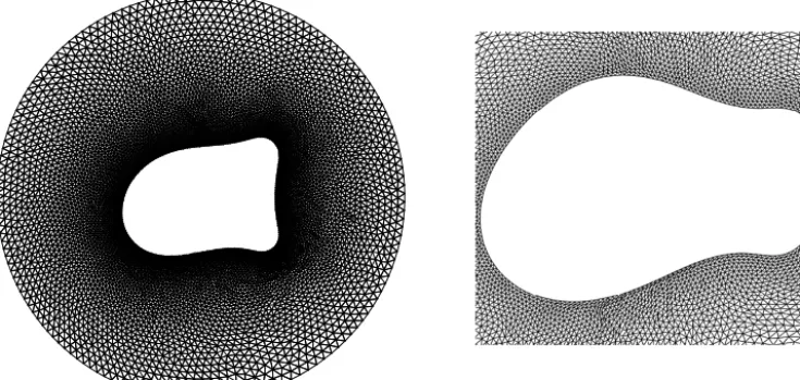
(see,forexample,thediscussionin[12]).As showninFig. 4,a mesh

T

h,t on

h

(

t

)

canthenbe generatedasthepreimageofafixedmesh

T

h,c on

c,h.Asintroducedin[22],wechoosethemapping

ξ

(

x

)

correspondingtoafixedvalueoft inordertominimisethefunctional

I

[

ξ

] =

1

2

t

Fig. 2.Numericalsolutionofcoupledmodelproblem(27)–(29)onastationaryunitcircle.(a)Approximatebulksolutionch(x)att=1.(b)Approximate solutioncs,h(θ )ontheboundarycomparedtotheexactsolution.

Fig. 3.Second-order convergence of the maximum nodal error as (a)h→0 and (b)t→0 for a coupled model problem on a unit circle.

Fig. 4.A moving mesh covering(t)is the image of a fixed mesh on a reference domaincthrough a time-dependent ALE mappingAt(ξ)=x(ξ,t).

where G is a 2

×

2 symmetric positive definite matrix referred to as a monitor matrix and

∇

is the gradient operator with respect to x. It can be shown that the functional (30) is coercive and uniformly convex andhence has a unique minimiser[23].

Rather than directly attempt to minimise (30), a more robust procedure is to evolve the mapping according to the modifiedgradientflowequations

∂ξ

∂

t

=

P

τ

∇ ·

(

G

−1

_∇

_{ξ ),}

_and

∂

η

∂

t

=

P

τ

∇ ·

(

G

Here,

τ

>

0 isauser-specifiedtemporalsmoothingparameterwhichaffectsthetemporalscaleoverwhichthemeshadapts and P is a positivefunction of

(

x

,

t

),

chosen such that the meshmovement hasa spatially uniformtime scale [19].The gradient flowstructureof(31)ensures thatthe meshevolvessmoothly intime andimproves robustnessinthechoice of theinitialmesh.

The selection of an appropriate monitor matrix is crucial to the success of mesh adaptation. In this paper, we will considerthemonitormatrixproposedbyWinslow[53]

G

=

M 0 0 M

,

(32)

whereM

(

x

,

t

)

isapositiveweightfunctioncalledamonitorfunction.Asuitablemonitorfunctionisessentialtothesuccessof adaptivemovingmeshmethods.ThemonitorfunctionshouldbetayloredtothetypeofPDEbeingsolvedandthenumerical method being used. Monitor functions based on interpolation estimates, a posteriori error estimates and adaptation to solutionfeatureshaveallbeenproposed[3,8,23].Ifnosuchestimateexiststhenthemonitorfunctioncouldbeanysmooth function designed to adaptthe mesh towards importantsolution features such moving interfacesor boundaries(see for example[5]).

In practice,we interchangetherolesofthedependent andindependentvariables in(31),sinceit’sthelocation ofthe physicalmeshpoints

{

xi

(

t

)

}

Ni=1 thatdefinestheALEmap.WithaWinslow-typemonitormatrix(32)theresultingMMPDEs

taketheform

τ

∂

x

∂

t

=

P

(

axξ ξ

+

bxξη

+

cxηη

+

dxξ

+

exη

),

(ξ,

η

)

∈

c

,

(33) where

a

=

1 M

x2 η

+

y2η

J2

,

b

= −

2 M

(

xξxη

+

yξyη

)

J2

,

c

=

1 M

x2_ξ

+

y2_ξ

J2

,

d

=

1

(

M J

)

2

[

Mξ

(

x 2

η

+

y2η

)

−

Mη

(

xξxη

+

yξyη

)

]

,

e

=

1

(

M J

)

2

−

Mξ

(

xξxη

+

yξyη

)

+

Mη

(

x2ξ

+

y2ξ

)

,

and J

=

xξyη

−

xηyξ istheJacobianoftheALEmapping.Tocompletethespecificationofthecoordinatetransformation,the MMPDEmustbesupplementedbyinitialandboundaryconditions.Inalltheapplicationsdescribedlater,thecomputational domain

c,h

=

h

(0),

andthe initialmeshover thephysicaldomainisobtainedusingtheMatlab toolboxDistmesh [46].

To allow the mesh points to move along the boundary

h

(

t

),

they are obtained using a one-dimensional moving mesh

approach outlined in section 4.2. Once the boundary nodes have been evolved over one time step, they then become Dirichletconditionscompletingthespecificationfor(33).

Thenumericalsolutionof(33)requiresspatialandtemporaldiscretisation.Inspace,wediscretise usingstandardlinear Galerkin finite elements. In the time direction, we use a backward Euler integration scheme to update the solution at

t

=

tn+1_{, andto avoidsolving nonlinear algebraic systems,we evaluate the coefficientsa}

_,

_c

_,

_{. . . ,}

_{e at thetime t}

₌

_tn_{. We}

thereforeseekxn_h+1

∈

(

L

1

₍

c,h

))

2suchthat

τ

c,h

xn_h+1

−

xn_h

t

·

v

ˆ

hd

ξ

+

c,h

(

xn_h+1

)

ξ

·

(

anv

ˆ

h

)

ξ

+

(

xnh+1

)

η

·

(

cnv

ˆ

h

)

η

+

1

2

[

(

x

n+1

h

)

ξ

·

(

bnv

ˆ

h

)

η

+

(

xnh+1

)

η

·

(

bnv

ˆ

h

)

ξ

] − [

dn

(

xnh+1

)

ξ

+

en

(

xnh+1

)

η

] ·

v

ˆ

h

d

ξ

=

0

,

(34)

forall v

ˆ

h

∈

(

L

10

(

c,h

))

2.TheresultinglinearsystemsareagainsolvedusingtheiterativemethodBiCGSTABandan

incom-plete LU(ILU) factorisation asa preconditioner. Ananalysisofthe performance ofthisiterativesolverfor thediscretised MMPDEequationscanbefoundin[4].

4.2. Boundarymeshgeneration

Weconsidertheclassofboundarymovementsgivenbythefollowingevolutionlawforthenormalvelocity

V

(

x

,

t

)

=

ακ

+

β,

x

∈

(

t

),

(35)

where

κ

isthecurvature.Withinthecontextofbiologicalcellapplications,thefunctions

α

and

β

couldmodelthephysical forcesexertedonthemembranebycorticaltension,andprotrusionscausedbyactinpolymerisation,respectively.

Weconsiderthesolutionof(35)usingaLagrangianapproach,wherethemainideaistorepresenttheflowofcurvesby thepositionvectorxwhichisthesolutionofthegeometricevolutionequation

˙

wherenandt areunitnormalandtangentvectors,respectively.Notethatthepresenceofthetangentialvelocity

B

hasno effectontheshapeoftheevolvingcurvebutitiswellknownthattheincorporationofasuitablychosennon-zerovalueof

B

canavoidthemajordrawbackoftheLagrangianapproachwhichisthepossibilitythat gridpointsmerge,resultingina lossofstabilityandaccuracy[2,1,37].

An embeddedregular plane curve

canbe parameterised by thesmooth function x

:

S1

_→

_R

2_,i.e.

₌

_Image(x

₎

_:=

{

x

(

σ

),

σ

∈

S1

_}

_{.Takingintoaccount theperiodic boundaryconditionsat}

_σ

₌

_{0,1,weshall hereafteridentify S}1 _withthe

interval

[

0,1

]

.Theunitarc-lengthparameterisationwillbedenotedby sanditcanbeshownthatxs

=

t andxss

=

κ

n.The

arc-lengthofthecurvefromthepointx

(

σ0

)

tox

(

σ

)

isgivenby

s

(

σ

)

=

σ

σ0

x2

σ

+

y2σd

σ

=

σ

σ0

xσ

d

σ

,

where

·

denotesthel2-norm.Usingthechainrule

x_σ

=

xs

ds

d

σ

=

xsxσ

(37)

anddifferentiationof(37)leadstotherelation

xσ σ

=

xssxσ

2

+

xsxσ

s

xσ

.

(38)

Multiplyingthrough (38)by n,we getanexpressionfor

κ

andhenceintermsoftheparameterisation

σ

,we canexpress thenormalvelocityas

V

= ˙

x

·

n

=

α

x_{σ σ}

·

n

xσ

2

+

β.

(39)

Controlofthe meshspacinginthe tangential directioncanbe achievedby ensuringthat aweighted arc-length between gridnodesisconstant.Thatis,ifM

(

x

,

t

)

>

0 isapositivemonitorfunction,thenweset

M ds

d

σ

=

constant andhence

M ds

d

σ

σ

=

(

M

xσ

)

σ

=

0

.

(40)

Thedifferential-algebraicsystem(39)and(40)could,intheory,beusedtoevolvetheboundary

(

t

);

thecase

α

=

1,

β

=

0 andM

=

1,whichaimstoconstructauniformarc-lengthparameterisation,isexactlytheequationsystemusedbyPanand Wetton[45].In[39] weusedtheparameterisedfiniteelementmethod(PFEM)[2]to evolvetheapproximationofacurve describing anevolving cell membrane.Thismethodintroduces an intrinsictangential velocity

B

suchthat thearc-length betweengrid nodesis equidistributed. When using thePFEM togenerate boundarynode displacements,which are then used as boundary data formeshes covering bulk regions, we have found that the lack of control of the PFEM intrinsic tangentialvelocitycanleadtopoorqualitybulkmeshes whichrequirefrequentremeshing.Experiencewiththegeneration of adaptive moving meshes suggestshowever that the introduction of an evolution equation for the tangential velocity, drivenby themeshequidistributioncondition (40),can significantlyimprovestabilityandrobustness [21,20,3].Therefore, weconsiderthetangentialvelocityequation

B

= ˙

x

·

t

=

P

τ

(

M

xσ

)

σ

,

(41)

where,asbefore,

τ

andP areatemporalsmoothingparameterandspatialbalancingoperator,respectively. Theproposed procedurethereforeinvolvesthesimultaneoussolutionof(39)and(41).

Forsimplicity,wediscretise(39)and(41)usingafinitedifferencemethod.Theevolvingcurveattimetn _{isrepresented}

bythediscreteplanepoints xn_i,i

=

1,

. . . ,

N

s.Thelinearapproximationofthecurveisthereforegivenbythepolygonwith

verticesxn_i,i

=

1,

. . . ,

N

s.Duetotheperiodicityconditions,we alsousetheadditionalvaluesxn₋₁

=

xn_Ns−1, xn₀

=

xn_Ns and

xn_N

s+1

=

x n

1.Weuseauniformdiscretisationoftheparameterisationinterval

σ

∈ [

0,1

]

withstepsize

σ

=

1/

N

s.Weuse

centralfinitedifferencestoapproximatethespatialderivativesin(39)andafirst-orderfullyimplicittemporaldiscretisation. Thisleads to anonlinear systemwhichis solvedusing Picarditeration. Letx[n,m] _{denotethe approximationof x attime} leveltn _{anditerationlevelm,thenforthenormalvelocityequationswehavethelinearsystem}

[−

μ

[_in+1,m]x_i[₋n+₁1,m+1]

+

(

1

+

2

μ

[_in+1,m]

)

x_i[n+1,m+1]

−

μ

_i[n+1,m]x[_in₊+₁1,m+1]

] ·

n[_in+1,m]

fori

=

1,

. . . ,

N

s,where

μ

[in,m]

=

4tαi

/(

x[in+,m1]

−

x[ n,m]

i−1

2

).

Weapproximatetheunittangentvector

tn_i

=

x

n

i+1

−

xni−1

xn

i+1

−

xni−1

=

(

tn₁

,

tn₂

),

andhencewesetnn

i

=

(

tn2

,

−

tn1

).

Usingasimilardiscretisationofthetangentialvelocityequation(41)wehave

[−

ν

_inx_i[n₋+₁1,m+1]

+

(

1

+

2

ν

_in

)

x[_in+1,m+1]

−

ν

_inx_i[₊n+₁1,m+1]

] ·

t[_in+1,m]

=

xn_i

·

t_i[n+1,m]

+

t Pi 4

τ

(

σ

)

2

(

M

n

i+1

−

Mni−1

)(

x[ n+1,m]

i+1

−

x[ n+1,m]

i−1

),

(43)

fori

=

1,

. . . ,

N

s,where

ν

n_i

=

t Mn_iPi

/(

τ

(

σ

)

2

).

Thecoupledsetof2

N

sequations(42)and(43)aresolvedforx[n+1,m+1]

andthePicarditerationisstoppedwhen

x[n+1,m+1]

−

x[n+1,m]

<

TOL

.

Thelastiterationisthenusedastheapproximationxn+1.

4.3. Example

To demonstrate the capability of the proposed adaptive grid generation procedures, we consider the evolution ofan ellipseundermeancurvatureflowwhere

V

= −

ακ

,andsimultaneouslywerequirethebulkandsurfacemeshesevolveto resolvethetravellingwaveprofile

u

(

x

,

y

,

t

)

=

1

2

1

+

tanh

x

+

t

−

0

.

7 0

.

6

.

Therearemanypossiblechoicesforthemonitorfunctionbutforillustrativepurposeswewillset

M

(

x

,

y

,

t

)

=

1

+

sech2

x

+

t

−

0

.

7 0

.

6

.

The monitorfunctiontakesits maximumvalue atthecentreofthetravellingwaveanddecreasessmoothly toanon-zero constant value farfromthefront. Theresultingadapted meshshould thereforebe clusteredaroundthewave butalmost uniform inthe flatregions. The initial physicaldomain consistsofthe region exterior to theellipse 4x2

+

16y2

=

1 and interiortoaunitcircularfar-fieldboundary;thefixedcomputationaldomain

cischosentobetheinitialphysicaldomain.

The computational mesh is obtainedusing the Matlab toolbox Distmesh [46] andhas N

=

9832 elements and

N

s

=

98

vertices on the boundary of the ellipse.The simulations are performed over the time interval t

∈ [

0,7

×

10−2

_]

_{using a}

constant time step

t

=

10−3_{.The coefficientofthe normalvelocityofthe evolvingcurve is}

_α

₌

_{0.75,andthe temporal}

smoothingparametersinthemovingmeshPDEsareboth

τ

=

10−4.Thecomputedmeshesatfourrepresentativetimesare showninFig. 5.We canseethat theinitialmesh isadaptedtowards thewavefront whichiscentredto therightofthe ellipseatx

=

0.7.Initiallytheboundarymeshpointsaredistributedtoequidistributethearc-lengthasthemonitorfunction

M

≈

1 alongtheellipse.Att

=

0.02 and t

=

0.04,we canseethat thebulkmesheshavemovedtofollowthewavefront; theboundarymesheshavealsoadaptedcorrectlyinthetangentialdirectionandevolvedinthenormaldirectionaccording tothecurvatureoftheboundary.Finally,att

=

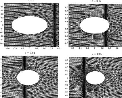
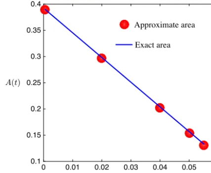
0.05,thewavefronthaspassedbytheinnercurveandtheboundarymesh relaxesbacktoequidistributethearc-lengthbetweenmeshpoints.Fig. 6showstheadapted boundarymeshes;forclarity, atthetwotimeswhenthewavefrontintersectstheboundary,wehaveindicateditslocationbyaverticaldashedline.We can seethatatthesetimestheboundarymeshhasadaptedwell tothewave frontandattheother twotimesthemesh equidistributesthearc-lengthoftheevolving curve. Totest theaccuracyofthecomputedmoving boundary,Fig. 7shows theevolutionoftheexactandapproximateareaenclosedbytheclosedcurve;theexactareaformeancurvatureflowtakes theform A

(

t

)

=

A

(0)

−

2

π αt

.Wecanseethattheapproximateareadecreaseslinearlyintime,andatthetimesindicated itagreeswellwiththeexactarea.

5. Thecompletealgorithm

We now describe thecomplete algorithm implementing the ALE–FEMscheme andthe generation of the surface and bulk meshes. At time t

=

tn _{we assume we havea mesh}

_T

h,tn andthe finiteelement approximations cn h andc

n s,h of the

bulkandsurfacespecies,respectively.Thefollowingstepsarethencarriedouttoadvancethemeshandthefiniteelement approximations.

1.Updatethephysicalmesh

(a) Usingcn_s,h,calculatethenormalvelocityof

givenby(35).

[image:13.561.61.485.59.400.2]

Fig. 5.Adaptivebulkmeshesfor atime-dependentdomainwheretheinnerboundary evolvesbymeancurvatureflow.Themeshesareadapted toa travellingwaveprofilemovingacrossthedomainfromrighttoleft.

[image:13.561.140.403.477.659.2]

[image:14.561.166.380.56.231.2]

Fig. 7.Comparisonoftheevolutionoftheexactandcomputedareaenclosedbyaclosedcurveundermeancurvatureflowatt=0,0.02,0.04,0.05 and t=0.055.

(c) Usingthebulkapproximationcn_h,determinethemeshadaptationmonitorfunctionM.

(d) UsingtheupdatedboundarypointsasfixedDirichletdata,updatetheinteriormeshpointsbysolving(34). (e) Testformeshquality.Ifthemeshisfinethengoto2.Ifnotthenre-gridandinterpolatethesolutionsontothenew

meshandre-dothetimestep.

2.Updatethefiniteelementsolutionsinthebulkandthesurface

(a) Usethemeshes

T

_h,tn+1 and

T

_h,tn todefinethediscreteALEvelocityw_h.

(b) Updatethesolutionscn_s,+_h1 andcn_h+1bysolving(24)–(26).

Todeterminethequalityofthebulkmesheswemeasuretheminimumangleoverallofthetrianglesanddecidetoremesh whenthisisbelowagiventolerance.Thenewmeshcoveringthephysicaldomainisthenusedasthefixedcomputational mesh.Thebulkandboundarysolutionsarethenlinearlyinterpolatedontothenewmeshtoallowfurthertimeintegration.

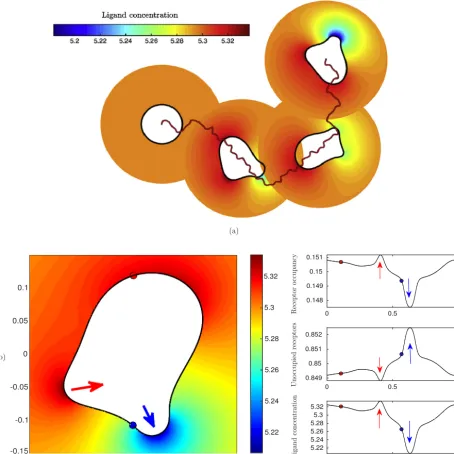
6. Cellmigrationandchemotaxis

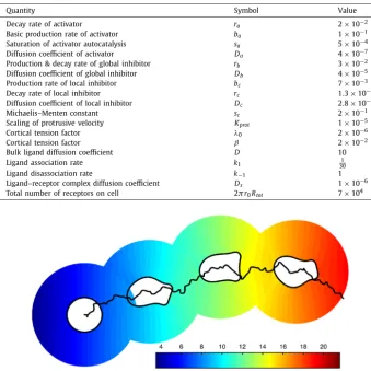
Wenowconsidertheapplicationofthedevelopedalgorithmtothecomputationalmodellingofeukaryoticcellmigration andchemotaxis.In[40,41]wedevelopeda“pseudopod-centered”[25]modelbasedonasystemofreaction–diffusion equa-tionsthatgivesrisetoasuitablespatiotemporalactivatorprofilethatcanbeusedforthegenerationofpseudopodswithout the needfora drivingexternal signal.The followingsetofequationswas derived fromawell-establisheddiscrete model developed byMeinhardt [35](Mmodel). Themodeldescribesthedynamic interactionbetweenamembrane-bound local autocatalytic activatora,a rapidlydistributed globalinhibitorb anda localinhibitor c. Assumingthat the cell boundary

(

t

)

moveswithvelocityu,thenforx

∈

(

t

)

theequationstaketheform

∂

a

∂

t

+ ∇

·

(

ua

)

=

Da

a

+

s

(

a2

/

b

+

ba

)

(

sc

+

c

)(

1

+

saa2

)

−

raa

,

(44)

∂

b

∂

t

+ ∇

·

(

ub

)

=

Db

b

−

rbb

+

rb

|

(

t

)

|

(t)

adx

,

(45)

∂

c

∂

t

+ ∇

·

(

uc

)

=

Dc

c

+

bca

−

rcc

.

(46)

Here,ra

,

rb andrc denotedecayratesofthelocalactivator,globalinhibitorandlocalinhibitor,respectively.The

correspond-ing diffusioncoefficients are Da

,

Db and Dc. In thenonlinear reaction term in theactivator equation, sa is a saturation

coefficient,sc isaMichaelis–Mentenconstantandbaisabasalproductionrateoftheactivator.Theconstantbc determines