A search algorithm for global optimisation

S. Chen1_{, X.X. Wang}2_{, and C.J. Harris}1

1 _{School of Electronics and Computer Science,}

University of Southampton, Southampton SO17 1BJ, U.K 2 _{Neural Computing Research Group, Aston University,}

Birmingham B4 7ET, U.K

Abstract. This paper investigates a global search optimisation technique, re-ferred to as the repeated weighted boosting search. The proposed optimisation algorithm is extremely simple and easy to implement. Heuristic explanation is given for the global search capability of this technique. Comparison is made with the two better known and widely used global search techniques, known as the genetic algorithm and adaptive simulated annealing. The effectiveness of the pro-posed algorithm as a global optimiser is investigated through several examples.

1

Introduction

Evolutionary and natural computation has always provided inspirations for global search optimisation techniques. Indeed, two of the best-known global optimisation algo-rithms are the genetic algorithm (GA) [1]-[3] and adaptive simulated annealing (ASA) [4]-[6]. The GA and ASA belong to a class of guided random search methods. The un-derlying mechanisms for guiding optimisation search process are, however, very differ-ent for the two methods. The GA is population based, and evolves a solution population according to the principles of the evolution of species in nature. The ASA by contrast evolves a single solution in the parameter space with certain guiding principles that imitate the random behaviour of molecules during the annealing process. It adopts a re-annealing scheme to speed up the search process and to make the optimisation process robust.

We experiment with a guided random search algorithm, which we refer to as the repeated weighted boosting search (RWBS). This algorithm is remarkably simple, re-quiring a minimum software programming effort and algorithmic tuning, in compari-son with the GA or ASA. The basic process evolves a population of initially randomly chosen solutions by performing a convex combination of the potential solutions and replacing the worst member of the population with it until the process converges. The weightings used in the convex combination are adapted to reflect the “goodness” of corresponding potential solutions using the idea from boosting [7]-[9]. The process is repeated a number of “generations” to improve the probability of finding a global op-timal solution. An elitist strategy is adopted by retaining the best solution found in the current generation in the initial population of the next generation. Several examples are included to demonstrate the effectiveness of this RWBS algorithm as a global optimi-sation tool and to compare it with the GA and ASA in terms of convergence speed.

L. Wang, K. Chen, and Y.S. Ong (Eds.): ICNC 2005, LNCS 3611, pp. 1122–1130, 2005. c

The generic optimisation problem considered is defined by

min

u∈UJ(u) (1)

whereu= [u1· · · un]T is then-dimensional parameter vector to be optimised, andU

defines the feasible set. The cost functionJ(u)can be multimodal and nonsmooth.

2

The Proposed Guided Random Search Method

A simple and effective strategy for forming a global optimiser is called the multistart [10]. A local optimiser is first defined. By repeating the local optimiser multiple times with some random sampling initialisation, a global search algorithm is formed. We adopt this strategy in deriving the RWBS algorithm.

2.1 Weighted Boosting Search as a Local Optimiser

Consider a population ofPSpoints,ui∈ Ufor1≤i≤PS. Letubest= arg minJ(u)

anduworst = arg maxJ(u), whereu∈ {ui, 1 ≤i≤PS}. Now a(PS + 1)th point is generated by performing a convex combination ofui,1≤i≤PS, as

uPS+1=

PS

i=1

δiui (2)

where the weightings satisfyδi ≥ 0 and

PS

i=1δi = 1. The pointuPS+1 is always

within the convex hull defined byui,1 ≤ i ≤PS. A mirror image ofuPS+1is then

generated with respect toubestand along the direction defined byubest−uPS+1as

uPS+2=ubest+ (ubest−uPS+1) (3)

According to their cost function values, the best ofuPS+1 anduPS+2 then replaces uworst. The process is iterated until the population converges. The convergence is

as-sumed ifuPS+1−uPS+2< ξB, where the smallξB >0defines search accuracy.

The weightingsδi,1≤i≤PS, should reflect the “goodness” ofui, and the process should be capable of self-learning these weightings. We modify the AdaBoost algorithm [8] to adapt the weightingsδi,1 ≤i ≤PS. Lettdenote the iteration index, and give the initial weightingsδi(0) = _P1

S, 1 ≤ i ≤ PS. Further denoteJi = J(ui) and ¯

Ji=Ji/PS

j=1Jj,1≤i≤PS. Then the weightings are updated according to

˜

δi(t) =

δi(t−1)βJ¯i

t , forβt≤1 δi(t−1)β1−J¯i

t ,forβt>1

(4)

δi(t) = ˜

δi(t)

PS

j=1δj˜(t)

, 1≤i≤PS (5)

where

βt= ηt

1−ηt, ηt= PS

i=1

The weighted boosting search (WBS) is a local optimiser that finds an optimal so-lution within the convex region defined by the initial population. This capability can be explained heuristically using the theory of weak learnability [7],[8]. The members of the populationui,1≤i≤PS, can be seen to be produced by a “weak learner”, as they are generated “cheaply” and do not guarantee certain optimal property. Schapire [7] showed that any weak learning procedure can be efficiently transformed (boosted) into a strong learning procedure with certain optimal property. In our case, this optimal property is the ability of finding an optimal point within the defined search region.

2.2 Repeated Weighted Boosting Search as a Global Optimiser

The WBS is a local optimiser, as the solution obtained depends on the initial choice of population. We “convert” it to a global search algorithm by repeating itNG times or “generations” with a random sampling initialization equipping with an elitist mecha-nism. The resulting global optimiser, the RWBS algorithm, is summarised as follows.

• Loop: generations Forg= 1 :NG

– Initialise the population by setting u(₁g) = u(_bestg−1)and randomly generating rest of the population membersu(_ig),2 ≤i≤ PS, whereu

(g−1)

best denotes the solution

found in the previous generation. Ifg= 1,u(₁g)is also randomly chosen – Call the WBS to find a solutionu(_bestg)

• End of generation loop

The appropriate values forPS,NG andξB depends on the dimension ofuand how hard the objective function to be optimised. Generally, these algorithmic param-eters have to be found empirically, just as in any other global search algorithm. The elitist initialisation is useful, as it keeps the information obtained by the previous search generation, which otherwise would be lost due to the randomly sampling initialisation. Note that for the iterative procedure of the WBS, there is no need for every members of the population to converge to a (local) minimum, and it is sufficient to locate where the minimum lies. Thus,ξBcan be set to a relatively large value. This makes the search efficient, achieving convergence with a small number of the cost function evaluations. It should be obvious, although the formal proof is still required, that with sufficient number of generations, the algorithm will guarantee to find a global optimal solution, since the parameter space will be searched sufficiently. In a variety of optimisation ap-plications, we have found that the RWBS is efficient in finding global optimal solutions and achieve a similar convergence speed as the GA and ASA, in terms of the required total number of the cost function evaluations. The RWBS algorithm has additional ad-vantage of being very simple, needing a minimum programming effort and having few algorithmic parameters that require tuning, in comparison with the GA and ASA.

3

Optimisation Applications

0 1 2 3 4 5

-8 -6 -4 -2 0 2 4 6 8

J(u)

u 100

0 0.5 1 1.5 2 2.5 3 3.5 4

0 50 100 150 200 250 300

average cost function

number of function evaluations RWBS Global Opt

(a) (b)

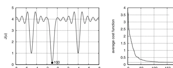
Fig. 1. One-dimensional multimodal function minimisation using the RWBS: (a) cost function, where number 100 beside the point in the graph indicates convergence to the global minimum in all the 100 experiments, and (b) convergence performance averaged over 100 experiments.

ξB = 0.02as well asNG > 6, the RWBS algorithm consistently converged to the global minimum point at u = −1 in all the 100 experiments conducted, as can be seen from the convergence performance shown in Fig. 1 (b). The averaged number of cost function evaluations required for the algorithm to converge to the global optimal solution is around 100, which is consistent with what can be achieved using GA and ASA for this type of one-dimensional optimisation.

Example 2. The IIR filter with transfer functionHM(z)was used to identify the system with transfer functionHS(z)by minimising the mean square error (MSE)J(u), where

HS(z) = 0.05−0.4z

−1

1−1.1314z−1_{+ 0.25z}−2, HM(z) =

a0 1 +b1z−1

(7)

andu = [a0 b1]T. When the system input is white and the noise is absent, the MSE

cost function has a global minimum atuglobal= [−0.311 −0.906]T with the value of

the normalised MSE0.2772and a local minimum atulocal = [0.114 0.519]T with the

normalised MSE value0.9762[11]. In the population initialisation, the parameters were uniformly randomly chosen as(a0, b1)∈(−1.0, 1.0)×(−0.999,0.999). It was found

empirically thatPS = 4,ξB = 0.05NG>15were appropriate, and Fig. 2 (a) depicts convergence performance of the RWBS algorithm averaged over 100 experiments. The previous study [6] applied the ASA to this example. The result of using the ASA is reproduced in Fig. 2 (b) for comparison. The distribution of the solutions obtained in 100 experiments by the RWBS algorithm is shown in Fig. 3.

Example 3. For this 2nd-order IIR filter design, the system and filter transfer functions are given by

HS(z) = −0.3 + 0.4z

−1_−0.5z−2

1−1.2z−1_{+ 0.5z−}2_−0.1z−3, HM(z) =

a0+a1z−1 1 +b1z−1+b2z−2

(8)

0.2 0.3 0.4 0.5 0.6 0.7 0.8 0.9 1

0 50 100 150 200 250 300 350 400 450 500

average cost function

number of function evaluations RWBS global opt

0.2 0.3 0.4 0.5 0.6 0.7 0.8 0.9 1

0 100 200 300 400 500

Averaged Cost Function

Number of Function Evaluations

(a) (b)

Fig. 2. Convergence performance averaged over 100 experiments for the 1st-order IIR filter de-sign: (a) using the RWBS, and (b) using the ASA.

-1 -0.5 0 0.5 1

-1 -0.5 0 0.5 1

y

x

-0.95 -0.94 -0.93 -0.92 -0.91 -0.9 -0.89 -0.88 -0.87

-0.35 -0.34 -0.33 -0.32 -0.31 -0.3 -0.29 -0.28 -0.27

y

x

(a) (b)

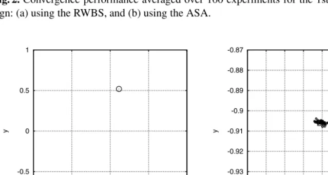
Fig. 3. Distribution of solutions(a0, b1)(small circles) obtained in 100 experiments for the 1st-order IIR filter design by the RWBS: (a) showing the entire search space, and (b) zooming in the global minimum, where large square indicate the global minimum and large circle the local minimum.

The data length used in calculating the MSE cost function was2000. The MSE for this example was multi-modal and the gradient-based algorithm performed poorly as was demonstrated clearly in [6]. In the actual optimisation, the lattice form of the IIR filter was used, and the filter coefficient vector used in optimisation wasu= [a0a1κ0κ1]T,

whereκ0 andκ1 are the lattice-form reflection coefficients. In the population

initial-isation, the parameters were uniformly randomly chosen as ai ∈ (−1.0, 1.0) and κi ∈ (−0.999, 0.999) fori = 0,1. It was found out that NB = 10,ξB = 0.05

0.01 0.1 1

0 100 200 300 400 500 600 700 800 900 1000

average cost function

number of function evaluations RWBS

0.01 0.1 1

0 200 400 600 800 1000

Averaged Cost Function

Number of Function Evaluations

(a) (b)

Fig. 4. Convergence performance for the 2nd-order IIR filter design: (a) using the RWBS averaged over 500 experiments, and (b) using the ASA averaged over 100 experiments.

-1 -0.5 0 0.5 1

-1 -0.5 0 0.5 1

y

x

-2 -1.5 -1 -0.5 0 0.5 1 1.5 2

-2 -1.5 -1 -0.5 0 0.5 1 1.5 2

y

x

(a) (b)

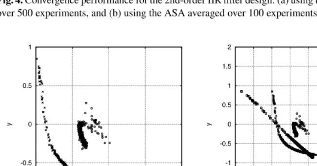
Fig. 5. Distribution of the solutions obtained in 500 experiments for the 2nd-order IIR filter design by the RWBS: (a) showing(a0, a1)as circles and(κ0, κ1)as crosses, and (b) showing(a0, a1)

as circles,(b1, b2)as squares, and(κ0, κ1)as crosses.

of the solutions obtained in 500 experiments by the RWBS is illustrated in Fig. 5. It is clear that for this example there are infinitely many global minima, and the global minimum solutions for(b1, b2)form a one-dimensional space.

Example 4. Consider a blind joint maximum likelihood (ML) channel estimation and data detection for the single-input multiple-output (SIMO) system that employs a single transmitter antenna andL(>1)receiver antennas. In a SIMO system, the symbol-rate sampled antennas’ outputsxl(k),1≤l≤L, are given by

xl(k) = nc−1

i=0

wherenl(k)is the complex-valued Gaussian white noise associated with thelth channel andE[|nl(k)|2_{] = 2σ}2

n,{s(k)}is the transmitted symbol sequence taking values from the quadrature phase shift keying (QPSK) symbol set{±1±j}, andci,lare the channel impulse response (CIR) taps associated with thelth receive antenna. Let

x= [x1(1)x1(2)· · ·x1(N)x2(1)· · ·xL(1)xL(2)· · ·xL(N)]T

s= [s(−nc+ 2)· · ·s(0)s(1)· · ·s(N)]T (10)

c= [c0,1c1,1· · ·cnc−1,1c0,2· · ·c0,Lc1,L· · ·cnc−1,L]

T

be the vector ofN×Lreceived signal samples, the corresponding transmitted data se-quence and the vector of the SIMO CIRs, respectively. The probability density function of the received data vectorxconditioned oncandsis

p(x|c,s) = 1 (2πσ2

n) N L e

− 1

2σ2n

N

k=1

L

l=1|xl(k)−

nc−1

i=0 ci,ls(k−i)|

2

(11)

The joint ML estimate ofcandsis obtained by maximisingp(x|c,s)overcands

jointly. Equivalently, the joint ML estimate is the minimum of the cost function

JML(ˆc,ˆs) = 1

N N

k=1

L

l=1

xl(k)−

nc−1

i=0 ˆ

ci,lsˆ(k−i)

2

(12)

The joint minimisation process(ˆc∗,ˆs∗) = arg [minˆc,ˆsJML(ˆc,ˆs)]can be solved

itera-tively first over the data sequencesˆsand then over all the possible channelscˆ:

(ˆc∗,ˆs∗) = arg

min ˆ c

min

ˆ

s JML(ˆc,ˆs)

(13)

The inner optimisation can readily be carried out using the Viterbi algorithm (VA). We employ the RWBS algorithm to perform the outer optimisation task, and the proposed blind joint ML optimisation scheme can be summarised as follows.

Outer level Optimisation. The RWBS searches the SIMO channel parameter space to find a global optimal estimateˆc∗by minimising the MSEJMSE(ˆc) =JML(ˆc,˜s∗).

Inner level optimisation. Given the channel estimateˆc, the VA provides the ML de-coded data sequence˜s∗, and feeds back the corresponding value of the likelihood metricJML(ˆc,˜s∗)to the upper level.

The SIMO CIRs, listed in Table 1, were simulated with the data lengthN = 50. In practice, the value ofJMSE(ˆc)is all that the upper level optimiser can see, and the

convergence of the algorithm can only be observed through this MSE. In simulation, the performance of the algorithm can also be assessed by the mean tap error defined as

MTE=c−a·ˆc2 (14)

where

a= ±1, ifˆc→ ±c

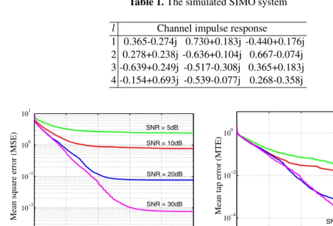
Table 1. The simulated SIMO system

l Channel impulse response 1 0.365-0.274j 0.730+0.183j -0.440+0.176j 2 0.278+0.238j -0.636+0.104j 0.667-0.074j 3 -0.639+0.249j -0.517-0.308j 0.365+0.183j 4 -0.154+0.693j -0.539-0.077j 0.268-0.358j

0 2000 4000 6000 8000 10000 10−3

10−2 10−1 100 101

No. of VA evaluations

Mean square error (MSE)

SNR = 5dB

SNR = 10dB

SNR = 20dB

SNR = 30dB

0 2000 4000 6000 8000 10000 10−4

10−2 100

No. of VA evaluations

Mean tap error (MTE)

SNR = 5dB

SNR = 10dB SNR = 20dB

SNR = 30dB

(a) (b)

Fig. 6. Convergence performance of blind joint ML estimation using the RWBS averaged over 50 runs: (a) MSE and (b) MTE against number of VA evaluations.

0 1000 2000 3000 4000 5000 6000 7000 10−3

10−2 10−1 100 101

No. of VA evaluations

Mean square error (MSE)

SNR = 5dB

SNR = 10dB

SNR = 20dB

SNR = 30dB

0 1000 2000 3000 4000 5000 6000 7000 10−4

10−3 10−2 10−1 100 101

No. of VA evaluations

Mean tap error (MTE)

SNR = 5dB

SNR = 10dB

SNR = 20dB

SNR = 30dB

(a) (b)

Fig. 7. Convergence performance of blind joint ML estimation using the GA averaged over 50 runs: (a) MSE and (b) MTE against number of VA evaluations.

Note that since (ˆc∗,ˆs∗),(−ˆc∗,−ˆs∗),(−jˆc∗,+jˆs∗)and(+jˆc∗,−jˆs∗)are all the solutions of the joint ML estimation problem, the channel estimateˆccan converges to

upper-level optimisation, and the results obtained by this GA-based blind joint ML estimation scheme are presented in Fig. 7. It is worth pointing out that the dimension of the search space wasn= 24for this example.

4

Conclusions

A guided random search optimisation algorithm has been proposed. The local opti-miser in this global search method evolves a population of the potential solutions by forming a convex combination of the solution population with boosting adaptation. A repeating loop involving a combined elitist and random sampling initialisation strategy is adopted to guarantee a fast global convergence. The proposed guided random search method, referred to as the RWBS, is remarkably simple, involving minimum software programming effort and having very few algorithmic parameters that require tuning. The versatility of the proposed method has been demonstrated using several examples, and the results obtained show that the proposed global search algorithm is as efficient as the GA and ASA in terms of global convergence speed, characterised by the total number of cost function evaluations required to attend a global optimal solution.

Acknowledgement

S. Chen wish to thank the support of the United Kingdom Royal Academy of Engineering.

References

1. J.H. Holland, Adaptation in Natural and Artificial Systems. University of Michigan Press: Ann Arbor, MI, 1975.

2. D.E. Goldberg, Genetic Algorithms in Search, Optimization and Machine Learning. Addison Wesley: Reading, MA, 1989.

3. L. Davis, Ed., Handbook of Genetic Algorithms. Van Nostrand Reinhold: New York, 1991. 4. A. Corana, M. Marchesi, C. Martini and S. Ridella, “Minimizing multimodal functions of

continuous variables with the simulated annealing algorithm,” ACM Trans. Mathematical

Software, Vol.13, No.3, pp.262–280, 1987.

5. L. Ingber and B. Rosen, “Genetic algorithms and very fast simulated reannealing: a compar-ison,” Mathematical and Computer Modelling, Vol.16, No.11, pp.87–100, 1992.

6. S. Chen and B.L. Luk, “Adaptive simulated annealing for optimization in signal processing applications,” Signal Processing, Vol.79, No.1, pp.117–128, 1999.

7. R.E. Schapire, “The strength of weak learnability,” Machine Learning, Vol.5, No.2, pp.197– 227, 1990.

8. Y. Freund and R.E. Schapire, “A decision-theoretic generalization of on-line learning and an application to boosting,” J. Computer and System Sciences, Vol.55, No.1, pp.119–139, 1997. 9. R. Meir and G. R¨atsch, “An introduction to boosting and leveraging,” in: S. Mendelson and A. Smola, eds., Advanced Lectures in Machine Learning. Springer Verlag, 2003, pp.119–184. 10. F. Schoen, “Stochastic techniques for global optimization: a survey of recent advances,” J.

Global Optimization, Vol.1, pp.207–228, 1991.