Time variability of sea surface parameters in the tropical Atlantic using satellite and in situ data

(1)

ePrints Soton

Copyright © and Moral Rights for this thesis are retained by the author and/or other

copyright owners. A copy can be downloaded for personal non-commercial

research or study, without prior permission or charge. This thesis cannot be

reproduced or quoted extensively from without first obtaining permission in writing

from the copyright holder/s. The content must not be changed in any way or sold

commercially in any format or medium without the formal permission of the

copyright holders.

When referring to this work, full bibliographic details including the author, title,

awarding institution and date of the thesis must be given e.g.

AUTHOR (year of submission) "Full thesis title", University of Southampton, name

of the University School or Department, PhD Thesis, pagination

(2)

FACULTY OF ENGINEERING, SCIENCE & MATHEMATICS

Southampton Oceanography Centre

School of Ocean & Earth Sciences

Time variability of sea surface parameters in the

tropical Atlantic using satellite and in situ data

by

Antonio Caetano Vaz Caltabiano

Thesis for the degree of Doctor of Philosophy

September 2004

(3)

This PhD dissertation by

Antonio Caetano Vaz Caltabiano

has been produced under the supervision of the following persons

Supervisor

Professor Ian S. Robinson

Chair of Advisory Panel

Professor Michael Collins

Member of Advisory Panel

(4)

ABSTRACT

FACULTY OF ENGINEERING, SCIENCE & MATHEMATICS

SCHOOL OF OCEAN & EARTH SCIENCES

Doctor of Philosophy

TIME VARIABILITY OF SEA SURFACE PARAMETERS IN THE TROPICAL

ATLANTIC USING SATELLITE AND IN SITU DATA

by Antonio Caetano Vaz Caltabiano

The influence of the tropical Atlantic Ocean over the climate of Europe, Africa and America is well known today. However, several questions about high-frequency processes in this region remain open. This thesis addresses the characterisation of the diurnal and other short timescale variability of the meteo-ocean variables measured in the tropical Atlantic Ocean by the PIRATA array, as well as derived air-sea heat fluxes. By combining the complementarity and mitigating the disadvantages of using the high temporal resolution of in situ data in conjunction with the excellent spatial coverage of satellite based data, this work also aims to investigate the characteristics of the Tropical Instability Waves in the tropical Atlantic. The satellite data validation process used in this study assesses each of the buoys individually, to take into account possible regional biases.

A complete picture of the mean diurnal cycle and the seasonal variability of the diurnal signal is performed for the first time for the whole tropical Atlantic basin. The SST diurnal signal presents strong characteristics during the respective summer in both hemispheres. However, through the wavelet technique used in this analysis, a significant diurnal signal at the equator could be noticed during the second half of each year, indicating a possible modulation of the diurnal signal by processes with different timescales. It is suggested that Tropical Instability Waves could be one of these processes. The results presented here show that the TIW clearly vary their position and time of activity, depending on the degree of development of the equatorial cold tongue. The most active year analysed in this study was 2001, when the spectral characteristics could be observed as far north as 4oN. The imprints of the TIW are well marked in the wind fields, showing that clearly there are coupled mechanisms associated with the TIW. Moreover, this study confirms that a coupling mechanism suggested for the Pacific Ocean is also applicable to the tropical Atlantic basin. The measurements made by the TMI sensor, in conjunction with the Qscat wind data showed that the atmospheric fields are highly correlated with the SST fields at the timescale associated with the TIW.

(5)

LIST OF FIGURES ... iv

LIST OF TABLES ... xiii

DECLARATION OF AUTHORSHIP ... xiv

ACKNOWLEDGEMENTS ... xv

ACRONYMS ... xvi

CHAPTER 1 - INTRODUCTION

1.1 – General Introduction ... 1 - 1 1.2 – Objectives ... 1 - 6 1.3 – Structure of the document ... 1 - 8

CHAPTER 2 – VARIABILITY OF THE TROPICAL ATLANTIC

2.1 – Introduction ... 2 - 1 2.2 – Winds... 2 - 1 2.3 – Sea surface temperature... 2 - 4 2.4 – Currents ... 2 - 7 2.5 – Air-sea fluxes ... 2 - 12 2.6 – Current knowledge of TIW ... 2 - 14 2.6.1 – TIW in the tropical Atlantic... 2 - 17 2.7 – Summary ... 2 - 18

CHAPTER 3 – DATASET AND METHODS OF ANALYSIS

(6)

3.4 – Analytical Methods ... 3 - 15 3.4.1 – Radon Transform (RT) ... 3 - 16 3.4.2 – Wavelets ... 3 - 17 3.5 – Summary ... 3 - 20

CHAPTER 4 – VALIDATION OF THE DATASET

4.1 – Introduction ... 4 - 1 4.2 – Impact of availability of data ... 4 - 2 4.3 – Wind data... 4 - 2 4.4 – Sea surface temperature... 4 - 23 4.5 – Heat fluxes ... 4 - 34 4.6 – Summary ... 4 - 36

CHAPTER 5 – DIURNAL CYCLE IN THE TROPICAL OCEANS

5.1 – Introduction ... 5 - 1 5.2 – Current knowledge of the diurnal cycle ... 5 - 2 5.2.1 – Winds ... 5 - 2 5.2.2 – Sea Surface Temperature ... 5 - 3 4.2.3 – Air-sea fluxes ... 5 - 5 5.3 – Diurnal variability in the tropical Atlantic ... 5 - 7 5.3.1 – Mean diurnal cycle ... 5 - 7 5.3.2 - Seasonal variation of the diurnal cycle ... 5 - 15 5.4 – Impact of daily wind on hourly surface heat fluxes ... 5 - 29 5.5 – Diurnal variability of heat fluxes in the Tropical Atlantic ... 5 - 36 5.5.1 – Mean diurnal cycle ... 5 - 36 5.5.2 – Seasonal variation of the diurnal cycle of heat fluxes ... 5 - 39 5.6 – Summary ... 5 - 45

CHAPTER 6 – TROPICAL INSTABILITY WAVES

(7)

CHAPTER 7 – INTERACTIONS BETWEEN DIURNAL VARIABILTY AND TIW

7.1 – Introduction ... 7 - 1 7.2 – Diurnal amplitude and TIW relationship... 7 - 3 7.3 – Summary ... 7 - 13

CHAPTER 8 – DISCUSSION, CONCLUSIONS AND FUTURE WORK

8.1 – General Discussion ... 8 - 1 8.2 – Conclusions ... 8 - 5 8.3 – Future work ... 8 - 6

(8)

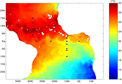
Figure 1.1 - Position of the buoys in the PIRATA array (black points) Overlaying TMI SST (colour) on a 3-day mean composite starting on

19/09/2001. SST is in oC... 1 - 3 Figure 2.1 - Wind stress annual mean. Source: SOC Climatology

(http://www.soc.soton.ac.uk/JRD/MET/fluxclimmon.php) ... 2 - 2 Figure 2.2 – SST annual cycle with amplitude (contours and length of

vectors) and phase (direction of vectors). An arrow that is pointing straight up indicates maximum occurs in January. Phase increases clockwise.

Contour interval is 1o C. Source: Carton and Zhou (1997).. ... 2 - 5 Figure 2.3 – Schematic diagram of the tropical surface water layer (TSW)

in the Atlantic Ocean during boreal spring (upper panel) and boreal

autumn (lower panel). Adapted from Stramma and Schott (1999)... 2 - 10

Figure 2.4 – Schematic diagram of the mean Central Water layer (CW) in

the Atlantic Ocean. Adapted from Stramma and Schott (1999). ... 2 - 11 Figure 2.5 – Schematic representation of perturbation of the surface wind

field (U = zonal wind, V = meridional wind) associated with a TIW, following the hypothesis suggested by Lindzen and Nigam (1987) (top panel) and Wallace et al. (1989) (bottom panel). Arrows in the figure

represent wind. Figure modified from Hayes et al. (1989) ... 2 - 16 Figure 3.1 – The Next Generation ATLAS mooring (Source: TAO Project

Website) ... 3 - 3 Figure 3.2 – Position of the buoys in the PIRATA array... 3 - 4 Figure 3.3 – Availability of the PIRATA dataset ... 3 - 5 Figure 3.4 – Schematic of the 2D RT of a longitude-time section modified

from Challenor et al. ( 2001) ... 3 - 17 Figure 4.1 – Comparison between buoy wind speed and satellite wind

speed. Satellite wind data is TMI 11GHz (red), TMI 37GHz (blue) and

Qscat (black). ... 4 - 3 Figure 4.2 – Wind speed (ms-1) measured by PIRATA buoys (X axis) and

QuikSCAT (Y axis)... 4 - 5 Figure 4.3 – Wind speed (ms-1) measured by PIRATA buoys (X axis) and

TMI 11 GHz (Y axis) ... 4 - 5 Figure 4.4 - Wind speed (ms-1) measured by PIRATA buoys (X axis) and

TMI 37 GHz (Y axis) ... 4 - 6 Figure 4.5 – Dependence of wind speed residual (Buoy – satellite) on the

buoy wind speed. Satellite wind data is TMI 11GHz (red), TMI 37GHz

(9)

TMI 37GHz (bottom) ... 4 - 9 Figure 4.7 – Dependence of wind speed residual (Buoy – QuikSCAT) on

the buoy wind speed. (Upper panels) Scatterplots and (lower panels) number of data points, averages (points) and standard error (vertical

lines) calculated in bins of buoy wind speed of 1 ms-1. ... 4 - 10 Figure 4.8 – Dependence of wind speed residual (Buoy – TMI 11 GHz)

on the buoy wind speed. (Upper panels) Scatterplots and (lower panels) number of data points, averages (points) and standard error (vertical

lines) calculated in bins of buoy wind speed of 1 ms-1. ... 4 - 11

Figure 4.9 – Dependence of wind speed residual (Buoy – TMI 37 GHz) on the buoy wind speed. (Upper panels) Scatterplots and (lower panels) number of data points, averages (points) and standard error (vertical

lines) calculated in bins of buoy wind speed of 1 ms-1. ... 4 - 12 Figure 4.10 – Dependence of wind speed residual (Buoy – satellite) on

the buoy SST. Satellite wind data is TMI 11GHz (red), TMI 37GHz (blue)

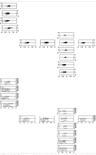
and Qscat (black)... 4 - 13 Figure 4.11 – Dependence of wind speed residual (buoy – satellite) on

buoy SST. Number of data points (histograms), averages (points) and standard error (vertical lines) calculated in bins of SST of 0.5oC for wind data retrieved from Qscat (top), TMI 11GHz (middle) and TMI 37GHz

(bottom) ... 4 - 14 Figure 4.12 – Dependence of wind speed residual (Buoy – satellite) on

the buoy air-sea temperature difference. Satellite wind data is TMI 11GHz

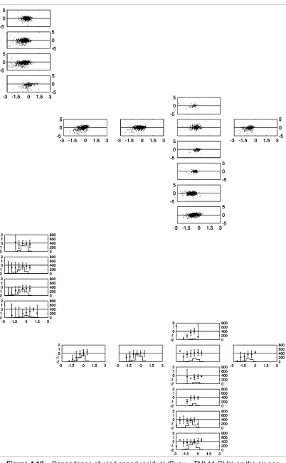
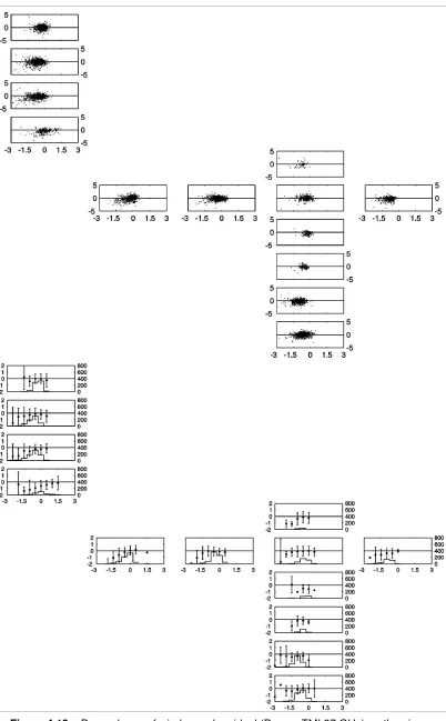
(red), TMI 37GHz (blue) and Qscat (black). ... 4 - 14 Figure 4.13 – Dependence of wind speed residual (buoy – satellite) on

buoy air-sea temperature difference. Number of data points (histograms), averages (points) and standard error (vertical lines) calculated in bins of air-sea temperature difference of 0.5oC for wind data retrieved from Qscat

(top), TMI 11GHz (middle) and TMI 37GHz (bottom) ... 4 - 15 Figure 4.14 – Dependence of wind speed residual (Buoy – QuikSCAT)

on the SST. (Upper panels) Scatterplots and (lower panels) number of data points, averages (points) and standard error (vertical lines)

calculated in bins of SST of 0.5 oC ... 4 - 17 Figure 4.15 – Dependence of wind speed residual (Buoy – TMI 11 GHz)

calculated in bins of SST of 0.5 oC ... 4 - 18 Figure 4.16 – Dependence of wind speed residual (Buoy – TMI 37 GHz)

(10)

(lower panels) number of data points, averages (points) and standard error (vertical lines) calculated in bins of air-sea temperature difference of

0.5 oC... 4 - 20 Figure 4.18 – Dependence of wind speed residual (Buoy – TMI 11 GHz)

on the air-sea temperature difference. (Upper panels) Scatterplots and (lower panels) number of data points, averages (points) and standard error (vertical lines) calculated in bins of air-sea temperature difference of

0.5 oC... 4 - 21

Figure 4.19 – Dependence of wind speed residual (Buoy – TMI 37 GHz) on the air-sea temperature difference. (Upper panels) Scatterplots and (lower panels) number of data points, averages (points) and standard error (vertical lines) calculated in bins of air-sea temperature difference of

0.5 oC... 4 - 22 Figure 4.20 – (a) Comparison between buoy-measured SST at 1 metre

and skin-derived SST. (b) Dependence of T (skin – buoy) on buoy wind speed with number of data in units of 104 (histogram), averages (points) and standard error (vertical lines) calculated in bins of buoy wind speed of 1 ms-1 for all data. (c) As (b) but only for daytime data. (d) As (b) but only

for nighttime data (d)... 4 - 25 Figure 4.21 – Comparison between buoy-measured SST (X axis) at

1 metre and skin-derived SST (Y axis) for each individual buoy... 4 - 26 Figure 4.22 - T (skin SST – SST) as function of buoy wind speed.

Number of data points (right-Y axis) in 103 units, averages (points) and standard error (vertical lines) calculated in bins of buoy wind speed of

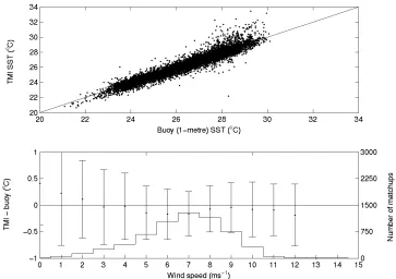
1 ms-1... 4 - 28 Figure 4.23 – Comparison between buoy-measured SST at 1 metre and

TMI SST (upper panel). Dependence of T (TMI – buoy) on buoy wind speed with number of data (histogram), averages (points) and standard error (vertical lines) calculated in bins of buoy wind speed of 1 ms-1 (lower

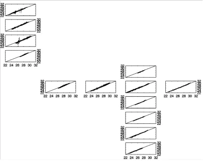
panel). ... 4 - 29 Figure 4.24 – Comparison between buoy-measured SST (X axis) at

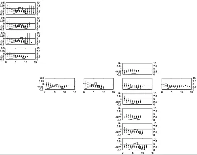
1 metre and TMI-retrieved SST (Y axis) for each individual buoy... 4 - 30 Figure 4.25 - T (TMI – buoy) as function of buoy wind speed. Number of

data points (right-Y axis), averages (points) and standard error (vertical

lines) calculated in bins of buoy wind speed of 1 ms-1. ... 4 - 31 Figure 4.26 – Comparison between skin-derived SST and TMI SST

(upper panel). Dependence of T (TMI – skin) on buoy wind speed with number of data (histogram), averages (points) and standard error (vertical

lines) calculated in bins of buoy wind speed of 1 ms-1 (lower panel)... 4 - 32 Figure 4.27 – Comparison between skin-derived SST (X axis) and

(11)

Figure 5.1 – TB (solid line) andTS (dotted line) mean diurnal cycle in the

tropical Atlantic. Y-axis shows values in oC. X-axis is given in hours... 5 - 8 Figure 5.2 – Wind speed mean diurnal cycle in the tropical Atlantic.

Y-axis shows values in ms-1. X-axis is given in hours... 5 - 10 Figure 5.3 – Zonal wind mean diurnal cycle in the tropical Atlantic.

Y-axis shows values in ms-1. X-axis is given in hours... 5 - 11 Figure 5.4 – Meridional wind mean diurnal cycle in the tropical Atlantic.

Y-axis shows values in ms-1. X-axis is given in hours... 5 - 12 Figure 5.5 – Mean diurnal cycle of SST (solid), skin SST (dotted) and

wind speed (dashed). Units are oC for SST and skin SST, and ms-1 for

wind speed. ... 5 - 12 Figure 5.6 – Mean diurnal cycle of SST (solid), skin SST (dotted) and

wind speed change ((wind)/t) (dashed). Units are oC for SST and

skin-SST, and ms-1 hr-1 for wind speed change. ... 5 - 13 Figure 5.7 – Air temperature mean diurnal cycle in the tropical Atlantic.

Y-axis shows values in oC. X-axis is given in hours... 5 - 13 Figure 5.8 – Air-sea temperature difference mean diurnal cycle in the

tropical Atlantic. Y-axis shows values in oC. X-axis is given in hours... 5 - 14 Figure 5.9 – Relative humidity mean diurnal cycle in the tropical Atlantic.

Y-axis shows values in %. X-axis is given in hours. ... 5 - 15 Figure 5.10 – Detail of SST wavelet power spectra for the buoy at

0oN 23oW (top panel). 16 – 32 hours band average time series (lower panel). Black contour lines in the upper panel and dashed line in the

lower panel are the 95% confidence level. Units are (oC)2... 5 - 16 Figure 5.11a – SST wavelet power spectra for the PIRATA buoys. Y-axis

is the period in hours. The colorbar unit is (oC) 2, as in Figure 5.11c. Black

contour lines are the 95% confidence level. ... 5 - 18 Figure 5.11b – SST wavelet power spectra for the PIRATA buoys. Y-axis

is the period in hours. The colorbar unit is (oC) 2. Black contour lines are

the 95% confidence level. ... 5 - 19

Figure 5.11c – SST wavelet power spectra for the PIRATA buoys. Y-axis is the period in hours. The colorbar unit is (oC) 2. Black contour lines are

the 95% confidence level. ... 5 - 20

Figure 5.12a – Wind speed wavelet power spectra for the PIRATA buoys. Y-axis is the period in hours. The colorbar unit is (m/s) 2. Black contour

(12)

contour lines are the 95% confidence level. ... 5 - 22 Figure 5.12c – Wind speed wavelet power spectra for the PIRATA buoys.

Y-axis is the period in hours. The colorbar unit is (m/s) 2. Black contour

lines are the 95% confidence level. ... 5 - 23 Figure 5.13a – Air temperature wavelet power spectra for the PIRATA

buoys. Y-axis is the period in hours. The colorbar unit is (oC) 2. Black

contour lines are the 95% confidence level. ... 5 - 24

Figure 5.13b – Air temperature wavelet power spectra for the PIRATA buoys. Y-axis is the period in hours. The colorbar unit is (oC) 2. Black

contour lines are the 95% confidence level. ... 5 - 25

Figure 5.13c – Air temperature wavelet power spectra for the PIRATA buoys. Y-axis is the period in hours. The colorbar unit is (oC) 2. Black

contour lines are the 95% confidence level.. ... 5 - 26 Figure 5.14a – Relative humidity wavelet power spectra for the PIRATA

buoys. Y-axis is the period in hours. The colorbar unit is (%) 2. Black

contour lines are the 95% confidence level. ... 5 - 27 Figure 5.14b – Relative humidity wavelet power spectra for the PIRATA

contour lines are the 95% confidence level. ... 5 - 28 Figure 5.14c – Relative humidity wavelet power spectra for the PIRATA

contour lines are the 95% confidence level. ... 5 - 29 Figure 5.15 – Hourly latent heat flux (Wm-2) calculated using hourly wind

speed (X axis) and daily wind speed (Y axis) ... 5 - 31 Figure 5.16 – Hourly sensible heat flux (Wm-2) calculated using

hourly wind speed (X axis) and daily wind speed (Y axis). ... 5 - 31 Figure 5.17 – Dependence of latent heat flux residuals on the buoy wind

speed. Number of data points, averages (points) and standard error

(vertical lines) calculated in bins of wind speed of 1 ms-1. ... 5 - 32 Figure 5.18 – Dependence of latent heat flux residuals on SST. Averages

(points) calculated in bins of SST of 0.5 oC. ... 5 - 33 Figure 5.19 – Mean diurnal cycle of sensible heat flux calculated using

hourly (solid line) and daily (circles) wind speed. X-axis is time (hours)

and Y-axis is Qsen (Wm-2) ... 5 - 34

Figure 5.20 – Mean diurnal cycle of latent heat flux calculated using hourly (solid line) and daily (circles) wind speed. X-axis is time (hours)

and Y-axis is Qsen (Wm-2).. ... 5 - 35

Figure 5.21 – Mean diurnal cycles of latent flux differences using hourly

(13)

Figure 5.23 – Mean diurnal cycle of latent heat flux in the tropical Atlantic.

X-axis is given in hours. Y-axis shows values in Wm-2. ... 5 - 38 Figure 5.24a – Sensible heat flux wavelet power spectra for the PIRATA

buoys. Y-axis is the period in hours. The colorbar unit is (Wm-2)2. Black

contour lines are the 95% confidence level. ... 5 - 40 Figure 5.24b – Sensible heat flux wavelet power spectra for the PIRATA

contour lines are the 95% confidence level. ... 5 - 41 Figure 5.24c – Sensible heat flux wavelet power spectra for the PIRATA

contour lines are the 95% confidence level.. ... 5 - 42 Figure 5.25a – Latent heat flux wavelet power spectra for the PIRATA

contour lines are the 95% confidence level ... 5 - 43 Figure 5.25b – Latent heat flux wavelet power spectra for the PIRATA

contour lines are the 95% confidence level.. ... 5 - 44 Figure 5.25c – Latent heat flux wavelet power spectra for the PIRATA

contour lines are the 95% confidence level. ... 5 - 45 Figure 6.1 – Example of TMI SST 3-day mean composites for the years

of 1998, 1999, 2000 and 2001.. ... 6 - 2 Figure 6.2 – Time-longitude plots of TMI SST data at the Equator, 1oN,

2oN, 3o N and 4oN. SST is in oC. Black lines show the position and length

of the SST data from the PIRATA buoys... 6 - 3 Figure 6.3 – Time-longitude plots of filtered TMI SST data at the Equator,

1oN, 2oN, 3o N and 4oN. SST is in oC. Black lines show the position and

length of the SST data from the PIRATA buoys.. ... 6 - 5 Figure 6.4 – Standard deviation of SST for several latitudes at the

tropical Atlantic Ocean. Top left panel shows the standard deviation of the time series spanning from 1998 to 2001 for the latitudes of equator, 1oN, 2oN, 3oN and 4oN.The remaining panels are each zonally averaged for the

same latitudes as above, and for the different years. ... 6 - 6 Figure 6.5 – Time-longitude plots of Qscat wind speed data at the

equator, 1oN, 2oN, 3o N and 4oN. Wind speed is in ms-1. Black lines show

(14)

in C (bottom panels). Vertical black lines show the position and length of

the SST data from the PIRATA buoys... 6 - 10 Figure 6.7 – Standard deviation of QuikSCAT wind speed data for

several latitudes at the tropical Atlantic Ocean. Top left panel shows the standard deviation of the time series spanning from 1998 to 2001 for the latitudes of equator, 1oN, 2oN, 3oN and 4oN.The remaining panels are each zonally averaged for the same latitudes as above, and for the

different years. ... 6 - 11

Figure 6.8 – Time-longitude plots of filtered data at the Equator, 1oN, 2oN, 3o N and 4oN for QuikScat zonal wind in ms-1 (top panels) and TMI SST in oC (bottom panels). Vertical black lines show the position and length of

the SST data from the PIRATA buoys... 6 - 12 Figure 6.9 – Time-longitude plots of filtered data at the Equator, 1oN, 2oN,

3o N and 4oN for QuikScat meridional wind in ms-1 (top panels) and TMI SST in oC (bottom panels). Vertical black lines show the position and

length of the SST data from the PIRATA buoys. ... 6 - 14 Figure 6.10 – Standard deviation of QuikSCAT zonal wind for several

latitudes at the tropical Atlantic Ocean. Top left panel shows the standard deviation of the time series spanning from 1998 to 2001 for the latitudes of equator, 1oN, 2oN, 3oN and 4oN.The remaining panels are each zonally

averaged for the same latitudes as above, and for the different years. ... 6 - 15 Figure 6.11 – Standard deviation of QuikSCAT meridional wind for

several latitudes at the tropical Atlantic Ocean. Top left panel shows the standard deviation of the time series spanning from 1998 to 2001 for the latitudes of equator, 1oN, 2oN, 3oN and 4oN.The remaining panels are each zonally averaged for the same latitudes as above, and for the

different years. ... 6 - 15 Figure 6.12 – Regression maps for SST, VAP (mm oC-1),

CLD (10-2 mm oC-1) and rain (mm hr-1 oC-1). SST contours are plotted in all graphs. Vectors are for wind velocity. Black arrow shows wind velocity

approximate to 0.3 m s-1oC-1... 6 - 16 Figure 6.13 – Longitudinal variations at 1oN of the filtered anomalies of

SST (oC), cloud liquid water (CLD) (10-2 mm), integrated water vapour

(VAP) (mm), zonal (U) (ms-1) and meridional (V) (ms-1) wind. ... 6 - 17 Figure 6.14 – Regression maps for SST (colour and contours). Vectors

are for wind velocity. Black arrow shows wind velocity approximate to

0.3 m s-1oC-1. ... 6 - 18 Figure 6.15 – Regression maps for VAP (mm oC-1). Vectors are for wind

velocity. Black arrow shows wind velocity approximate to 0.3 m s-1oC-1.

SST contours from Figure 6.14 are present in all graphs. ... 6 - 19 Figure 6.16 – Regression maps for CLD (10-2 mm oC-1). Vectors are for

wind velocity. Black arrow shows wind velocity approximate to 0.3 m s-1

(15)

Figure 7.1 - Detail of SST wavelet power spectra for the buoy at 0oN 23oW (top panel). 16 – 32 hours band average time series (lower panel). Black contour lines in the upper panel and dashed line in the lower panel

are the 95% confidence level. Units are (oC)2... 7 - 2 Figure 7.2 – Relationship between diurnal signal and 20-40 day period at

0oN 0oW. (a) Band-average variance of SST within the diurnal band (solid line) and 20-40 day band (dashed line). (b) Time series of the 20-40 day components for diurnal amplitude of SST (solid line) and diurnal

amplitude of skin-SST (dashed line). (c) Same as (b) but for wind speed. (d) Same as (b) but for diurnal amplitude of sensible heat flux (solid line) and latent heat flux (dashed line). Horizontal lines in (b), (c) and (d) are

the 95% confidence limits. ... 7 - 6 Figure 7.3 – Relationship between diurnal signal and 20-40 day period at

0oN 10oW. (a) Band-average variance of SST within the diurnal band (solid line) and 20-40 day band (dashed line). (b) Time series of the 20-40 day components for diurnal amplitude of SST (solid line) and diurnal amplitude of skin-SST (dashed line). (c) Same as (b) but for wind speed. (d) Same as (b) but for diurnal amplitude of sensible heat flux (solid line) and latent heat flux (dashed line). Horizontal lines in (b), (c) and (d) are

the 95% confidence limits. ... 7 - 9 Figure 7.6 – Cross correlation between SST diurnal amplitude and wind

speed (solid line) and skin-SST diurnal amplitude and wind speed (dashed line) on a 20-40 day timescale for the PIRATA buoys on the equator. Positive time lag means SST leads wind. Horizontal dotted lines

(16)

skin-SST and diurnal amplitude of latent heat flux (dashed line) on a 20-40 day timescale for the PIRATA buoys on the equator. Positive time lag means SST leads latent heat. Horizontal dotted lines are the 95%

(17)

Table 3.1 – Details of sensors at the Next Generation ATLAS moorings.

Source: TAO Project website ... 3 - 4 Table 4.1 – Statistics of comparison between wind speed (ms-1)

measured by PIRATA buoys and QSCAT... 4 - 6 Table 4.2 – Statistics of comparison between wind speed (ms-1)

measured by PIRATA buoys and TMI 11 GHz ... 4 - 7 Table 4.3 – Statistics of comparison between wind speed (ms-1)

measured by PIRATA buoys and TMI 37 GHz ... 4 - 7 Table 4.4 – Statistics of comparison between SST and skin-SST (oC)... 4 - 26 Table 4.5 – Statistics of comparison between SST and TMI (oC) ... 4 - 30

Table 4.6 – Statistics of comparison between TMI-retrieved and

skin-SST (oC) ... 4 - 33 Table 4.7 – Rms difference of Qlat and Qlon associated with errors in the

measurement of bulk variables. ... 4 - 36 Table 5.1 – TB and TS diurnal amplitude and their ratio ... 5 - 9 Table 5.2 – Statistics of comparison between Qlat and Qsen calculated with

(18)

I, Antonio Caetano Vaz Caltabiano,

declare that the thesis entitled

Time variability of sea surface parameters in the tropical Atlantic using satellite

and in situ data

and the work presented in it are my own. I confirm that:

this work was done wholly or mainly while in candidature for a research

degree at this University;

where any part of this thesis has previously been submitted for a degree or

any other qualification at this University or any other institution, this has

been clearly stated;

where I have consulted the published work of others, this is always clearly

attributed;

where I have quoted from the work of others, the source is always given.

With the exception of such quotations, this thesis is entirely my own work;

I have acknowledged all main sources of help;

where the thesis is based on work done by myself jointly with others, I have

made clear exactly what was done by others and what I have contributed

myself;

none of this work has been published before submission.

Signed: ………..

(19)

I would not be able to finish this thesis without the help and support of several people. For this I would like to thanks:

• My supervisor, Professor Ian Robinson, and the members of my panel, Professor Michael Collins and Dr Neil Wells;

• Ministério da Ciência e Tecnologia – Brasil, through Conselho Nacional de Desenvolvimentto Científico e Tecnológico (CNPq) for financial support during my candidature;

• The whole LSO group for allowing me to use its facilities and for storing all satellite data used in this thesis. Remote Sensing Systems (http://www.ssmi.com/) for providing TMI and QuikScat datasets. TAO Project Office for providing the PIRATA (http://www.pmel.noaa.gov/pirata/) dataset. Wavelet software was provided by C. Torrence and G. Compo (http://paos.colorado.edu/research/wavelets/);

• A very special thanks to David Cromwell for all his support and friendship during all my time here, in particular at the end by revising the whole document. Also, many thanks to Christine, Cipo, Helen, Lisa, Graham, Peter, Richenda and Andrew for their friendship and help with Matlab, data management, maths, data processing, etc… • Alice Stuart-Menteth for her friendship and for always being there for discussing things. And for listening.

• My friends in Southampton (and some who moved on): Susanne and Hans, Boris and Tamaris (+ Rozanna and Natalia), Martin, Ollie, James, Isabel and Carlos, Dohyung, Ana Hilário, Xana, Maria, Dave Lambkin, Babete and Alex, Sinhue and Sara, Adriana and Ben, Anita and Alessio, Taro and Alessandra;

• The “Brazilian Gang”: Ronald and Tati (+ Bela and Flora), Rodrigo and Dhesi (+ Henrique and Isadora), Alex and Valéria (+ Gabriel and Vinícius), Lu and Marisa, César and Sílvia (+ Vìtor), Hervé and Ana (+Pierre), Olliand Sílvia, Erik and Roberta, Gilberto and Elisa (+ Júlia), Marcos and Caína, James, Edu and Cláudia, and Manu; • Família Veeck, pelo carinho e amizade que me receberam dentro de casa. Não fazem idéia de como foram importantes!!

• Meus pais, pela vida e por estarem presentes sempre que precisei. E minhas irmãs, pela amizade e felicidade de ser um irmão;

(20)

ACCE Atlantic Circulation and Climate Experiment ADEOS Advanced Earth Observing Satellite

ATLAS Autonomous Temperature Line Acquisition System ATSR Along-Track Scanning Radiometer

AVHRR Advanced Very High Resolution Radiometer

BC Brazil Current

CCM3 NCAR Community Climate Model COADS Comprehensive Ocean-Atmosphere Data Set

COARE Coupled Ocean Atmosphere Response Experiment cSEC central South Equatorial Current

CW Central Waters

DAS Data Assimilation System

DWBC Deep Western Boundary Current

ECMWF European Centre for Medium-Range Weather Forecasts ENSO El Niño Southern Oscillation

EOF Empirical Orthogonal Functions

eSEC equatorial South Equatorial Current

EUC Equatorial Undercurrent

FOCAL Français Océan Climat Atlantique Equatorial GARP Global Atmospheric Research Program GATE GARP Atlantic Tropical Experiment

GC Guinea Current

GEOS Goddard Earth Observing System

GHRSST-PP GODAE High Resolution Sea Surface Temperature Pilot Project GODAE Global Ocean Data Assimilation Experiment

ITCZ Intertropical Convergence Zone NAO North Atlantic Oscillation

NASA National Aeronautics and Space Administration

NBC North Brazil Current

NCAR National Center for Atmospheric Research NCEP National Centers for Environmental Prediction NEC North Equatorial Current

NECC North Equatorial Countercurrent

NSCAT NASA Scatterometer

(21)

RT Radon Transform

SEC South Equatorial Current

SECC South Equatorial Countercurrent SEQUAL Seasonal Response of the Equatorial Atlantic SEUC South Equatorial Undercurrent SMMI Special Sensor Microwave/Imager

SMMR Scanning Multichannel Microwave Radiometer sSEC southern South Equatorial Current

SST Sea Surface Temperature

SVD Singular Value Decomposition

TAO Tropical Atmosphere/Ocean

TIW Tropical Instability Waves

TMI TRMM Microwave Imager

TOGA Tropical Ocean Global Atmosphere

TRMM Tropical Rainfall Measuring Experiment

TSW Tropical Surface Water

VOS Volunteer Observing Ship

(22)

C h a p te r 1

Introduction

1.1. General introduction

The tropical oceans are generally characterised by a relatively shallow thermocline (about 100 m deep) separating a layer of warm, light fluid from a cooler, heavier one. The tropical ocean’s upper layer can be defined by two parameters: surface temperature and thermocline depth. The depth of the thermocline is considered as the dynamic response of the ocean to the global wind forcing, and the surface temperature is mostly considered as the thermodynamic response of the ocean to the local thermodynamic atmospheric forcing. Maintained by permanent easterly tradewinds, the annual mean thermocline is deeper on the western than on the eastern side of the tropical ocean (Merle and Arnault, 1985; Carton and Zhou, 1997).

(23)

tropical Atlantic, particular emphasis has been given to the study of the sea surface temperature (SST) oscillation known as the tropical Atlantic dipole (Servain, 1991) and its relation to the regional and world climate.

The lack of in situ data in the Tropical Atlantic has always been one of the major obstacles to a better understanding of the variability in the region. The first two major projects set up to consistently collect and analyse oceanographic and meteorological data in this region were the Global Atmospheric Research Program (GARP) Atlantic Tropical Experiment (GATE) in 1974, and the Français Océan Climat Atlantique Equatorial / Seasonal Response of the Equatorial Atlantic (FOCAL/SEQUAL) project, established in 1982. In the late 1990’s, the establishment of research projects such as the Atlantic Circulation and Climate Experiment (ACCE) (WOCE, 1997) and the Pilot Research Moored Array in the Tropical Atlantic (PIRATA) (Servain et al., 1998) has increased the number and quality of data in the tropical Atlantic.

The PIRATA program began in late 1997 with the full array in place by the year 2000. It was envisioned as part of a multinational effort involving Brazil, France, and the United States. The array consists of 13 Next Generation ATLAS (Autonomous Temperature Line Acquisition System) moorings spanning 15oN – 10oS, 38oW – 0o (Figure 1.1). Of these 13 buoys initially proposed to be deployed, only 11 are still acquiring and transmitting the data. The loss of the other 2 buoys (2oN and 2oS at 10oW) is due to vandalism associated with tuna fishing, which takes place in the eastern equatorial Atlantic. The specific configuration of the PIRATA array (Figure 1.1) has been chosen to provide coverage along the equator of regions of strong wind forcing in the western basin and significant seasonal-to-interannual variability in SST in the central and eastern basin. The spacing of moorings near the equator (10o – 15o zonally and 2o meridionally) has been chosen to resolve the rapid equatorial Kelvin wave responses to abrupt wind changes in the western Atlantic.

(24)

[image:24.595.110.537.123.419.2]

temporal and spatial resolutions required to study the tropical rapid and large-scale variations.

Figure 1.1 – Position of the buoys in the PIRATA array (black points) overlaying TMI SST (colour) on a 3-day mean composite starting on 19/09/2001. SST is in oC.

Satellite sensors provide an alternative approach to measuring SST from ships, and provide the higher spatial and temporal coverage needed to generate climatology more capable of characterizing local and seasonal SST changes, over time scales of days to years and spatial scales of a few kilometres. If used in conjunction with in situ data, i.e. from ships, moored buoys and drifters, the measurements from satellite sensors become a very powerful tool to understand many oceanographic phenomena.

(25)

opportunity generally obtain SST from a layer of about 5 – 10 metres deep. This is an important point because the temperature of the surface skin can differ by up to several degrees from the bulk SST (Yokoyama et al., 1995; Soloviev and Lukas, 1997; Donlon et al., 1999), being typically slightly cooler than the water millimetres below it by 0.17oC (Donlon et al., 2002). As these previous studies have clearly shown that the diurnal signal has the potential to add bias and noise to measurements supposed to represent the mixed layer SST, Donlon (2004), through the GODAE High Resolution Sea Surface Temperature Pilot Project (GHRSST-PP), suggested a new definition for SST to describe the true mixed layer surface temperature, called Foundation Temperature. The project also recommends that all in situ measurements should be defined with their depth. For the present work, the term of bulk SST always refers to buoy measurements at 1-m depth.

The difference between bulk and skin SST is mainly due to the combined effects of diurnal warming and the “skin effect” (which is due to the effects of radiative and evaporative heat loss). The radiative, latent, and sensible heat exchanges between the atmospheric and oceanic boundary layers depend on the actual skin temperature of the ocean, making the skin temperature the critical SST for examining air-sea interactions (Webster et al., 1996).

Most of the databases that contain satellite infra-red SST data have their calibration algorithms built in reference to in situ SST measured by buoys or ships of opportunity. Once this is done, important processes such as the skin effect are incorporated to the data set (Robinson et al., 1984). Casey and Cornillon (1999) compare climatologies based on three data compilations: in situ only, blended satellite-in situ, and satellite-derived only. They showed that, although an 11-year base period for the satellite-derived climatology is somewhat shorter than the 30 years generally used for in situ climatologies, the abundance of the satellite data allowed the generation of nearly complete mean fields for each calendar month at a very high spatial resolution (approximately 9 km). They also found that the satellite SST data were more representative of spatial and seasonal SST variability than the traditional in situ and blended SST climatologies.

(26)

diurnal cycle in the tropical Atlantic is not well documented, especially because of the lack of high temporal resolution data for the region.

A diurnal warming is well known to occur in the upper ocean whenever the solar heating at noon exceeds the heat loss from the ocean surface (Imberger, 1985). Also, advection of warm water masses can also produce large day-night differences. As an example, regions of high surface variability (eddies, western boundary currents) can produce rapid shifts in SST over very short periods of time. Since the SST is a key parameter to calculate air-sea fluxes, it is necessary to address the difference between skin and bulk SST and their diurnal variations. The skin SST (SSST) data needed for such flux calculations differ little over a daily average from the measured bulk SST (BSST) but have diurnal variations departing substantially from those of the BSST. Hence, the examination of the diurnal flux patterns requires an adjustment of the BSST to SSST (Zeng et al., 1999).

Although synoptic and mesoscale air-sea flux variability in the tropics has a smaller magnitude in comparison to mid- and high latitudes, it may play an important role in some key processes in the tropical boundary layer. Large synoptic diurnal variations of tropical evaporation can affect cumulus convection (Soden, 2000). Also, in the tropics, the diurnal cycle in the air-sea fluxes becomes important, especially under calm conditions and considerable insolation (Weller and Anderson, 1996). These diurnal surface fluxes are most likely to be significant for atmospheric models, which are now generally forced by weekly or monthly average measured bulk temperatures (Reynolds and Smith, 1994), or by ocean model surface temperatures that neither resolve the diurnal cycle nor distinguish between bulk and skin temperatures.

(27)

years it has been intensively used to study Tropical Instability Waves (TIW), especially in the tropical Pacific.

TIW are cusp-shaped frontal waves (Figure 1.1) and have been observed very often in the tropical Pacific region, more developed north of the equator. They were first studied by Legeckis (1977) using radiometers on geostationary satellites. Since then, they have been extensively studied by other orbital infrared sensors (Allen et al., 1995), in situ data (Halpern et al., 1988; Hayes et al., 1989) and ocean models (Philander et al., 1986; Stockdale et al., 1993; Masina and Philander, 1999; Masina et al., 1999). Most recently, several studies have been performed using SST data retrieved from an orbital microwave sensor (Chelton et al., 2000; Liu et al., 2000; Chelton et al., 2001; Hashizume et al., 2001). In the Atlantic, however, the study of TIW is still a new and active field of investigation, and their spatial and temporal characterisation needs to be addressed.

Most recent studies of equatorial ocean dynamics explore interactions at the lower end of the frequency spectrum, such as connections between the El-Nino Southern Oscillation (ENSO) signal and the seasonal cycle (Enfield and Mayer, 1997; Yu and McPhaden, 1999; Ruiz-Barradas et al., 2000), in addition to interannual modulation and phase locking with TIW (Qiao and Weisberg, 1995; Cronin and Kessler, 2002). However, cross-scale interaction with the high end of the spectrum has not been fully explored. Understanding how high frequency mixed layer processes are modulated by, and in turn affect lower frequency seasonal and interannual variability is crucial for developing correct parameterizations of these processes.

With the possibility of combining the complementarity and mitigating the disadvantages of using the high temporal resolution of in situ data in conjunction with the excellent spatial coverage of satellite based data, this work aims to improve the understanding of the high-frequency variability in the tropical Atlantic Ocean.

1.2. Objectives

The main goal of this thesis is to study and characterise the diurnal and other short timescales variability of the sea surface temperature and associated

fields in the tropical Atlantic Ocean using a combination of in situ and satellite

(28)

As mentioned before, little is known about the full spectral characteristics of the TIW in the tropical Atlantic. There are still some questions that remain open about TIW in the Atlantic: do TIW spectral characteristics in the tropical Atlantic vary from year to year? Where are they more active? Also, the hypotheses of ocean-atmosphere coupling on the properties of TIW have not been fully discussed for the tropical Atlantic. As the study of TIW in the Atlantic is still an active field of investigation, this thesis will explore the temporal and spatial variabilities associated with the TIW in the tropical Atlantic, and their spectral characteristics. Moreover, it will investigate multi-year variations of the TIW in the Atlantic basin using high-quality satellite data. These datasets also allow a complete assessment of the co-variability of geophysical fields measured by satellite and that can be affected by the instability waves. Therefore, we aim:

• to characterise the propagation of Tropical Instability Waves in the Tropical Atlantic,

relating it with the SST, wind and air-sea fluxes variability.

It is already evident that the PIRATA array provides an incomparable source of data, especially high-frequency measurements that are useful for studies relating to diurnal variability. As there were no previous datasets similar to the PIRATA array, some scientific questions remain with incomplete or without answers. What is the magnitude of the diurnal cycle of SST, wind and air-sea fluxes in the tropical Atlantic Ocean? Are there differences in the diurnal signal between different regions (equatorial, extra-equatorial, western and eastern side) of the tropical Atlantic basin? What is the relationship between the measured met-ocean variables and calculated air-sea fluxes in a short time-scale for the tropical Atlantic Ocean? To try to answer those questions, the work has been guided by the following specific objectives:

• to characterise the geographical distribution of the diurnal variability of SST, wind

and air-sea fluxes in the tropical Atlantic Ocean;

• to evaluate the interrelationship between SST, wind and air-sea fluxes in the tropical

Atlantic Ocean at short time-scales;

(29)

• to evaluate the difference between air-sea fluxes calculated using in situ and

satellite-retrieved data;

1.3. Structure of the document

This document is organised as follows: Chapter 1 presents an introduction and the main objectives of the research. Chapter 2 presents background knowledge of the variability in the tropical Atlantic for several parameters, as well a review about the TIW. A description of the data and analytical methods used in this work is presented in Chapter 3. In Chapter 4 a complete validation of the dataset used in this work is performed by comparing in situ and satellite data.

(30)

C h a p te r 2

Variability of the Tropical Atlantic

2.1. Introduction

It is well known that the largest ocean-atmosphere signal in the tropical Atlantic is the seasonal cycle which is in equilibrium with the wind (Philander and Chao, 1991). Most of the variability in the upper ocean in this region is associated with the meridional motion of the Intertropical Convergence Zone (ITCZ) from its mean position (near 8oN at 28oW). The ITCZ follows the seasonal cycle of the thermal equator, located around 3oN (Hastenrath and Lamb, 1978; Enfield and Mayer, 1997; Servain et al., 1999), and is characterised by strong convection and the constant presence of clouds.

This chapter will describe the long-term variability observed in the tropical Atlantic, in particular wind, SST currents and air-sea fluxes. Those main variables are the ones involved in coupling processes that can be associated with the modulation of high-frequency variability, and mesoscale processes, such as the Tropical Instability Waves, which are the main focus of this thesis. The background knowledge of the TIW is also highlighted in this chapter.

2.2. Winds

(31)

southeasterly trade winds, which converge to form the ITCZ (Figure 2.1). Seasonally, the winds at the equator are intense during the northern summer and autumn when the ITCZ is farthest north and are weak in February, March and April when it is closer to the equator (Philander and Chao, 1991). As a consequence, the variability of the wind stress is determined by the seasonal displacements of the ITCZ. When the ITCZ reaches its northernmost position in September (about 10o – 15oN) the wind stress at the equator is maximum.

Figure 2.1 - Wind stress annual mean.

Source: SOC Climatology (http://www.soc.soton.ac.uk/JRD/MET/fluxclimmon.php)

(32)

In the western part of the tropical Atlantic basin, the wind is mainly zonal and has a strong annual amplitude. In the Gulf of Guinea (5o N – 5o S, 5o W – 10o E), the wind is more meridionally oriented with an eastward component at its easternmost part due to a low pressure system over the African continent (du Penhoat and Treguier, 1985). The winds weaken in July and August but then intensify again in November. Owing to that the large scale wind field has a significant semiannual signal (Philander and Pacanowski, 1986b).

Because the width of the equatorial Atlantic is small compared to the equatorial Pacific, the adjustment time to a change in the winds is lower than the seasonal time scale. This means that the response to the seasonal forcing should be mostly in equilibrium and should correspond to a succession of steady states. This idea has already been confirmed by the measurements of Katz (1987b). They found that seasonal variations in the intensity of the zonal wind stress along the equator, and in the oceanic zonal pressure gradient maintained by the wind, are practically in phase in the western equatorial Atlantic.

In this overview of the behaviour of the winds in the Tropical Atlantic, it is also necessary to point out that the response of the ocean in this region to the seasonally varying surface winds includes some other striking phenomena: the seasonal reversal of the North Equatorial Countercurrent in the western side of the ocean basin (Garzoli and Katz, 1983; Merle and Arnault, 1985), and the seasonal upwelling along the northern and eastern coasts of the Gulf of Guinea where the local winds do not vary seasonally (Picaut, 1983).

Observations made by Houghton (1989) suggested that the upwelling event in the Gulf of Guinea is associated with neither the local winds nor the local ocean circulation. A possible explanation is the mechanism of remote wind forcing in the western equatorial Atlantic that generates equatorial Kelvin wave pulses travelling eastward (Katz, 1987a; Verstraete, 1992). According to Weisberg and Tang (1987), the manner in which the wind stress changes from year to year is therefore crucial to the equatorial ocean’s response. However, Philander and Pacanowski (1986b) found that the oceanic response to the winds is surprisingly local. Those authors show that the wind variations to the east of 30o W have smaller amplitude than those to the west and also have a distinct semiannual harmonic with maxima in June/July and in November.

(33)

Tang (1985), tried to clarify this issue with model simulations. Using a coherence analysis, the authors found that the entire basin responds to the wind stress distribution used to force the model, although with largest values at the western boundary and minimum values in the Gulf of Guinea. With these results, they conclude that the Gulf of Guinea is responding to remote forcing; however, it is the localized distribution of wind stress within the Gulf of Guinea that determine the location of maximum upwelling.

However, one topic that has received little attention in the literature is how the wind is responding to changes in the temperature fields rather than forcing the changes in the tropical Atlantic, in particular on intraseasonal scales that might be associated to TIW variability. This air-sea coupling is a very interesting issue that has not been fully investigated and results of this coupling will be presented in Chapter 6.

2.3. Sea surface temperature

Sea surface temperature is the most important physical parameter of the ocean affecting the atmosphere and because of this, it is the most studied parameter in the tropical Atlantic so far. The annual cycle of SST presents two distinct regions, one north and one south of the thermal equator at approximately 3o N (Figure 2.2). To the north, SST reaches its peak in September, while to the south the SST peaks in March-April. The largest amplitudes in both hemispheres occur in the east, where the thermocline is shallow. Off northwest and southwest Africa the amplitude of the annual cycle exceeds 3o C. Along the equator, SST follows the annual cycle of the Southern Hemisphere SST, with a maximum temperature in March and a minimum temperature in September. The cold water first appears along the equator between 10o W and 0o W and then expands westward (Carton and Zhou, 1997).

(34)

Figure 2.2 – SST annual cycle with amplitude (contours and length of vectors) and phase (direction of vectors). An arrow that is pointing straight up indicates maximum occurs in January.

Phase increases clockwise. Contour interval is 1o C. Source: Carton and Zhou (1997).

Enfield and Mayer (1997) analysed a record of SST for the period 1950-1992 and found that the Atlantic is significantly correlated with ENSO in the region 10o – 20oN with a time lag of about 4-5 months. The second pattern is very similar to the ENSO phenomenon. The same physical mechanism that produces the ENSO mode in the Pacific can also produce an ENSO-like mode in the Atlantic. An eastward shift of warm water, a relaxation of the equatorial trade winds in the central basin, and a southward shift of convection accompany the warming of SST in the eastern basin. This picture resembles El Niño. But due to the different basin geometry the phenomenon is expected to be much weaker than in the Pacific (Philander and Pacanowski, 1986a; Carton and Huang, 1994). These equatorial SST fluctuations may be associated with air-sea interactions within the tropical Atlantic region (Zebiak, 1993) or atmospheric disturbances in the tropical Atlantic sector caused by the ENSO (Horel et al., 1986).

The most controversial pattern of variability of the tropical Atlantic is the so-called “Atlantic dipole” (Servain, 1991). The spatial representation of this pattern is a region of maximum SST gradient near the thermal equator, with two zones of maximum anomaly with opposite signs in the northern and southern extra-equatorial regions. This mode has considerable variability on decadal timescales and has its

o

(35)

largest fluctuations in the subtropics. Analyses of rainfall data over Northeast Brazil suggest that an interhemispheric dipole in the tropical Atlantic SST anomalies have a major impact on the rainfall in this region (Moura and Shukla, 1981; Nobre and Shukla, 1996).

Nevertheless, Houghton and Tourre (1992) have argued that the Atlantic dipole is actually forced by the mathematical constraints of the spatial orthogonality in the EOF analysis which identifies it. These authors have used EOF modes rotated by the varimax method and simple correlation of area-averaged SST. They claimed that the SST anomalies to the south and north of the ITCZ region are not significantly correlated. On the other hand, Nobre and Shukla (1996) demonstrated that the SST dipole does appear as the first mode in a combined EOF analysis of SST and surface wind stress, which is not only free from the restriction of spatial orthogonality but is also physically consistent with the pattern of the surface wind.

Mehta and Delworth (1995) analysed box averaged SST anomalies in the tropical Atlantic from a 100 years data set and a 100 years simulation with a global general circulation model. They found a type of variability with a time scale of approximately 12 to 20 years, which spatially consists of a dipole. However, by performing a reanalysis of the 100 years of SST observations of the tropical Atlantic, Mehta (1998) found in a later study that there is no cross-equatorial dipole mode at any time scale in this area.

Dommenget and Latif (2000) conducted EOF analyses of annual mean SST from observations for the period 1903-1994 and from four different Global Coupled Models (GCM). They conclude, with coupled model experiments, that the interhemispheric dipole in the tropical Atlantic does not exist and that this pattern results from methodological constraints of the EOF analysis. In the absence of a strong and well-organised signal in the tropical Atlantic, the EOF analysis would give a monopole for the first mode and two anti-symmetric poles in the second mode, and the rotated EOF analysis would yield two separate modes. Those authors, reproducing these expected results from the Complex EOF (CEOF) analyses, argued against the occurrence of a dipole mode in the tropical Atlantic.

(36)

between the modes of interannual variability in the tropical Atlantic. Recently, to add more debate on this field, Andreoli and Kayano (2004) established that the modes of interannual variability in the tropical Atlantic (dipole-like and el-nino-like) can be seen as evolving modes. The authors suggest that the establishment of the SST anomaly patterns in the region depends crucially on the meridional propagation of those SST anomalies. Therefore, the results above can well illustrate the complexity of the SST variability in the region.

Particular attention has been given to long-term variability of the SST in a way to better understand how the coupled mechanisms interact, so long-term predictions could be made for climate change purposes. However, much of the SST variability in the tropical Atlantic can be linked to local and short timescales processes, varying from diurnal to intraseasonal, which have not been properly characterised, and can affect the long term variability. Another topic that presents interesting questions and needs to be further discussed is the cross-scale interaction between different high-frequency variability processes. An important contribution towards this issue will be presented in Chapter 7, with particular attention given to the interaction between the diurnal signal and variability associated with TIW. Understanding the roles played by these different processes and their interactions in producing the observed SST variability is a major issue in understanding the nature of the climate variations in this region and its potential predictability.

2.4. Currents

Circulation patterns within the tropical Atlantic Ocean play an important role in the interhemispheric transport of mass, heat and salt (Schmitz and Richardson, 1991). The Deep Western Boundary Current (DWBC) transports cold North Atlantic Deep Water toward the Southern hemisphere. The North Brazil Current (NBC) transports warm surface waters northward to close the thermohaline overturning cell. The authors estimate that the magnitude of this cross-equatorial exchange is about the order of 13 Sv.

(37)

at about 0 – 100 m depth. From north to south, they are the following: the North Equatorial Current (NEC), the North Equatorial Countercurrent (NECC), the South Equatorial Current (SEC) with the northern (nSEC), equatorial (eSEC), central (cSEC) and southern (sSEC) branches, the Guinea Current (GC), the Equatorial Undercurrent (EUC), the North Brazil Current (NBC), the South Equatorial Countercurrent (SECC), the South Equatorial Undercurrent (SEUC) and the Brazil Current (BC).

The seasonal cycle of the surface currents reflects their response to the seasonally varying wind field and the migration of the ITCZ. As the seasonal changes of the wind field lead to variations of the circulation in the tropical Atlantic, we can also see the difference between the fields for both boreal spring and boreal autumn in Figure 2.3. Most prominent is the well-known existence of the eastward flowing NECC during the northern autumn with maximum velocities in August, when the ITCZ is located at the northernmost position. The NECC is weaker or even reverses to a westward flow in the western tropical Atlantic during the boreal spring (Stramma and Schott, 1999).

The seasonal changes of the southeastern North Atlantic subtropical gyre were investigated by Stramma and Siedler (1988). For the NEC the authors described a small northward shift of the NEC in the upper 200 m of about 3o north of the Cape Verde Islands in autumn compared to spring, probably related to the northward shift of the ITCZ.

In the Gulf of Guinea region, the coastal Guinea Current transports low-salinity, warm waters eastward from its western Atlantic origin, as an extension of the NECC (Hisard and Merle, 1980). The other important surface flow in the Gulf of Guinea is the SEC, which is separated from the Guinea Current by the northern tropical convergence along the 3oN parallel. At the equator, the thickness of the SEC sharply decreases due to the presence of the EUC.

(38)

sluggish flow between 10oS and 25oS east of 30oW. Only the southern part of the sSEC turns south into the Brazil Current when reaching the Brazilian shelf between 10oS and 20oS, and direct observations (Evans and Signorini, 1985) show the existence of the well established Brazil Current south of 20oS.

The vertical structure of circulation of the NBC is a studied and well-understood phenomenon and clearly summarized by Bourles et al. (1999). The NBC and its subsurface component, the NBUC advect southern hemispheric waters across the equator and feed subsurface eastward currents at different latitudes and different depths. These zonal currents include the North Equatorial Countercurrent, located in the near-surface layer, the Equatorial Undercurrent, centered at the thermocline, and the North Equatorial Undercurrent (NEUC), located below the thermocline, and shown in Figure 2.4, together with the main currents for the Central Water layer at about 100-500 m depth.

(39)

Figure 2.3 – Schematic diagram of the tropical surface water layer (TSW) in the Atlantic Ocean during boreal spring (upper panel) and boreal autumn (lower panel).

(40)

Figure 2.4 – Schematic diagram of the mean Central Water layer (CW) in the Atlantic Ocean. Adapted from Stramma and Schott (1999).

In boreal spring part of the NBC retroflects into the EUC, while part of the NBC continues its northwestward flow. This results in water from the tropical Atlantic reaching the northwestern part of the South American continent. The northwestward flow along the South American coast is known as the Guiana Current. Schott et al. (1998) reported a northwestward alongshore transport of about 10 Sv of waters from the southern hemisphere along the Guiana boundary. During boreal autumn, part of the NBC flows along the South American coast and feeds the NECC through a retroflection, which merges with water from the NEC. Wilson et al. (1994) estimated that the two-thirds of the NECC transport (16 Sv) is composed of NBC waters retroflected from the coast between 6oN and 8oN and one third (8 Sv) is supplied by the NEC. Tsuchiya et al. (1992) observed high salinities in the NECC at 25oW, which do not exist in the North Atlantic north of the NECC. They concluded that a significant amount of South Atlantic water is carried in the NECC. At the retroflection region of the NBC into the NECC at about 10oN, anticyclonic eddies detach from the NBC and move towards the Caribbean (Goni and Johns, 2001; Garraffo et al., 2003).

(41)

the eastern tropical Atlantic may give rise to some of the instability and ring formation observed in the North Brazil Current system. This shows the complexity of the current systems in the tropical Atlantic, and indicates possible interactions related to processes between both sides of the Atlantic.

2.5. Air-sea fluxes

As mentioned before, the impact of the tropical Atlantic SST anomalies over the countries surrounding the basin is well-known (Moura and Shukla, 1981; Nobre and Shukla, 1996; Mehta, 1998). The finding that the regional climate variability and the tropical Atlantic SST are significantly correlated implies that the latter exert a considerable influence on the atmospheric circulation. However, one of the central issues concerning tropical Atlantic climate variability is to discover how much of the variability can be attributed to the air-sea feedback processes that are local to the tropical Atlantic and how much can be explained in terms of remote forcing. The El-Niño-Southern Oscillation (ENSO) in the tropical Pacific (Saravanan and Chang, 2000) and the North Atlantic Oscillation (NAO) in the high latitude Atlantic may both influence the tropical Atlantic variability, although how much direct influence the tropical Atlantic SST exert back on the atmosphere is not entirely clear.

Air-sea feedbacks have been hypothesized to be an important contributing factor to tropical Atlantic variability. A positive feedback means that the atmosphere and ocean are mutually reinforcing each other and thereby the two media are coupled. A negative feedback usually indicates that the atmosphere is merely forcing the oceans.

(42)

anomalous winds act to reduce the northeasterly mean trade winds in the north. As a result, the surface heat flux into the ocean is increased in the Northern Hemisphere due to a reduction of evaporation caused by a decrease in total wind speed. The anomalous heat flux thus tends to reinforce the initial north-south SST difference, which will in turn strengthen the cross-equatorial wind anomalies.

Chang et al. (1997) formulated the feedback mechanism explicitly in an attempt to explain the decadal variability of interhemispheric SST gradient in the tropical Atlantic. Dynamically, this feedback mechanism is consistent with the relationship between the rainfall variability and surface circulation revealed by the empirical analyses (Hastenrath and Heller, 1977; Moura and Shukla, 1981; Hastenrath, 1984; Nobre and Shukla, 1996; Wainer and Soares, 1997). However, at the present, the importance of this positive feedback process in the tropical Atlantic climate variability remains controversial.

The other feedback mechanism involves dynamic interactions between wind and SST anomalies along the equatorial wave guide, operating in a similar fashion to that of Pacific ENSO as originally proposed by Bjerknes (1969). In response to a warm (cold) SST anomaly in the eastern equatorial Atlantic, a westerly (easterly) wind anomaly forms in the western equatorial basin. This wind anomaly reduces (increases) upwelling along the equator and deepens (shoals) the thermocline depth in the east, and thus warms (cools) surface temperature of the oceans, causing initial perturbations to grow. Zebiak (1993) suggests that this feedback plays a role in determining the structure of the interannual variability of near-equatorial SST in the Atlantic basin.

(43)

the SST anomaly, but tends to be out of phase, implying a negative feedback. Zhou and Carton (1998) recently examined the effect of surface heat flux on ocean-atmosphere interaction on interannual time scale and found that surface heat flux anomalies mainly act to damp equatorial SST perturbations.

Chang et al. (2000), using an atmospheric general circulation model (AGCM) forced with differently configured SSTs, showed that the dominant atmospheric response to SST forcing is largely confined within the tropical Atlantic sector and may be associated with the variation in location and intensity of the ITCZ in response to changes in SST gradient near the equator. In the western tropical Atlantic warm pool region, there is an indication of a positive feedback between surface heat flux and SST anomalies. In this warm SST region, the latent heat flux tends to dominate surface heat flux variability, and the positive feedback takes place between the wind-induced flux and SST. A strong negative feedback is found off the coast of west Saharan Africa, where the mean SST is cold and the surface heat flux variability is largely induced by the air-sea temperature difference. In regions like that, surface heat flux generally tends to dampen the SST, which would indicate the negative feedback.

More recently, Foltz et al. (2003) analysed model outputs in conjunction to the PIRATA dataset, with the aim to calculate the seasonal heat budget in the tropical Atlantic and possible influence on the seasonal variability of the SST. They found that along the equator (10oW – 35oW), seasonal contributions from latent heat loss are diminished, while horizontal temperature advection and vertical entrainment contribute significantly. Zonal temperature advection is especially important during boreal summer near the western edge of the cold tongue, while horizontal eddy temperature advection, which most likely results from tropical instability waves, opposes temperature advection by the mean flow. However, what is the contribution, if any, of the TIW variability to the diurnal signal of the fluxes? And on these timescales, how do the SST fields interact with the heat fluxes? Is SST forcing heat flux changes rather than being modulated by the fluxes? These questions are interesting for the understanding of high-frequency variability in the tropical Atlantic, and will be further discussed in Chapter 7.

2.6 Current knowledge of TIW

(44)

the currents to become unstable (Philander, 1978; Cox, 1980). Observations confirm that these TIW act to reduce the shears of mean oceanic currents (Hansen and Paul, 1984; Weisberg, 1984). The instabilities cause large perturbations of the SST front between the colder upwelling water of the Pacific equatorial cold tongue and the warmer water to the north (Miller et al., 1985; Flament et al., 1996; Kennan and Flament, 2000). Qiao and Weisberg (1995) estimated that TIW in the equatorial Pacific propagate westwards with periods of 20 – 40 days, wavelengths of 1000 – 2000 km and a phase speed of ~0.5 ms-1.

Although of oceanic origin, TIW variability can project onto the atmosphere, affecting the formation of cloud (Deser et al., 1993; Hashizume et al., 2001), changing the heat flux (Thum et al., 2002), and causing wind variations (Hayes et al., 1989; Chelton et al., 2000; Liu et al., 2000; Wentz and Schabel, 2000; Hashizume et al., 2002) with similar 20 – 30-day periodicities.

TIW-induced oceanic eddy heat flux towards the equator has been shown to be comparable to the Ekman heat flux away from the equator and the large-scale net air-sea heat flux over the tropical Pacific (Hansen and Paul, 1984; Swenson and Hansen, 1999; Wang and McPhaden, 1999). TIW are thus an important component of the large-scale heat balance of the equatorial cold tongue. These modifications of heat flux induce perturbations of the surface wind stress field that are controlled by perturbations of the underlying SST field.

Hayes et al. (1989) investigated the relationship between TIW-induced perturbations of SST and surface wind. They found a strong correlation between the meridional gradient of SST and the meridional gradient of the northward wind component. The importance of SST-induced modifications of atmospheric stability has been further investigated from satellite observations of the geographical distribution of low-level cloudiness in relation to the SST signatures of TIW (Deser et al., 1993). That study proposed that as the southeasterly trades blow across the meandering equatorial front, thermal convection may occur over the warm sector and help form clouds.