A Performance Comparison of Robust Adaptive Controllers:
Linear Systems
Ahmad Sanei∗ Mark French∗ 31st March 2005 Revised manuscript.
Abstract
We consider robust adaptive control designs for relative degree one, minimum phase linear systems of known high frequency gain. The designs are based on the dead-zone and projection modifications, and we compare their performance w.r.t. a worst case tran-sient cost functional with a penalty on theL∞
norm of the output, control and control derivative. We establish two qualitative results. If a bound on theL∞
norm of the dis-turbance is known and the known a-priori bound on the uncertainty level is sufficiently conservative, then it is shown that a dead-zone controller outperforms a projection con-troller. The complementary result shows that the projection controller is superior to the dead-zone controller when the a-priori information on the disturbance level is sufficiently conservative.
Key words. Robust Adaptive Control, Non-singular Performance
1. Introduction
It is well known that adaptive controllers are suitable for systems whose nominal mathe-matical model contains an uncertain parameter θ. A common feature of adaptive designs is the construction of a time varying parameter ˆθ(·) whose value is controlled by an adaptive law. In contrast with most adaptive control mechanisms which would attempt to ‘identify’ or ‘estimate’ the uncertain parameter θof the plant by a ‘parameter estimator’ ˆθ(·), the ob-jective of a ‘non-identifier-based’ adaptive controller is to use certain information about the plant to find suitable methods of system regulation. In other words, the adaptive law makes no attempt to identify or estimate the unknown plant parameterθ, but merely attempts to seek out a stabilising value for the so-called ‘tuning function’ ˆδ(·). See eg. [M, WB] and [I2] for an overview.
However, this method, like other adaptive controllers, is susceptible to phenomena such as parameter drift even when small disturbances are present. To overcome such problems, a number of standard techniques are widely utilised, such as dead-zones, σ modification, projection modification, etc. [NA].
Each of these techniques has advantages and drawbacks. For example, dead-zone modi-fications typically require a-priori knowledge of the disturbance level, and only achieve con-vergence of the state/output/error to some pre-specified neighbourhood of the origin (whilst
∗
keeping all signals bounded). In particular if the disturbance vanishes, then the dead-zone controller does not typically achieve convergence of the output to zero, the convergence remains to the pre-specified neighbourhood of the origin. On the other hand, projection modifications generally achieve boundedness of all signals, and furthermore have the desir-able property that if no disturbances are present, then the state/output/error converges to zero, however, an arbitrarily small L∞ disturbance can completely destroy any convergence
to zero.
This illustrates that in the case of asymptotic performance, there are some known char-acterisations of ‘good’ and ‘bad’ behaviour. However, there are many situations in which we cannot definitively state whether a projection or dead-zone controller is superior. Although the asymptotic performance of such modifications has often been investigated, very little of this research is concerned with transient performance. Furthermore, the known results, see e.g. [KKK], as with most results in adaptive control, are confined to singular performance, i.e. without any consideration of the control signal. The primary results of this paper take control effort into account.
The present paper extends the line of our work on developing a comparison theory of robust adaptive controllers [F, SF, XF]. We compare dead-zone and projection based adaptive controllers for finite dimensional, minimum phase, linear systems of relative degree one with positive high frequency gain. The comparison has been made with respect to a worst case non-singular transient cost functionalP penalising the state (x), the input (u) and the derivative of the input ( ˙u) of the plant. We will identify circumstances in which the dead-zone controller is superior to the projection controller with respect toP and vice versa.
The paper is structured as follows. In Section 2 we introduce the system class and the ba-sic adaptive controller. Section 3 defines two standard classes of robust modifications to the basic adaptive controller, namely the dead-zone modification and the projection modification, and states their main properties. The proofs of these results are deferred to Appendices A and B. Our main results are presented in Section 4, where situations are described in which the dead-zone controller outperforms the projection controller and vice-versa. Section 5 and 6 contain the proofs of the results of Section 4, and Section 7 contains a short discussion on alternative choices of dead-zones. Section 8 contains a brief summary and conclusions.
2. System and Basic Control Design
Suppose Σ is a SISO linear time invariant plant described by
y= bn−1s
n−1+b
n−2sn−2+· · ·+b0 sn+a
n−1sn−1+· · ·+a0
(u+d), (1)
whereai, bi∈R, 0≤i≤n−1, are unknown constants andd(·) belongs to a class of bounded
disturbances D ⊂ L∞ = L∞[
R≥0] = L∞[0,∞). Note that for notational convenience, we
adopt the standard shorthand of lettingu, y, d denote both the time domain signal and cor-responding element in frequency domain. We assume that only the output y(·) is available for measurement. Consider the following assumptions:
C1. The plant is minimum phase i.e. bn−1sn−1+· · ·+b0 is Hurwitz.
C2. The plant order nis known, and the high frequency gain is positive (i.e. bn−1>0).
represen-tation of (1). The observer canonical form is obtained as follows:
Σ(x0, θ, d(·)) : x˙(t) =Ax(t) +B(u(t) +d(t)) x(0) =x0 ∈Rn, d∈ D,
y(t) =Cx(t), (2)
in which x(t), B, CT ∈
Rn,A∈Rn×n, and
A=
−an−1 1 0 . . . 0 −an−2 0 1 0 0
..
. ... ... . .. ...
−a1 0 0 . . . 1 −a0 0 0 . . . 0
, B =
bn−1
.. . b1 b0
, C=
1 0 · · · 0
, (3)
where
θ= (a0, . . . , an−1, b0, . . . , bn−1)∈ S, S :={θ∈R2n|Σ(·, θ,·) satisfiesC1,C2}, (4)
andθ∈ S represents the uncertain system parameters. We emphasise that by non-identifier-based control, we will not be estimating unknown parameter θ.
The second useful state space form is obtained by utilizing the coordinate transformation matrices:
S:=
B(CB)−1, T
, S−1 =
CT, NTT
, (5)
where
T =
0. . .0
In−1
∈Rn×(n−1), N =
−bn−2/bn−1
..
. In−2
−b0/bn−1
∈R
(n−1)×n.
Applying (5) to (2), we have
¯
x(t) := (y(t), z(t)T)T =S−1x(t), S−1BC S=
bn−1 0
0 0
, S−1AS =
¯
a1 A¯2
¯
A3 A¯4
, (6)
where ¯a1 ∈R, ¯AT2,A¯3∈Rn−1 and ¯A4∈R(n−1)×(n−1). This gives
˙
y(t) = ¯a1y(t) + ¯A2z(t) +bn−1(d(t) +u(t)), y(0) =Cx0,
˙
z(t) = ¯A3y(t) + ¯A4z(t), z(0) =N x0.
(7)
It has been shown that ¯A4 is stable [I2], i.e. there exists a positive definite matrix
R=RT >0 satisfying the Lyapunov equation
RA4¯ + ¯AT4R=−In−1. (8)
Note that there existsk∗
θ >0 such that for all k≥k
∗
θ,
(S−1(A−kBC)S)TP+P(S−1(A−kBC)S)≤ −Q,
where the symmetric positive definite matricesP, Q are defined as
P = 1
2 0
0 R
, Q=
1 0
0 12In−1
This can be shown by observing that for all k > k∗
θ and for all ¯x∈Rn,
¯
xT((S−1(A−kBC)S)TP +P(S−1(A−kBC)S))¯x
=−(bn−1k−¯a1)y2+y A¯2+ 2 ¯AT3R
z− kzk2
≤ −(bn−1k−M)y2−
1 2kzk
2,
≤ −x¯TQx¯
where
M :=|¯a1|+ kA¯2k+ 2kRk kA¯3k 2
/2, kθ∗ := (M+ 1/2)/bn−1. (10)
Therefore, by considering the Lyapunov function V(¯x) = ¯xTPx¯, it follows that if θ∈ S
then the system (2) is high-gain stabilizable, i.e. it is stabilized by the feedbacku=−ky for sufficient large k.
It was shown by Willems & Byrnes [WB] that disturbance free (D = {0}) systems of the form (2), i.e. Σ(x0, θ, d(·)) which satisfy C1,C2, are stabilised by the following simple
adaptive high-gain controller:
Ξ : u(t) =−ˆδ(t)y(t),
˙ˆ
δ(t) =y(t)2 δˆ(0) = 0. (11)
Special features of this strategy are its simplicity and the absence of any plant identification mechanism. This idea formed the foundation of the theory of ‘universal adaptive control’ which has continued to develop since 1985 in the areas of linear systems, nonlinear systems, and infinite dimensional systems, see for example [T, IT, R, LT] for some representative pa-pers, and [I1] for an early survey. These controllers have also been considered for application studies [LK, GI].
3. Robust Modifications to the Control Design
For systems of the form (2), it is well known that even a smallL∞ disturbance can cause a
drift of the tunable function ˆδ(·), see e.g. [E, NA]. To overcome this problem, two distinct approaches have been proposed [NA]: (i) using an appropriately rich reference input, and (ii) modifying the adaptation law. In this section we briefly explain two common methods in modifying the adaptive law, in particular dead-zone and parameter projection modifications (see e.g. [NA] for details).
Whilst a subset of results on asymptotic behaviour of dead-zone and projection modifi-cations presented in this section is known, we remark that the boundedness properties of the closed loop signals (properties D2 and P2 of Theorems 3.1 and 3.2) do not appear in the literature, to the best knowledge of the authors. Moreover these properties play a key role in the main results.
3.1 Dead-zone Modification
effect on the dynamics [PN]. A-priori knowledge of the size of the disturbance is typically used to define the size of the dead-zone. Letdmax be the a-priori known upper bound of the disturbance level, i.e. dmax≥ kd(·)kL∞ for all d(·) ∈ D. For SISO output feedback systems
(2), the standard definition of the modified adaptive law is
˙ˆ
δ(t) =y(t)2D˜η(y(t)), δˆ(0) = 0, η:=dmax>0 (12)
where ˜Dη(y) := 0 if y∈[−η , η] and ˜Dη(y) := 1 if y6∈[−η , η],η >0. It should be observed
that there are other valid choices forη, see Section 7 where this is discussed further.
Note that the discontinuous switching activity of the above definition introduces a r.h.s. discontinuity in the related differential equations resulting in the need for a more delicate analysis. In this paper, we take the advantages of so-called ‘smooth dead-zone’ for which, the local existence and uniqueness of the solution of the corresponding closed loop system follows directly from the classical theory of differential equations. However, modulo these technical issues, the authors expect that similar results to those in this paper can also be obtained for the ‘standard dead-zone’ (12). The smooth dead-zone is defined by
Dη(y) =
(
0, y∈[−η , η]
|y| −η, y6∈[−η , η] (13)
whereη >0 and leads to the modified adaptive law of the form,
ΞD(dmax) : u(t) =−δˆ(t)y(t)
˙ˆ
δ(t) =|y(t)|Dη(y(t)), δˆ(0) = 0, η:=dmax>0.
(14)
The following theorem establishes the properties of such controllers:
Theorem 3.1. Consider the closed loop system (Σ(x0, θ, d(·)),ΞD(dmax)) defined by (2)-(4)
and(14), wherex0∈Rn, θ∈ S,d(·)∈ L∞ anddmax≥0. Then the following properties hold:
D1. There exists a unique solution (x(·),δˆ(·)) :R≥0→R(n+1).
D2. There exists a continuous functionM :Rn× S ×R≥0×R≥0→R≥0 such that the closed
loop signals x(·),ˆδ(·), u(·) satisfy
kx(·)kL∞+kδˆ(·)kL∞+ku(·)kL∞ ≤M(x0, θ,kd(·)kL∞, dmax)
D3. limt→∞ infx∈[−dmax,dmax]|y(t)−x|= 0. Proof. See Appendix A.
3.2 Projection Modification
definition is as follows. Let δmax > k∗θ where k
∗
θ is defined by (10). The modified adaptive
law is defined by
˙ˆ
δ(t) = (
y(t)2 δˆ(t)< δmax
0 δˆ(t)≥δmax (15)
Given an output y: [0, ω) → R, where ω ∈ [0,∞] = [0,∞)∪ {∞}, we define the projection controller as follows:
ΞP(δmax) : u(t) =−δˆ(t)y(t)
˙ˆ
δ(t) =y(t)2, δˆ(0) = 0, ∀t∈[0, Tm),
˙ˆ
δ(t) = 0, ∀t∈[Tm,∞),
(16)
where Tm = inf{t ∈ [0,∞] | δˆ(t) = δmax}. Note that Tm is the first time instance that
ˆ
δ hits the boundary δmax, and after this time ˆδ remains at constant level δmax and hence
the adaptive law in (16) coincides with (15). We denote the respective closed loop system by (Σ(x0, θ, d(·)),ΞP(δmax)). The stability of the closed loop is examined in the following
theorem.
Theorem 3.2. Consider the closed loop system(Σ(x0, θ, d(·)),ΞP(δmax))defined by(2),(16),
where x0 ∈Rn, θ∈ S, d(·)∈ L∞ and let δmax> kθ∗ where k
∗
θ ≥0 is given by (10). Then the
following properties hold:
P1. There exists a solution (x(·),δˆ(·)) :R≥0 →R(n+1).
P2. Let V = {(θ, δmax) ∈ S ×R>0 |k∗θ < δmax}. Then there exists a continuous function
M :Rn× V ×R≥0→R≥0 such that the closed loop signalsx(·),δˆ(·), u(·) satisfy kx(·)kL∞+kδˆ(·)kL∞+ku(·)kL∞ ≤M(x0, θ, δmax,kdk).
Proof. See Appendix B.
4. Statement of the Main Results
A goal in control theory is to design control laws which achieve good performance for any member of a specified class of systems. Consider a system Σ which belongs to the set of all admissible systemsS∗. The performance of a controller Ξ is measured by a cost functionalJ
dependent on some measurable signals (state/output/input). In this paper, we are interested in a worst case scenario, i.e. a performanceP which is defined over the power set ofS∗ and is
formulated as a supremum of all possible costs. Furthermore, the non-singular performance measure will penalise the state (x) and the input and its derivative (u, ˙u) of the plant; specifically we will consider cost functionals of the form:
P(Σ (X0(γ),Λ,D(ǫ)),Ξ) = sup
x0∈X0(γ) sup
θ∈Λ
sup
d∈D(ǫ)
(kx(·)kL∞+ku(·)kL∞+ku˙(·)kL∞), (17)
where
X0(γ) :={x0 ∈Rn| kx0k ≤γ}, γ >0, D(ǫ) :={d(·)∈ L∞| kd(·)kL∞ ≤ǫ}, ǫ≥0,
(18)
and Λ is any compact subset of ∆(δ), where
where A, B, C are defined in (3) and θ is given by (4). Note that ∆(δ) is not bounded, and that there are elements on the boundary of ∆(δ) which do not satisfyC1,C2and for which the closed loop is not stable, hence generating an infinite cost. Therefore the second supremum cannot be taken over ∆(δ). This is reflected in the bounds obtained in Theorems 3.1 and 3.2 (see relations A-11, A-18, and B-5).
4.2 Main Results
Both designs considered require particular types of a-priori information on the system or disturbance environment. The projection based design requires an explicit a-priori upper bound δmax on the stabilizing value of δ, whereas the dead-zone design requires an explicit
a-priori bound dmax on the magnitude ǫ of the disturbance signals d ∈ D(ǫ). We therefore consider the situations where either δmax or dmax are large with respect to the ‘true’ values δ or ǫ respectively. This corresponds to the cases where the control designer has made conservative choices for the projection/dead-zone levels.
The following theorems are the main results of the paper:
Theorem I. Consider the system Σ(x0, θ, d(·)) and the controllers ΞD(·) and ΞP(·)
defined by (2), (14) and (16) respectively, where x0 ∈ Rn, θ ∈ S, d ∈ L∞. Let δ, ǫ > 0 and ∅ 6= Λ ⊂∆(δ) be compact. Consider the transient performance cost functional (17). Then for all dmax≥ǫ, there existsδ∗
max≥δ such that for all δmax≥δ∗max,
P( Σ (X0(γ),Λ,D(ǫ)),ΞP(δmax) )>P( Σ (X0(γ),Λ,D(ǫ)),ΞD(dmax) ).
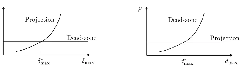
This theorem can be interpreted as stating that if the a-priori knowledge of the paramet-ric uncertainty levelδmaxis sufficiently conservative (δmax≥δmax∗ ), then the dead-zone based
design will out-perform the projection based design, see figure 1(left).
δmax δ∗
max
Projection
Dead-zone
P
dmax d∗max
Dead-zone
Projection
[image:7.612.91.498.501.616.2]P
Figure 1: Statement of the main results: TheoremI (left), TheoremII (right)
Theorem II. Consider the system Σ(x0, θ, d(·)) and the controllers ΞD(·) and ΞP(·)
there exists δ > 0 such that for all δmax ≥ δ, there exists d∗max ≥ ǫ > 0 such that for all dmax≥d∗
max,
P(Σ (X0(γ),Λ,D(ǫ)),ΞD(dmax))>P(Σ (X0(γ),Λ,D(ǫ)),ΞP(δmax)),
wherePis the transient performance cost functional(17),Λ⊂∆(δ)is compact andΛ6⊂∆(0).
This theorem can be interpreted as stating that above a certain uncertainty levelδ, if the a-priori knowledge dmax of the disturbance level is sufficiently conservative (dmax≥d∗max),
then the projection design will out-perform the dead-zone design, see figure 1 (right).
As an aside, we observe that it is natural to ask whether there is any benefit of adaptive control when a boundδmaxis known, as with this information, the natural static output feed-backu(t) =−δmaxy(t) achieves stabilization. One scenario in which adaptive strategies can
be shown to outperform such memoryless feedbacks is when δmax is a conservative estimate
for δ, see, e.g. [F] for such an argument in a related context. In the context of this paper, similar arguments also show that one should utilize dead-zone adaptive controllers in prefer-ence to memoryless feedbacks in the scenario whereby δmax is a conservative estimate forδ,
and dmax is small. In the scenario where dmax is a conservative bound on ǫ, the motivation for adaptation e.g. using the projection design over the memoryless design is less clear-cut. However, if bothδmaxanddmaxare conservative estimates ofδ andǫrespectively, and classes
of disturbances are considered in which adaptive law does not drift, (as for example in the disturbance free case), the projection design will in general not cause ˆδto reach the projection valueδmax, and hence can be expected to generate a lower cost than the high gain memoryless
design.
5. Proof of Theorem I
Firstly, we show that P = ∞ for the unmodified design (11), (Proposition 5.3). From this we can show that the projection modification design, ΞP(δmax) has the property that P → ∞ asδmax → ∞ (Proposition 5.4). Finally we show that P <∞, and that the bound
is independent of δmax, for the dead-zone design, ΞD(dmax) (Proposition 5.5). This suffices
to establish Theorem I.
Proposition 5.1. Consider the closed loop system (Σ(x0, θ, d(·)),Ξ) defined by (2), (11),
where x0∈Rn, θ∈ S. Let d(·)≡ǫfor some ǫ6= 0. Then
kx(t)k →0 ast→ ∞ ⇐⇒ˆδ(t)→ ∞ast→ ∞.
Proof. Let (xT,ˆδ)T denote the unique global solution [WB] of the closed loop (Σ(x0, θ, d(·)),Ξ) given by equations (2), (11).
→) Suppose for a contradiction that ˆδ(t)6→ ∞. Then ˆδ(t)→δˆ∗ <
∞, since ˆδ(·) is mono-tonically increasing by (11). Therefore since by assumptionx →0 and since the r.h.s. of (2),(11) is continuous, it follows that (x(·),δˆ(·))≡(0,δˆ∗) is an equilibrium point of
the closed loop (Σ(x0, θ, d(·)),Ξ). Hence (x(·),ˆδ(·))≡(0,δˆ∗) must be a solution of the
following equations:
x2(t)−an−1x1(t) +bn−1(ǫ−δˆ(t)x1(t)) = 0,
.. .
But b0 6= 0 since the system is minimum phase. We also have ǫ 6= 0. Therefore
(x(·),δˆ(·))≡(0,δˆ∗) cannot be a solution of (20), hence contradiction. ←) Letζ >0 and recalling that y=Cx,z=N x, define
V(t) = 1 2y(t)
2+z(t)TRz(t), t
≥0,
whereRis defined by equation 8. The time derivative ofV along the solution of (7),(11) is
˙
V(t) =y(t)(¯a1−bn−1δˆ(t))y(t) + ¯A2z(t) +bn−1ǫ
+ 2y(t) ¯AT3Rz(t) +z(t)T( ¯AT4R+RA¯4)z(t)
=−(bn−1δˆ(t)−¯a1)y(t)2+ bn−1
√ ζ y(t)·
p
ζ ǫ+y(t) ¯A2+ 2 ¯AT3R
z(t)− kz(t)k2
≤ −(bn−1δˆ(t)−M)y(t)2−1
2kz(t)k
2
+1 2ζ ǫ
2,
whereM :=|¯a1|+
b2
n−1
2ζ + kA¯2k+ 2kRk kA¯3k
2
/2. We choosetζ >0 such thatbn−1δˆ(t)− M >1/2 for allt≥tζ. Therefore
˙
V(t)≤ −αV(t) +1 2ζ ǫ
2 ∀t≥t
ζ,
whereα= min{1,1/2λ(R)}. It follows that
lim
t→∞supV(t)≤ ζ ǫ2
2α .
Since ζ is arbitrary, this proves limt→∞V(t) = 0, hence limt→∞(y(t), z(t)T) = 0. This
completes the proof.
Proposition 5.2. Consider the closed loop system (Σ(x0, θ, d(·)),Ξ) defined by (2), (11),
where x0∈Rn, θ∈ S. Let d(·)≡ǫfor some ǫ6= 0. If x(·) is uniformly continuous, then
kx(t)k →0, δˆ(t)→ ∞ ast→ ∞.
Proof. Let (xT,ˆδ)T denote the unique global solution [WB] of the closed loop (Σ(x
0, θ, d(·)),Ξ)
given by equations (2), (11), and recall thaty =Cx,z=N x. Firstly we show thaty(t)→0 ast→ ∞. From this we will prove that ˆδ(t)→ ∞and finally by Proposition 5.1, we conclude thatkx(t)k →0 as t→ ∞.
Suppose for a contradiction that y(t) 6→ 0 as t → ∞. Then there exists M > 0 and a positive sequence {tk}k≥1 , tk → ∞ as t→ ∞ for which y(tk) ≥M. Since, by assumption,
x(·) is uniformly continuous, it follows that y(·) is uniformly continuous, and hence
∃ω >0 s.t.∀τ ∈[0, ω], and ∀t >0, |y(t)−y(t+τ)|< M
2 . (21)
Therefore|y(tk)−y(tk+τ)|< M/2 and sincey(tk)≥M, we have that y(tk+τ)> M/2 i.e.
y(t)≥M/2 for all t∈[tk, tk+ω]. Without loss of generality, we may assumetk+1−tk≥ω.
It follows that ˆ
δ(tk+ω) =
Z tk+ω
0
˙ˆ
δ(τ)dτ = Z tk+ω
0
y2(τ)dτ ≥ M 2
so ˆδ(tk+ω) → ∞ask → ∞, hence ˆδ(t) → ∞as t→ ∞. It follows by Proposition 5.1 that
kx(t)k →0 as t→ ∞, therefore y(t)→0 ast→ ∞ by (2), hence contradiction.
Now we have y(t) =x1(t)→0 as t→ ∞ and we claim ˆδ(t)→ ∞ ast→ ∞. Suppose for
contradiction ˆδ(t) 6→ ∞ ast→ ∞. Then ˆδ(t)→ δˆ∗ <
∞ ast→ ∞, since ˆδ(·) is monotonic by (11). Substitute this into (2), we have
˙
x1(t) = x2(t)−(an−1+ ˆδ∗bn−1)x1(t) +bn−1ǫ, (23)
.. . ˙
xn(t) = −(a0+ ˆδ∗b0)x1(t) +b0ǫ, (24)
where by minimum phase assumption, biǫ 6= 0, i ∈ [0, n−1]. Since x1(t) → 0 as t → ∞,
equation (24) implies thatxn(t)→ ∞ast→ ∞, sincex(·) is uniformly continuous. It follows
that xn−1(t) → ∞ as t→ ∞, and cascading the argument shows tox1(t) → ∞ ast → ∞,
hence contradiction. Therefore ˆδ(t) → ∞ as t → ∞. From this and Proposition 5.1, the claim of the Proposition follows.
Proposition 5.3. Consider the closed loop system (Σ(x0, θ, d(·)),Ξ) defined by (2), (11), where x0 ∈ Rn, θ ∈ S, d ∈ L∞. Let δ, ǫ, γ > 0 and suppose ∅ 6= Λ ⊂ ∆(δ) is compact.
Consider the transient performance cost functional (17). Then
P( Σ (X0(γ),Λ,D(ǫ)),Ξ) =∞. (25)
Proof. Let lim denote lim sup
t→∞
. Let x0 ∈ X0(γ) and θ∈ Λ. Letd1(·) ≡ǫ6= 0, and consider
(Σ(x0, θ, d1),Ξ). Consider the two cases: either 1. limkx˙(t)k=∞ or 2. limkx˙(t)k<∞:
1. Suppose limkx˙(t)k=∞, i.e. limkAx(t) +Bu(t) +Bǫk=∞. Therefore either
(a) limkx(t)k=∞, which implies that kx(·)kL∞ =∞, or
(b) limkx(t)k<∞, therefore lim u(t) =∞ i.e. ku(·)kL∞ =∞.
2. Suppose limkx˙(t)k<∞i.e. x(·) is uniformly continuous. Therefore by Proposition 5.2
∀δˆ∗ >0 ∃T >0 s.t. ∀t > T δˆ(t)>δˆ∗. (26)
Now we choose d2(t) :=ǫ, ∀t≤T,d2(t) :=−ǫ, for all t > T. Note that d2(t) =d1(t) for all t ≤ T and d2 ∈ D(ǫ). Consider (Σ(x0, θ, d2),Ξ). With this choice, and by
continuity and causality, we have that
lim
t→T+x(t) =x(T), t→limT+ ˆ
δ(t) = ˆδ(T) (27)
where limt→T+ denote limt→T,t>T. It follows that
lim
t→T+u˙(t)
−u˙(T) = 2ˆδ(T)CBǫ≥2ˆδ∗bn−1ǫ. (28)
By choosing a suitable ˆδ∗, it follows that ˆδ(T) can be made arbitrarily large and hence
the difference (28) is arbitrarily large. Then either ˙u(T) is large or limt→T+u˙(t) is large, therefore ku˙(·)kL∞ can be made arbitrarily large.
Therefore at least one component of (17) is unbounded, hence
Proposition 5.4. Consider the closed loop system (Σ(x0, θ, d(·)),ΞP(δmax)) defined by (2),
(16), where x0 ∈Rn, θ ∈ S, d∈ L∞. Let δ, ǫ, γ >0 and suppose ∅ 6= Λ ⊂∆(δ) is compact.
Consider the transient performance cost functional (17). Then
P(Σ (X0(γ),Λ,D(ǫ)),ΞP(δmax))→ ∞ as δmax→ ∞.
Proof. Let M > 0. By Proposition 5.3 there exists x0 ∈ X0(γ), d(·) ∈ D(ǫ), θ ∈Λ so that
the closed loop (Σ(x0, θ, d(·)),Ξ) satisfies
kx(·)kL∞
[0,∞)+ku(·)kL∞
[0,∞)+ku˙(·)kL∞
[0,∞)≥2M.
It follows that ∃T > 0 s.t. kx(·)kL∞
[0,T]+ku(·)kL∞
[0,T]+ku˙(·)kL∞
[0,T] ≥ M. By
choos-ing δmax = 2ˆδ(T), we have that δmax > δˆ(T), hence the solutions (Σ(x0, θ, d(·)),Ξ) and (Σ(x0, θ, d(·)),ΞP(θmax)) are identical on [0, T], and therefore
P(Σ (X0(γ),Λ,D(ǫ)),ΞP(δmax))≥ kx(·)kL∞
[0,T]+ku(·)kL∞
[0,T]+ku˙(·)kL∞
[0,T]≥M.
Since this holds for allM >0, this completes the proof.
Proposition 5.5. Consider the closed loop (Σ(x0, θ, d(·)),ΞD(dmax)) defined by (2), (14),
where x0 ∈ Rn, θ ∈ S, d ∈ L∞. Let δ, ǫ, γ > 0 and suppose ∅ 6= Λ ⊂ ∆(δ) is compact.
Consider the transient performance cost functional (17). Then
P(Σ (X0(γ),Λ,D(ǫ)),ΞD(dmax))<∞, ∀dmax> ǫ≥0. (29)
Proof. Letx0 ∈ X0(γ), θ∈Λ andd∈ D(ǫ). A direct application of Property D2 of Theorem
3.1 guarantees the boundedness ofx(·),δˆ(·), u(·) as a continuous function ofx0, θ, dmax. Since
˙
u(t) =−y(t)2Ddmax(y(t))−δˆ(t)C
A−δˆ(t)BCx(t) +Bd(t), ∀t≥0
it follows thatku(·)kL∞ is bounded in terms of a continuous function ofx0, θ, dmax. Therefore
P(Σ(x0, θ, d(·)),ΞD(dmax))≤M(x0, θ, dmax),
for some continuous function M :Rn× S ×R≥0 →R≥0. Taking the supremum over system
parameters x0, θ, d implies that for all dmax≥ǫ,
P(Σ (X0(γ),Λ,D(ǫ)),ΞD(dmax))≤ sup
x0∈X0(γ) sup
θ∈Λ
sup
d∈D(ǫ)
M(x0, θ, dmax)<∞.
Proof of Theorem I.
This is a simple consequence of Proposition 5.4 and Proposition 5.5.
6. Proof of Theorem II
In order to prove Theorem II, we first give the following Propositions:
Proposition 6.1. Consider the closed loop system (Σ(x0, θ, d(·)),ΞD(dmax)) defined by (2),
(14), where x0 ∈Rn, θ ∈ S, d∈ L∞. Let δ, ǫ, γ >0 and suppose ∅ 6= Λ ⊂∆(δ) is compact,
and Λ 6⊂∆(0). Consider the transient performance cost functional (17). Then ∃δ >0 such that
Proof. Since Λ 6⊂ ∆(0), there exists θ ∈ Λ such that A has an eigenvalue with strictly positive real part or a purely imaginary eigenvalue. In either case it follows that there exists
x0 ∈ X0(γ)∩[−η , η] andd∈ D(ǫ) such that lim sup
t→∞ |
˜
x(t)|=∞ where ˜x(·) is the solution to:
˙˜
x(t) =Ax˜(t) +Bd(t) x˜(0) =x0 t∈[0,∞).
Consider the closed loop system (Σ(x0, θ, d(·)),ΞD(dmax)) and defineτ as follows:
τ = (
∞ ify(t)∈[−η , η] ∀t≥0 inf{t≥0| |y(t)| ≥η}, otherwise.
Note that by dead-zone definition (14), δ˙ˆ(t) = 0 for all t ∈ [0, τ), hence ˆδ(t) = 0 for all
t∈[0, τ) since ˆδ(0) = 0. Therefore
˙
x(t) =Ax(t) +Bd(t) x(0) =x0 ∀t∈[0, τ).
Since x(t) = ˜x(t) fort∈[0, τ) it follows by the observability of (A, C) thaty(t) =Cx(t) hits the boundary of [−η , η] in finite time, i.e. τ <∞. It follows that
kx(·)kL∞ ≥ |y(τ)|=η=dmax.
Hence P(Σ(x0, θ, d(·)),ΞD(dmax))→ ∞ asdmax→ ∞, and therefore
P(Σ (X0(γ),Λ,D(ǫ)),ΞD(dmax)) → ∞ asdmax→ ∞.
Proposition 6.2. Consider the closed loop(Σ(x0, θ, d(·)),ΞP(δmax))defined by(2),(16),where x0 ∈Rn, θ∈ S, d∈ L∞. Let δ, ǫ, γ >0 and suppose ∅ 6= Λ⊂∆(δ) is compact. Then for all δmax≥δ,
P(Σ (X0(γ),Λ,D(ǫ)),ΞP(δmax))<∞. (30)
Proof. Let x0 ∈ X0(γ),θ∈Λ, d∈ D(ǫ). A direct application P2 of Theorem 3.2 guarantees
the boundedness of signals x(·),δˆ(·), u(·) of the closed loop (Σ(x0, θ, d(·)),ΞP(δmax)) as a
continuous function of x0, θ,kdk, δmax. It follows that
˙
u(t) =−y(t)3−δˆ(t)C(Ax(t) +B(u(t) +d(t)))
is bounded in terms of a continuous function of x0, θ,kdk, δmax, hence
P(Σ(x0, θ, d(·)),ΞP(δmax))≤M(x0, θ, δmax,kdk)<∞, (31)
whereM :Rn×V ×R≥0 →R≥0is continuous. Taking the supremum over system parameters x0, θ, d implies that for all δmax≥δ
P(Σ (X0(γ),Λ,D(ǫ)),ΞP(δmax))≤ sup
x0∈X0(γ) sup
θ∈Λ
sup
d∈D(ǫ)
M(x0, θ, δmax,kdk)<∞.
Proof of Theorem II.
This is a simple consequence of Proposition 6.2 and Proposition 6.1.
The proof of Theorem II is heavily based on the natural assumption that the size of dead-zone η is chosen to be equal to the a-priori bound on the disturbance level dmax. In
particular, η := dmax implies that P(Σ (X0(γ),∆(δ),D(ǫ)),ΞD(dmax)) → ∞ as dmax → ∞.
7. Alternative Choices of Dead-zones
In this section we consider alternative choices for the dead-zone, and variations on the definition of the controller. We consider the following smooth dead-zone controller (compare to equation (14)):
ΞD,̺(dmax) : u(t) =−δˆ(t)y(t))
˙ˆ
δ(t) =|y(t)|Dη(y(t)), δˆ(0) = 0, η:=̺(dmax)
(32)
where̺: [0,∞)→[0,∞), noting that we have previously considered the case where̺(r) =r. We consider two possibilities for the growth of the function̺:1
(i) limr→∞̺(r) =∞,
(ii) limr→∞̺(r)≤c for some constantc≥0.
In case (i) it is straightforward to observe that
P :=P(Σ (X0(γ),Λ,D(ǫ)),ΞD,̺(dmax))→ ∞ asdmax→ ∞, (33)
by the same argument as in Proposition 6.1.
Choice (ii) is also a viable option, since ΞD,̺(dmax) = ΞD(̺(dmax)), and by Theorem 3.1, P(Σ (X0(γ),Λ,D(ǫ)),ΞD,̺(dmax))<∞and limt→∞ infx∈[−̺(dmax),̺(dmax)]|y(t)−x|= 0.This choice has been extensively studied in the context of tracking, where the case ̺(r) = λ is known as λ–tracking [IR]. The next result shows that ifc is too small, then the projection controller out-performs the dead-zone design. For simplicity we consider a scalar system:
Proposition 7.1. Consider the system Σ(x0,(a,1), d(·)) and the controllers ΞD,̺(·) and
ΞP(·) defined by(2), (32) and (16) respectively, where x0 ∈ R, a ∈ R, d ∈ L∞ and where
limr→∞̺(r) ≤c for c > 0. Let δ, ǫ >0 and let Λ ={(a,1)∈ R2 : |a| ≤δ}. Consider the
transient performance cost functional(17). Then for all dmax≥ǫ, and for allδmax≥δ, there
exists c∗ >0 such that for all 0< c < c∗,
P(Σ (X0(γ),Λ,D(ǫ)),ΞD,̺(dmax))>P( Σ (X0(γ),Λ,D(ǫ)),ΞP(θmax) ).
Proof. Let x0 ∈ X0(γ) and suppose (a,1) ∈ Λ is such that a > 0. Let d(·) = ǫ > 0 be
constant. Consider (Σ(x0,(a,1), d),ΞD,̺(dmax)). Sincey(t)→[−̺(dmax), ̺(dmax)] as t→ ∞,
there existsT >0 such thaty(T)≤2̺(dmax) and 12dtdy(T)2= ˙y(T)y(T)≤0. It follows that,
(ˆδ(T)−a)≥ ǫ 2̺(dmax)
.
Define d2(·) as in Proposition 5.3 and consider (Σ(x0, θ, d2),ΞD,̺(dmax)). It follows that
lim
t→T+u˙(t)
−u˙(T) = 2ˆδ(T)ǫ= ǫ
2
̺(dmax) ≥ ǫ2
c.
Hence for allP∗ >0, there existsc∗ >0 such that for all 0< c < c∗, P(Σ (X0(γ),Λ,D(ǫ)),ΞD,̺(dmax)) = sup
x0∈X0(γ) sup
θ∈Λ
sup
d∈D(ǫk)
˙
u(·)kL∞,
> P∗. (34)
The proof is completed by choosingP∗ =
P( Σ (X0(γ),Λ,D(ǫ)),ΞP(θmax) )<∞.
1
Similar results can be obtained in the tracking setting, where the error signal e(·) =
y(·)−yref(·) replaces the statex(·) =y(·) and ˙yref(·)−θyref(·) plays an analogous role to the
disturbanced(·). See [S], [SF] for further discussions.
8. Conclusion
In this paper we have established two rigorous results to demonstrate situations in which we can compare the transient performance of projection and dead-zone based controllers of non identifier based adaptive designs. We have shown that
• The dead-zone based controller outperforms the projection based controller when the a-priori information on the uncertainty level is sufficiently conservative.
• The projection based controller outperforms the dead-zone based controller when the a-priori information on the disturbance level is sufficiently conservative.
Our results are based on the a-priori information dmax and θmax. We have also shown
that other choices of controllers with differing dependence on a-priori information such as
λ–tracking controllers can be driven to similar conclusions.
There are a number of directions in which the result can be generalised, for example: (i) generalisation of the result for adaptive controllers for higher relative degree plants, (ii) generalisation of the results for nonlinear systems in the form of integrator chain [S], or in the strict feedback form, and (iii) establishing whether the same results can be given for the alternative costs, for example,P =kx(·)kL∞+ku(·)kL∞.
It would also be of interest to determine explicit tight bounds ond∗
max, δ∗max, note however
that this is challenging as it would require tight upper and lower bounds on performance of both controllers.
Acknowledgements. We would like to express our gratitude to the reviewers for their perceptive comments and detailed reading of the draft manuscript.
Appendices
The proofs of Theorems 3.1 and 3.2 are given in this part.
Appendix A. Proof of Theorem 3.1
Before we give the proof, we first present a preliminary Lemma:
Lemma A-1. Suppose M ∈Rn×n, n≥1is an stable matrix. Let the positive definite matrix
G∈Rn×n be the solution of the Lyapunov equation
GM+MTG=−I.
Then for all t≥0,
keM tk ≤k1e−kt, k:= 1/λ(G), k1:= q
λ(G)/λ(G),
Proof. The proof is elementary and omitted for brevity.
The proof of Theorem 3.1 is derived from the technique used in the proof of ‘λ–tracking’ based on [I2](pages 112–117) but with a significant extension to obtain property D2.
Proof of Theorem 3.1. The continuity ofDηimplies by classical result of differential
equa-tions that there exists a unique solution (x(·),ˆδ(·)) over a maximal interval of existence [0, ω) for someω∈(0,∞]. Using the transformation defined by (5), we obtain
˙
y(t) = ¯a1−bn−1δˆ(t)
y(t) + ¯A2z(t) +bn−1d(t), y(0) =Cx0, (A-1)
˙
z(t) = A¯3y(t) + ¯A4z(t), z(0) =N x0, (A-2)
˙ˆ
δ(t) = |y(t)|Ddmax(y(t)), δˆ(0) = 0 (A-3)
Define the C1 function
V(y) :=
0, y∈[−η , η],
1
2(|y| −η)
2, y6∈[−η , η], (A-4)
whereη =dmax≥0. Observe that
˙
V(y(t)) =ζ(t) ˙y(t) ∀t∈[0, ω), (A-5)
where the continuous functionζ : [0, ω)→Ris
ζ(t) :=
0, y(t)∈[−η , η].
(|y(t)| −η) y(t)
|y(t)|, y(t)6∈[−η , η].
(A-6)
Note that by (14)
˙ˆ
δ(t) =ζ(t)y(t) =|ζ(t)| |y(t)|, ∀t∈[0, ω) (A-7)
and by the continuity of (A-6),|y(t)| |ζ(t)| ≥η|ζ(t)|, or
|ζ(t)| ≤η−1|ζ(t)| |y(t)|=η−1δ˙ˆ(t), ∀t∈[0, ω) (A-8)
Substituting (A-1) in (A-5), we have for allt∈[0, ω),
˙
V(y(t)) = (¯a1−bn−1δˆ(t))y(t)ζ(t) + ¯A2z(t)ζ(t) +bn−1d(t)ζ(t)
≤ (¯a1−bn−1δˆ(t))δ˙ˆ(t) +bn−1kd(·)kL∞|ζ(t)|+kA2¯ k kz(t)k |ζ(t)|
≤ (M1−bn−1δˆ(t))δ˙ˆ(t) +kA¯2k kz(t)k |ζ(t)|, (A-9)
where M1 := M1(θ, dmax,kd(·)kL∞) := |¯a1|+η−1bn−1kd(·)kL∞. Note that the continuous
dependency of M1 on θ ∈ S follows from definition (4) and transformation (6) which also
depends continuously onθ∈ S. M1 also depends continuously on dmax by definition (14). Now we derive a relation between the second part of (A-9) and ˆδ(·). Rewrite equation (A-2) as
˙
z(t) = ¯A4z(t) + ¯A3ζ(t) +h(t), (A-10)
where
Note that since
y−ζ =
y, |y|< η
η y
|y|, |y| ≥η
we have that|h(t)| ≤ηkA¯3k. Since ¯A4is exponentially stable, by Lemma A-1, for allt∈[0, ω)
M2e−µt≥ keA¯4tk, M2 :=M2(θ) = s
λ(R)
λ(R), µ:=µ(θ) = 1/λ(R), (A-11)
where R is defined in (8). M2 and µ depend continuously on θ ∈ S since ¯A4 depends
continuously on θ ∈ S, hence R and its eigenvalues are continuously dependent on θ ∈ S. Therefore by equation (A-10), we have for allt∈[0, ω)
kz(t)k ≤ M2e−µtkz0k+M2 Z t
0
e−µ(t−s)(kA¯3k |ζ(s)|+|h(s)|)ds
≤ M2e−µtkz0k+M2kA3¯ k
Z t
0
e−µ(t−s)|ζ(s)|ds+M2kA3¯ kηµ−1(1−e−µt)
≤ M3
1 + Z t
0
e−µ(t−s)|ζ(s)|ds
, (A-12)
where M3 := M3(x0, θ) := M2kz0k+kA¯3k(1 +ηµ−1). The continuous dependency of M3
on x0, θ ∈ S, dmax follows from the definition of η and the continuous dependency of S−1,µ
and M2 on θ∈ S. Lett∈[0, ω). From inequality (A-12) it follows that
Z t
0 k
z(s)k |ζ(s)|ds≤M3 Z t
0 |
ζ(s)|+M3 Z t
0 | ζ(s)|
Z s
0
e−µ(s−τ)|ζ(τ)|dτ ds. (A-13)
Using the Cauchy-Schwarz inequality, we have that
Z t
0| ζ(s)|
Z s
0
e−µ(s−τ)|ζ(τ)|dτ ds≤ kζ(·)kL2(0, t)· Z • 0
e−µ(•−τ)|ζ(τ)|dτ L2(0, t)
.
An application of the following inequality (Theorem 6.5.54)[V]
Z • 0
e−µ(•−τ)|ζ(τ)|dτ
L2(0, t)≤ e
−µ•
L1(0, t)· kζ(·)kL2(0, t)≤µ−1kζ(·)kL2(0, t), (A-14)
together with relations (A-13),(A-8) and (A-14), implies
Z t
0 k
z(s)k |ζ(s)|ds ≤ M3(1 +µ−1) Z t
0 |
ζ(s)|+ζ(s)2ds
≤ M3(1 +µ−1) Z t
0
(1 +η−1)|ζ(s)| |y(s)|ds
≤ M4δˆ(t), (A-15)
where M4 := M4(x0, θ) := M3(1 +µ−1)(1 +η−1). Now, using (A-15), we can calculate a
bound onV(y(t)) in terms of ˆδ(t) by integrating (A-9) over [0, t]
V(y(t))≤V(y(0)) + Z t
0
M1−bn−1ˆδ(s)
˙ˆ
δ(s)ds +kA¯2kM4δˆ(t)
≤V0+M5δˆ(t)− bn−1
2 ˆδ(t)
where V0 := V(y(0)), and M5 := M5(x0, θ, dmax,kd(·)kL∞) :=M1+kA¯2kM4. The positive
definiteness ofV implies that
−bn2−1δˆ(t)2+M5δˆ(t) +V0 ≥0. (A-16)
Solving the quadratic inequality (A-16) for ˆδ(t), we have that
M5−M6 bn−1 ≤
ˆ
δ(t)≤ M5+M6
bn−1
, (A-17)
where M6 := M6(x0, θ, dmax,kd(·)kL∞) := p
M52+ 2bn−1V0 > M5. We discard the non–
positive lower bound of (A-17) due to the fact that by (A-3), ˆδ(0) = 0 and ˆδ(·) is non decreasing. Therefore
0≤δˆ(t)≤ M5+M6 bn−1
. (A-18)
The continuous dependency on x0, θ, dmax of M4–M6 is a consequence of the continuous
dependency of M3, µ and the coordinate transformation (6). We now define a continuous function V∗ :
Rn× S ×R≥0 ×R>0 → R≥0 by V∗(x0, θ,kd(·)kL∞, dmax) = V0 +M5(M5 + M6)/bn−1. Then
V(y(t))≤V∗(x0, θ,kd(·)kL∞, dmax) ∀t∈[0, ω), (A-19)
The boundedness ofy(·) in terms ofV∗(x
0, θ,kd(·)kL∞, dmax) on [0, ω) follows from 4),
(A-19). Therefore by (A-6),ζ(·) is bounded by a continuous function ofV∗(x
0, θ,kd(·)kL∞, dmax)
on [0, ω). Hence by (A-12),z(·) is bounded by a continuous function ofV∗(x
0, θ,kd(·)kL∞, dmax)
on [0, ω). It follows by (6) that x(·) ∈ L∞(0, ω) is bounded by a continuous function of V∗(x
0, θ,kd(·)kL∞, dmax). The continuity of the right hand side of equations (A-1)–(A-3) and
the boundedness of the solution (x(·),δˆ(·)) implies that ω =∞. Finally the boundedness of
u(·) as a continuous function ofV∗(x
0, θ,kd(·)kL∞, dmax) follows from (14), thus establishing
D1–D2.
Since y(·) is bounded, it follows from the definition of ˆδ(·) that δ˙ˆ(·) is uniformly con-tinuous. Furthermore, δ˙ˆ(·) ∈ L1, hence Barbalat’s lemma shows δ˙ˆ(t) → 0 as t → ∞. So
limt→∞infx∈[−η,η]|y(t)−x|= 0 hence proving D3, and thus completing the proof.
Appendix B. Proof of Theorem 3.2
Proof of Theorem 3.2. Since the (time-varying) right hand side of the differential equa-tions (2) and (16) is piecewise locally Lipschitz, a unique piecewise absolutely continuous local solution exists. Let (x(·),ˆδ(·)) denote a solution of closed loop (Σ(x0, θ, d(·)),ΞP(δmax))
on a maximum interval of existence [0, ω) for some ω ∈ [0,∞). Using the transformation defined by (5), we obtain
˙
y(t) = ¯a1−bn−1δˆ(t)
y(t) + ¯A2z(t) +bn−1d(t), y(0) =Cx0, (B-1)
˙
z(t) = A¯3y(t) + ¯A4z(t), z(0) =N x0, (B-2)
˙ˆ
δ(t) = (
y(t)2 δˆ(t)< δmax
0 δˆ(t)≥δmax
By definition of projection modification (16), ˆδ(t) ≤δmax for all t≥0. Let k∗θ < δmax be
given by equation (10). The monotonicity of ˆδ(·) implies that either (i) ˆδ(t) < k∗
θ for all
t∈[0, ω), or (ii) there existst∗∈[0, ω) such that ˆδ(t)≥k∗
θ for all t∈[t∗, ω).
(i) If ˆδ(t) < kθ∗ for all t ∈ [0, ω) then by (16) we have δ˙ˆ(t) = y(t)2 for all t ∈ [0, ω). It
follows that Z ω
0
y(s)2ds < kθ∗,
and hence y(·) ∈ L2[0, ω). Since ¯A
4 is stable, (B-2) can be considered as anL2 input y(·) to a stable system ˙z(t) = ¯A4z(t) + ¯A3y(t) for all 0≤t < ω, from which follows that
˙
z(·), z(·) ∈ L2[0, ω). An explicit bound on kzk L2
[0,ω) can be obtained as follows. Note
that since y(·) ∈ L2[0, ω) and ¯A
4 is exponentially stable, by Lemma A-1, there exists M0, ν ≥0 such that for all t∈[0, ω)
M0e−νt≥ ke ¯
A4t
k M0 :=M0(θ) = q
λ(R)/λ(R), ν:=ν(θ) = 1/λ(R), (B-4)
whereR is defined in (8). Therefore2
kzkL2[0,ω)≤ keA¯4•z0kL2[0,ω)+k(sI−A¯4)−1A¯3k
H∞kykL2[0,ω) ≤ M0
ν kz0k+k(sI−A¯4) −1A¯
3kH∞ q
k∗
θ.
(B-5)
A bound on z(·) is also required to show the boundedness of x(·). Applying (B-4) to the solution of (A-2), we have that for allt∈[0, ω),
kz(t)k ≤ M0
ν kz0k+M0 Z t
0
e−ν(t−s)kA3¯ k |y(s)|ds
≤M1
1 + Z t
0
e−ν(t−s)|y(s)|ds
,
(B-6)
whereM1:=M1(kx0k, θ) :=M0(ν1kz0k+kA¯3k). Sincey(·)∈ L2[0, ω), andkykL2[0,ω)≤
k∗
θ, it follows that z(·) is bounded as a continuous function of kx0k and θ. It remains
to show y(·) ∈ L∞[0, ω), and to construct an explicit uniform bound for y(
·) which is continuously dependent onx0, θ,kdk, δmax. To this end, consider (A-1) and define:
V1(t) :=
1 2y(t)
2, ∀t∈[0, ω). (B-7)
The time derivative of (B-7) along the solution of (B-1)– (B-3) is bounded by:
˙
V1(t) = (¯a1−bn−1δˆ(t))y(t)2+ ¯A2z(t)y(t) +bn−1d(t)y(t)
= −1 2y(t)
2+ (¯a
1+ 1)y(t)2−bn−1δˆ(t)y(t)2+ ¯A2z(t)y(t)−
1 2y(t)
2+b
n−1d(t)y(t)
≤ −V1(t) + (¯a1+ 1 +kA¯2k2)y(t)2+|z(t)|2+ b2n−1
2 kd(·)k
2
L∞, ∀t∈[0, ω) (B-8)
2
Recall thatkG(·)kH∞ = ess sup
ω∈R
where (B-8) follows from two applications of Young’s inequality and by observing that
bn−1ˆδ(t)>0 for allt∈[0, ω). Hence for all t∈[0, ω),
1 2y(t)
2 ≤ V 1(t)
≤ e−tV1(0) + Z t
0
e−(t−s)((¯a1+ 1 +kA2¯ k2)y(s)2+|z(s)|2+ b
2
n−1
2 kd(·)k
2 L∞) ds
≤ y(0) 2
2 + (¯a1+ 1 +kA¯2k
2
)ky(·)k2L2[0,ω)+kz(·)k2L2[0,ω)+
b2n−1
2 kd(·)k
2
L∞.(B-9)
Sinceky(·)k2
L2[0,ω)< kθ∗ which is continuously dependent onθ, and we have shown that
kz(·)k2
L2[0,ω) is bounded as a continuous function of |x0| and θ, it follows that y(·) is bounded on [0, ω) in terms of a continuous function ofx0, θ,kdkandδmax. It follows by
(B-6) and (6) thatx(·) is bounded on [0, ω) as a continuous function ofx0, θ,kdk, δmax.
(ii) Suppose there exists t∗
∈ [0, ω) such that ˆδ(t) ≥ k∗
θ for all t ∈ [t
∗, ω). Define the
Lyapunov function
V2(t) = ¯x(t)TPx¯(t), ∀t∈[0, ω) (B-10)
where ¯x(t), P are defined by (6) and (9) respectively.
Then allt∈[0, ω), the time derivative of V2(t) w.r.t. (B-1)– (B-3) is given by:
˙
V2(t) =¯x(t)TPx˙¯(t) + ˙¯x(t)TPx¯(t),
=¯x(t)TPD¯(ˆδ(t))¯x(t) + ¯Bd(t)+D¯(ˆδ(t))¯x+ ¯Bd(t)TPx¯(t),
=¯x(t)TPD¯(ˆδ(t)) + ¯DT(ˆδ(t))Px¯(t) + 2¯x(t)TPBd¯ (t),
(B-11)
whereS is given by (5) and ¯B :=S−1B, ¯D(•) :=S−1(A− •BC)S. Let
µ(θ,kdk) := 2 p
λ(P)
λ(Q) |PB¯| kd(·)kL∞,
whereQis defined in (9). Thenµis continuously dependent onθ∈ S by the continuity of the transformation (6). By (9), we observe that
˙
V2(t) ≤ −x¯(t)TQx¯(t) + 2¯x(t)TPBd¯ (t), (B-12)
≤ − λ(Q)−2
p λ(P) p
V2(t)
|PB¯| kd(·)kL∞ !
kx¯(t)k2, (B-13)
≤ −λ(Q) 1−µp(θ,kdk) V2(t)
!
kx¯(t)k2, ∀t∈[t∗, ω). (B-14)
Inequality (B-14) implies that ˙V2(t)<0 for allV2(t)> µ(θ,kdk)2, i.e.
V(t)≤V′(¯x∗, θ,
kdk) := max{V2(¯x∗), µ(θ,kdk)2} ∀t∈[t∗, ω), (B-15)
where ¯x∗ := ¯x(t∗). Therefore, by (B-10), ¯x(·) is bounded on [t∗, ω) in terms of V′(¯x∗, θ,
kdk). A bound on ¯x(·) on [0, t∗) and a bound on the end point ¯x(t∗) as
a continuous function of x0, θ,kdk, δmax follows directly by the argument of part (i)
where ˆδ(t)< k∗
θ < δmaxfor allt∈[0, t∗). Hence by the continuity of the transformation
The boundedness of x(·) over [0, ω) implies that x(·) cannot have a finite escape time. By definition (16), ˆδ(·) is also known never to leave the set [0, δmax]. Hence ω = ∞ i.e. the solution (x(·),δˆ(·) ) exists for all t ∈ [0,∞). Furthermore, the solution is bounded as a continuous function of x0, θ,kdk, δmax. Finally, the boundedness of u(·) as a continuous
function of x0, θ,kdk, δmax follows by (16).
References
[E] B. Egardt. Stability of adaptive controllers. Lecture notes in Control and Informa-tion Sciences, Springer–Verlag, New York, 1979.
[F] M. French. An analytical comparison between the nonsingular quadratic perfor-mance of robust and adaptive backstepping designs. IEEE Trans. on Automatic Control, 47(4):670–675, 2002.
[GI] P. Georgieva and A. Ilchmann. Adaptive λ–tracking control of activated sludge processes. International Journal of Control, 74:1247–1259, 2001.
[I1] A. Ilchmann. Non–Identifier–Based Adaptive Control of Dynamical systems: A Survey. IMA Journal of Mathematical Control and Information,8:321–366, 1991.
[I2] A. Ilchmann. Non–Identifier–Based High–Gain Adaptive Control. Lecture notes in Control and Information Sciences, Springer–Verlag, London, 1993.
[IR] A. Ilchmann and E. P. Ryan. Universal λ-tracking for nonlinearly perturbed sys-tems in the presence of noise. Automatica, 30:337–346, 1994.
[IT] A. Ilchmann and S. Townley. Adaptive sampling control of high-gain stabilizable systems. IEEE Trans. on Automatic Control, 44(10):1961–1966, 1999.
[KKK] M. Kristic, I. Kanellakopoulos, and P. Kokotovic. Nonlinear and Adaptive Control Design. John Wiley & Sons, New York, 1995.
[KN] G. Kreisselmeier and K. S. Narendra. Stable model reference adaptive control in the presence of bounded disturbances. IEEE Trans. on Automatic Control, 27(6):1169–1175, 1982.
[LK] K. W. Lee and H. K. Khalil. Adaptive output feedback control of robot manipula-tors using high-gain observer. Int. Journal of Control, 67(6):869–886, 1997.
[LT] H. Logemann and S. Townley. Adaptive stabilization without identification for distributed parameter systems: An overview. IMA Journal Mathematical Control and Information, 20:175–206, 1997.
[M] B. M˚artensson. The order of any stabilizing regulator is sufficient a priori informa-tion for adaptive stabilizainforma-tion. Systems and Control Letters, 6:87–91, 1985.
[NA] K. S. Narendra and A. M. Annaswamy. Stable Adaptive Systems. Prentice–Hall, 1989.
[R] E. P. Ryan. A universal adaptive stabilizer for class of nonlinear systems. Systems and Control Letters, 16:209–218, 1991.
[S] A. Sanei. Towards a Performance Theory of Robust Adaptive Control. PhD the-sis, Department of Electronics and Computer Science, University of Southampton, U.K., 2002.
[SF] A. Sanei and M. French. Towards a performance theory of robust adaptive control. International Journal of Adaptive Control and Signal Processing, 18:403–421, 2004.
[T] S. Townley. Topological aspects of universal adaptive stabilization. SIAM Journal Control and Optimization, 34:1044–1070, 1996.
[V] M. Vidyasagar. Nonlinear Systems Analysis. Prentice–Hall, 1978.
[W] A. J. Weir. Lebesgue Integration and Measure. Cambridge University Press, 1991.
[WB] J. C. Willems and C. I. Byrnes. Global adaptive stabilization in the absence of information on the sign of the high–frequency gain. In Lecture Notes in control and information science, Springer–Verlag, Berlin, 62:49–57, 1984.