This is a repository copy of Network meta-analysis explained. White Rose Research Online URL for this paper:
http://eprints.whiterose.ac.uk/137044/ Version: Accepted Version
Article:
Dias, Sofia orcid.org/0000-0002-2172-0221 and Caldwell, Deborah (2018) Network meta-analysis explained. Archives of disease in childhood-Fetal and neonatal edition. ISSN 1359-2998
https://doi.org/10.1136/archdischild-2018-315224
[email protected] https://eprints.whiterose.ac.uk/ Reuse
Items deposited in White Rose Research Online are protected by copyright, with all rights reserved unless indicated otherwise. They may be downloaded and/or printed for private study, or other acts as permitted by national copyright laws. The publisher or other rights holders may allow further reproduction and re-use of the full text version. This is indicated by the licence information on the White Rose Research Online record for the item.
Takedown
If you consider content in White Rose Research Online to be in breach of UK law, please notify us by
Network meta-analysis explained
Sofia Dias1,2* and Deborah M Caldwell2
* Corresponding author: [email protected]; phone: +44 (0)1904 321074
1 Centre for Reviews and Dissemination, University of York, Heslington, YO10 5DD, UK
2 Bristol Medical School, University of Bristol, Canynge Hall, 39 Whatley Road, BS9 2PS,
UK
WHAT IS NETWORK META-ANALYSIS?
Healthcare decisions should be based on all relevant evidence.1 Usually this is provided by
randomised controlled trials (RCTs) comparing two or more interventions for a condition
affecting a target population of interest, although other forms of evidence can be considered.1
2 When more than one study is available, meta-analysis can be used to combine multiple
treatment effects and obtain an overall estimate of the effect in the target population. To
assess clinical effectiveness, evidence from RCTs is typically used and relative treatment
effects estimated in individual trials are pooled using methods that preserve within-trial
randomisation. However, for the majority of health conditions, there are more than two
interventions of interest. In such cases, performing multiple pairwise meta-analyses
(comparing interventions two at a time) or lumping every active intervention to be compared
to a “control” is of limited use for decision-making and does not allow for coherent and
transparent decisions. Decisions involving more than 20 interventions are not uncommon.3-6
The number of pairwise comparisons required to make a decision between 3 interventions is
3, with 5 interventions it is 10, with 10 interventions it is 45 and with 41 interventions4 it is
820. Clearly not all comparisons will have been carried out in RCTs but looking at multiple
separate pairwise analyses carried out using different sets of trials makes it impossible to
decide which intervention is best.
Network meta-analysis (NMA), also termed multiple treatment meta-analysis or mixed
treatment comparisons, was developed as an extension of pairwise meta-analysis to allow
comparisons of more than two interventions in a single, coherent analysis of all the relevant
RCTs.7-10 Its main advantages are that it produces consistent estimates of the relative effects
of all interventions compared to every other in a single analysis using both direct and indirect
two arms (i.e. avoiding double counting of patients). This results in greater precision of
treatment effect estimates and the ability to rank all the interventions in a coherent way.8 As
for standard meta-analysis, NMA can be performed for most types of RCT outcomes,
continuous, dichotomous, event rates and from survival models, using an appropriate scale
(mean difference, odds ratio, relative risk, hazard ratio etc).
The underlying idea is very simple: consider three friends, Anne, Ben and Charles. If we
know that Ben is 7cm taller than Anne, and that Charles is 10cm taller than Anne, then we
know that Charles is 3cm taller than Ben, and is therefore the tallest. We can also rank the
friends in terms of who is tallest as 1=Charles, 2=Ben, 3=Anne. So, by taking Anne’s height
as reference and measuring the heights of the others compared to hers, we know how
everyone’s height compares to each other and how to order the friends by height. The only
assumption being made is that the heights we measured are an accurate reflection of the true
heights of the three friends (in other words, that we used a sufficiently accurate measuring
tool). It is easy to see that the same relative heights and ranks would be obtained if one of the
male friends had been the reference, and how the height relationships would extend if more
than three friends had been measured. This is exactly how NMA works, although we also
take the uncertainty (i.e. the sampling error) in the relative effect estimates into account, as is
standard in meta-analysis.
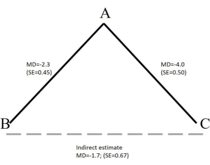
Suppose we are interested in comparing treatments B and C. We find one trial comparing B
to A, giving a mean difference (MD) of -2.3 with a standard error (SE) of 0.45 and one trial
comparing C to A giving a mean difference of -4 with SE 0.5. This suggests that both
treatments B and C are better than A with 95%CIs that exclude no effect: (-3.18, -1.42) for B
compared to A and (-4.98, -3.02) for C compared to A (assuming a reduction in the mean is
absence of a direct RCT, what can we say about the relative effect of treatment C vs B? The
first thing to note is that this question can only be answered in the context of a pre-defined
patient population of interest. That is, one must ensure that the populations included in the
BvsA and the CvsA trials are comparable to each other and to our target population, with
respect to any potential effect modifying characteristics.10 Once it is decided that these
studies were carried out on clinically homogeneous populations (which, in turn, are similar to
the target population) then it can be assumed that each study estimates the true treatment
effects in the target population (i.e. the relative effects were measured using an ‘accurate
measurement tool’). We can therefore say that C is better than B by 1.7 units through the
indirect comparison of treatments C and B,11 since the true treatment effects of BvsA, CvsA
and CvsB must be consistent, ie they must add up in the same way as the friends’ heights. In
other words, the mean difference (MD) of C compared to B must be the difference between
the MDs of CvsA and BvsA, which is -1.7 units. This consistency relationship, sometimes
also called transitivity, must hold if the studies are estimating the true effects in a patient
population. To obtain a 95%CI for the CvsB comparison we simply add the variances of the
two other comparisons to obtain a SE with which a 95%CI can be constructed: (-3.01, -0.39).
This type of comparison is termed ‘indirect’ as it relies on evidence against the comparator A,
and not on ‘direct’ head to head evidence from one or more trials of CvsB.
Suppose now that we also had evidence from a new study on the same patient population
which compared treatment C to B, giving a mean difference of -1.8 95%CI (-3.66, 0.06).
Traditional hierarchies of evidence state that estimates from direct head-to-head RCTs
provide the “best available” evidence of intervention effects. Should we now discard the
indirect evidence? Or perhaps we should prefer the indirect evidence since it suggests a
statistically significant effect? To do either is contrary to the principle of using all relevant
to do a mixed (evidence) treatment comparison, or NMA, under the assumption that both the
direct and indirect evidence are estimating the same, true, underlying treatment effect of
CvsB in our target population. The exact same principles apply when multiple RCTs are
available for each of the possible comparisons and for more than three interventions.
NMA relies on the same assumptions underlying pairwise meta-analysis, that is, that the
included studies are sufficiently homogenous in terms of the condition being studied, the
included participants and the definition of active and control interventions. In other words,
we are assuming that the effects of BvsA and CvsB that would have been observed if the
CvsA RCT had included all three treatments, is the same as that observed in the BvsA RCT
(apart from sample variability). This assumption is the basis for coherent decisions whether
they involve two or more treatments. One way to empirically check this is to ask: “given the
known study and participant characteristics, if all these studies compared the same two
treatments, would it be suitable to combine them in a meta-analysis?”. If the answer to this is
yes, and the only distinction is that instead the studies compare different sets of interventions,
then the assumption of “sufficient homogeneity” is, in principle, satisfied.
Because NMA pools the relative treatment effects estimated across RCTs, within-trial
randomisation is preserved. As long as the interventions of interest form a connected network
of comparisons, then relative effects of each intervention compared to every other can be
obtained, along with estimates of their uncertainty (e.g. 95% confidence intervals). Figure 2
shows two networks of tocolytic interventions compared in a guideline produced for the
National Institute for Health and Care Excellence (NICE)13 which updated a previously
published systematic review and NMA.14 Nine types of tocolytic interventions were of
interest (Table 1) and 98 RCTs were included. To ensure that the assumption of consistency
were first assessed by the reviewers.14 For example, the analysis excluded trials in which
women were at high risk of preterm delivery such as those with multiple gestation and
ruptured membranes. Underpinning this exercise is the need to determine if every individual
included in every trial across the network could have been (hypothetically) randomised to any
of the included treatments. If, for example, a treatment would only be administered to a
multiparous and not nulliparous woman or as a second- or third-line treatment, it is possible
that the assumption of consistency might not hold.
Table 1 Tocolytic therapies of interest
Interventions 1 Placebo/control
2 Prostaglandin inhibitors 3 Magnesium sulfate 4 Betamimetics
5 Calcium channel blockers 6 Nitrates
7 Oxytocin receptor blockers 8 Alcohol/ethanol
9 Other treatments
The first network (Figure 2a) includes 47 RCTs reporting on perinatal death. It is
“connected” as there is a path that connects every treatment and therefore all relative effects
for all interventions compared to every other can be obtained. We can see that the
interventions with the most patients randomised are (in decreasing order) Betamimetics and
Placebo, as they have the widest circles. The second network, Figure 2b), includes the 51
RCTs which reported on estimated gestational age (EGA) at delivery. This figure has two
disconnected interventions: ‘Alcohol/ethanol’ and ‘Other treatments’ cannot be compared to
the rest of the network. For this outcome, comparisons can only be made between the other
characteristics14 15 although the ability to display additional information can be limited by the
size of the network.
NMA MODELS AND ESTIMATING TREATMENT EFFECTS
NMA simultaneously combines the relative treatment effects estimated within each study
whilst accounting for the individual treatments being compared and correctly incorporating
studies with more than two arms. Fixed or random effects models can be fitted, the latter
allows for between-study heterogeneity. NMA random effects models usually assume that the
between-study heterogeneity is the same across all comparisons, that is, a single measure of
heterogeneity is calculated across the whole network, although models allowing for different
heterogeneity for each comparison can also be fitted.16 In the presence of large heterogeneity,
patient or study characteristics that may modify the relative treatment effects (effect
modifying covariates) should be investigated using meta-regression17 or sensitivity analyses.
As a statistical model, NMA can be fitted using a frequentist or Bayesian approach.18 A
Bayesian approach to NMA requires a prior probability distribution to be specified for the
parameter of interest (e.g. treatment effect), describing the range and probability of plausible
values for the parameters, which is combined with a likelihood statement, which describes
the data collected, using Bayes theorem. This produces a posterior distribution which
describes the new range and probability of plausible values for the parameter, on which
statistical inferences are based.19 Uncertainty in the parameters is fully represented by their
posterior distributions, so direct probability statements can be made on e.g. the probability
that treatment X increases EGA at delivery by 4 weeks. Consequently, Bayesian NMAs are
decision-making and allow for greater flexibility in the models fitted.10For example, a “class
model” can be used where interventions that have a similar mode of action (ie belong to the
same “class”) are assumed to have similar, but not identical, effects compared to the
reference treatment as used in the tocolytics example13 14 (Figure 2 shows the networks at
class level). This allows an overall decision to be made at a class level, but individual
treatment profiles and costs can also be incorporated in clinical or health economic decisions.
When data are sparse, for example for adverse or rare events, Bayesian methods have
additional advantages such as the ability to better handle studies with zero cells and the
potential for including any relevant prior information. However, for most NMAs only simple
models are required and no prior information is used, with Bayesian approaches typically
defining non-informative prior distributions for all treatment effect parameters, making
results from frequentist or Bayesian analyses very similar. The main difference between these
approaches is how results are presented. Results from a frequentist NMA will be presented as
estimated relative effects (eg MD, odds ratio,OR, etc) and a 95% confidence interval (CI),
whereas results from a Bayesian analysis will be presented as summaries from the posterior
distribution of the MD (or OR), which can be the mean or median MD (OR etc) and their
95% credible interval (CrI).15 A credible interval is interpreted as the interval where there is a
95% probability that the values of the MD (OR etc) will lie. Medians are recommended for
ratio measures such as the OR, hazard ratio or risk ratio, whereas either the mean or median
can be reported for the MD or standardised mean difference.
Regardless of the framework used, the fit of the model to the data should be assessed, and in
networks with both direct and indirect evidence contributing to estimates, the assumption of
consistency should also be statistically assessed. This can be done by comparing the results
alone,20 21 and calculating a p-value for their difference. Methods that assess consistency in
the whole network22 23 are also available and often preferred when networks are large.10
Should evidence of inconsistency be found, the characteristics of all included studies should
be re-examined and adjustment for effect modifiers (eg covariates or risk of bias) should be
considered.
REPORTING AND INTERPRETING RESULTS
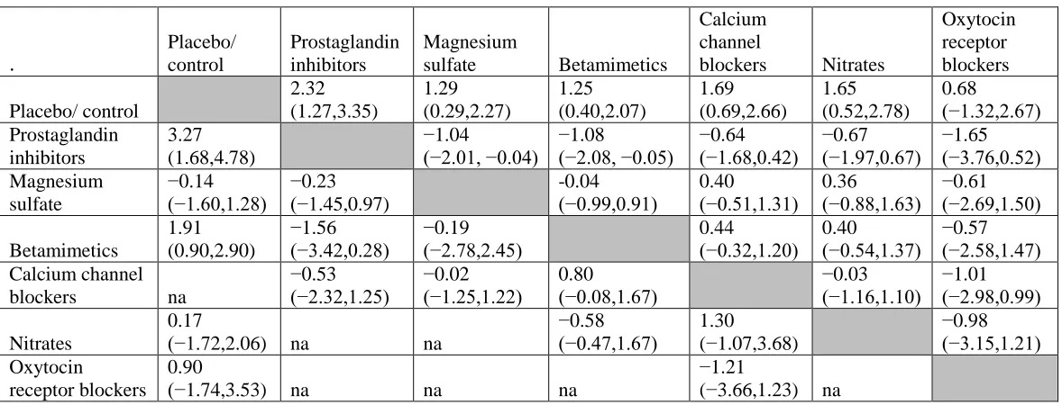
Table 2 reports the mean differences in EGA (in weeks) with their 95% CrIs. Colloquially
known as a ‘triangle table’, it displays findings from different analyses, in this case from the
direct, pairwise analyses and the NMA analysis. Values shown in the upper diagonal are the
MDs for the column header versus the row header and are derived from the NMA, and values
in the lower diagonal are the MDs for the row header versus the column header. This ensures
that the values are easily comparable across the two analyses. For example, the MD estimated
from the NMA (upper diagonal) for prostaglandin inhibitors vs placebo is 2.32 (95% CrI 1.27
to 3.35), suggesting that there is evidence that the intervention increases EGA at delivery, by
2.3 weeks, compared to placebo. In addition we can say that there is a 95% probability that
this increase is between 1.27 and 3.35 weeks. We can compare this to the MD estimated from
the direct evidence alone (lower diagonal) 3.27 (95% CrI 1.68 to 4.78). The first thing to note
is that the point estimates are close and the 95% CrIs overlap considerably. However, the
95% CrIs from the NMA are more precise. In contrast, the MD of Magnesium sulfate
compared to Placebo estimated from the direct evidence and the NMA appear contradictory,
with estimates in opposite direction, although the very wide 95%CrI for the pairwise
meta-analysis overlap with those obtained from the NMA, which are also narrower. The
consistency assumption was checked13 and some evidence of conflict between direct and
2.27), p-value=0.015). No explanation was found for this conflict but it was taken into
account when making decisions.
The empty cells in the lower diagonal denote that no direct evidence was available for that
comparison (for example, Calcium channel blockers vs Placebo), whereas the NMA can
make all the comparisons and show that there is evidence of an increase in EGA at delivery
for all interventions compared to Placebo, except Oxytocin receptor blockers (MD 0.68 95%
Table 2 Mean differences and 95% CrI for EGA at delivery (in weeks) from the pairwise and network meta-analyses. The upper diagonal displays the mean differences for the column intervention versus the row intervention, derived from the NMA. Values greater than 0 favour the column defining intervention. The lower diagonal displays the mean differences for the row intervention versus the column intervention, derived from direct comparisons only. Values greater than 0 favour the row defining the intervention. (Adapted from the NICE guideline13).
na: not available.
. Placebo/ control Prostaglandin inhibitors Magnesium
sulfate Betamimetics
Calcium channel
blockers Nitrates
Oxytocin receptor blockers Placebo/ control 2.32 (1.27,3.35) 1.29 (0.29,2.27) 1.25 (0.40,2.07) 1.69 (0.69,2.66) 1.65 (0.52,2.78) 0.68 (−1.32,2.67) Prostaglandin inhibitors 3.27 (1.68,4.78) −1.04
(−2.01, −0.04) −(−2.08, −0.05)1.08 −(−1.68,0.42)0.64 −(−1.97,0.67)0.67 −(−3.76,0.52)1.65
Magnesium sulfate
−0.14
(−1.60,1.28) −(−1.0.23 45,0.97)
-0.04
(−0.99,0.91) 0.40 (−0.51,1.31) 0.36 (−0.88,1.63) −(−2.69,1.50)0.61
Betamimetics
1.91 (0.90,2.90)
−1.56
(−3.42,0.28) −(−2.78,2.45)0.19
0.44
(−0.32,1.20) 0.40 (−0.54,1.37) −(−2.58,1.47)0.57
Calcium channel
blockers na
−0.53
(−2.32,1.25) −(−1.25,1.22)0.02 0.80 (−0.08,1.67)
−0.03
(−1.16,1.10) −(−2.98,0.99)1.01
Nitrates
0.17
(−1.72,2.06) na na
−0.58
(−0.47,1.67) 1.30 (−1.07,3.68)
−0.98
(−3.15,1.21)
Oxytocin
receptor blockers 0.90
(−1.74,3.53) na na na
−1.21
Triangle tables can also be used to report two different outcomes, with one in the top half and
the other in the bottom half. This can be a good way to display results from two important
outcomes, for example effectiveness and acceptability24 or other closely related outcomes,4
although it can be limited by the required width when there are many interventions. Similar
vertical displays can convey the same information14 15 and relative effects can also be
[image:13.595.73.492.354.497.2]presented as forest plots.13 14
Table 3 Posterior rank statistics and probabilities for the outcome EGA at delivery.
Rank statistics Probabilities
Interventions mean median 95%CrI best top 3
Placebo/control 6.74 7 (6,7) 0.00 0.00
Prostaglandin inhibitors 1.38 1 (1,4) 0.74 0.97
Magnesium sulphate 4.26 4 (2,6) 0.01 0.28
Betamimetics 4.48 5 (2,6) 0.00 0.16
Calcium channel blockers 2.84 3 (1,5) 0.07 0.76
Nitrates 3.04 3 (1,6) 0.13 0.65
Oxytocin receptor blockers 5.27 6 (1,7) 0.05 0.19
Table 3 shows treatment rankings and the probability that each intervention (or class) is the
‘best’ or in the top 3 for EGA at delivery. Here ranks are reported for effectiveness, such that
rank 1 means the intervention is most effective. Placebo has a mean rank of 6.74 and a
median rank of 7 (95% CrI 6 to 7). That is, on average, placebo was ranked approximately 7th
out of 7 treatments (i.e. worst) for gestational age at delivery. Conversely, prostaglandin
inhibitors were ranked 1st out of all 7 treatment classes and had a 74% probability of being
the most effective treatment and a 97% probability of being in the top three treatment classes
An alternative way of reporting ranks is to consider the cumulative probabilities using the
surface under the cumulative ranking curve (SUCRA)25 which transforms the cumulative
probabilities into a single value between 0 and 1, where a larger value indicates the more
effective treatment. This is often reported as a percentage.15
All probabilities, SUCRA values and rankings should be interpreted with caution as they are
very sensitive to the uncertainty in the relative treatment effects used to produce them.
Measures or displays which capture this uncertainty such as a table of rank statistics with
95% CrI (Table 3), rank probability plots (rankograms)10 14 25 or cumulative ranking
probability plots15 25 should be reported in preference to single values such as the probability
of being best or SUCRA. It is also imperative that ranking results are considered alongside
the estimates of relative treatment effects as a treatment could have a higher rank without
evidence of having a better effect than any of the others.
Importantly, all results should be interpreted taking into account the uncertainty in the
estimates (conveyed by the 95% CrI) as well as the risk of bias in the included evidence.
Tools that allow an examination of the impact of studies at risk of bias,26 27 and the impact of
changes in the evidence on the decision28 have been developed and can help to interpreting
the findings from a NMA.
CONCLUSIONS
When more than two interventions are being considered, synthesis of RCTs using an NMA
will ensure that all the relevant evidence, whether direct or indirect, is used to produce
coherent estimates of the relative effects of every intervention compared to every other. This
allows for more efficient use of the relevant evidence which can increase the precision of the
more robust than if only direct sources of evidence were included, that is they are less likely
to be influenced by the inclusion or exclusion of a single trial. The underlying assumption is
that there are no participant or study characteristics that would modify the relative treatment
effect of each treatment compared to every other.
Relying on multiple pairwise meta-analyses, each including a different set of trials may lead
to incoherent decisions and does not make the best use of the available evidence.
It is important to display NMA results carefully to aid interpretation and to clinically and
statistically assess the plausibility of the assumptions made.
COMPETING INTERESTS
None declared.
FUNDING
SD was funded by the Medical Research Council, UK (MR/M005232/1).
DC was supported by The Centre for the Development and Evaluation of Complex
Interventions for Public Health Improvement (DECIPHer), a UKCRC Public Health
Research Centre of Excellence. Joint funding (MR/KO232331/1) from the British Heart
Foundation, Cancer Research UK, Economic and Social Research Council, Medical Research
Council, the Welsh Government and the Wellcome Trust, under the auspices of the UK
REFERENCES
1. Cooper NJ, Sutton AJ, Ades AE, et al. Use of evidence in economic decision models: Practical issues and methodological challenges. Health Econ 2007;16(12):1277-86. doi: 10.1002/hec.1297
2. Efthimiou O, Mavridis D, Debray TPA, et al. Combining randomized and non-randomized evidence in network meta-analysis. Stat Med 2017;36(8):1210-26. doi:
10.1002/sim.7223
3. Corbett MS, Rice SJC, Madurasinghe V, et al. Acupuncture and other physical treatments for the relief of pain due to osteoarthritis of the knee: network meta-analysis.
Osteoarthritis Cartilage 2013;21:1290-98. doi: 10.1016/j.joca.2013.05.007
4. Mayo-Wilson E, Dias S, Mavranezouli I, et al. Psychological and pharmacological interventions for social anxiety disorder in adults: a systematic review and network meta-analysis. Lancet Psychiatry 2014;1:368-76. doi:
http://dx.doi.org/10.1016/S2215-0366(14)70329-3
5. Kriston L, von Wolff A, Westphal A, et al. Efficacy and acceptability of acutetreatments for persistent depressivedisorder: A network meta-analysis. Depression and Axiety 2014;31:621-30. doi: 10.1002/da.22236
6. Naci H, Dias S, Ades AE. Industry sponsorship bias in research findings: A network meta-analytic exploration of LDL cholesterol reduction in the randomised trials of statins BMJ 2014;349:g5741. doi: http://dx.doi.org/10.1136/bmj.g5741
7. Lu G, Ades A. Combination of direct and indirect evidence in mixed treatment comparisons. Stat Med 2004;23:3105-24.
8. Caldwell DM, Ades AE, Higgins JPT. Simultaneous comparison of multiple treatments: combining direct and indirect evidence. BMJ 2005;331:897-900. doi:
http://dx.doi.org/10.1136/bmj.331.7521.897
9. Dias S, Welton NJ, Sutton AJ, et al. Evidence Synthesis for Decision Making 1:
Introduction. Med Decis Making 2013;33:597-606. doi: 10.1177/0272989X13487604
10. Dias S, Ades AE, Welton NJ, et al. Network meta-analysis for decision making: Wiley 2018.
11. Bucher HC, Guyatt GH, Griffith LE, et al. The Results of Direct and Indirect Treatment Comparisons in Meta-Analysis of Randomized Controlled Trials. J Clin Epidemiol 1997;50(6):683-91.
12. Leucht S, Chaimani A, Cipriani AS, et al. Network meta-analyses should be the highest level of evidence in treatment guidelines. Eur Arch Psychiatry Clin Neurosci 2016;266(6):477-80. doi: 10.1007/s00406-016-0715-4
14. Haas DM, Caldwell DM, Kirkpatrick P, et al. Tocolytic therapy for preterm delivery: systematic review and network meta-analysis. Br Med J 2012;345 doi:
https://doi.org/10.1136/bmj.e6226
15. Zeng L, Tian J, Song F, et al. Corticosteroids for the prevention of bronchopulmonary dysplasia in preterm infants: a network meta-analysis. Arch Dis Child 2018;(in press)
16. Lu G, Ades A. Modeling between-trial variance structure in mixed treatment
comparisons. Biostatistics 2009;10(4):792-805. doi: 10.1093/biostatistics/kxp032 [published Online First: 2009/08/19]
17. Cooper NJ, Sutton AJ, Morris D, et al. Adressing between-study heterogeneity and inconsistency in mixed treatment comparisons: Application to stroke prevention treatments in individuals with non-rheumatic atrial fibrillation. Stat Med
2009;28:1861-81.
18. Spiegelhalter DJ. Incorporating Bayesian Ideas into Health-Care Evaluation. Statistical Science 2003;19:156-74.
19. Spiegelhalter DJ, Abrams KR, Myles J. Bayesian approaches to clinical trials and Health-Care Evaluation. New York: Wiley 2004.
20. Dias S, Welton NJ, Caldwell DM, et al. Checking Consistency in Mixed Treatment Comparison Meta-analysis. Stat Med 2010;29:932-44.
21. Cooper NJ, Kendrick D, Achana F, et al. Network Meta-analysis to Evaluate the Effectiveness of Interventions to Increase the Uptake of Smoke Alarms. Epidemiol Rev 2012;34:32-45. doi: 10.1093/epirev/mxr015
22. Dias S, Welton NJ, Sutton AJ, et al. Evidence Synthesis for Decision Making 4: Inconsistency in networks of evidence based on randomized controlled trials. Med Decis Making 2013;33:641-56. doi: 10.1177/0272989X12455847
23. Higgins JP, Jackson D, Barrett JK, et al. Consistency and inconsistency in network meta-analysis: concepts and models for multi-arm studies. Res Synth Methods
2012;3(2):98-110. doi: 10.1002/jrsm.1044
24. Cipriani A, Furukawa TA, Salanti G, et al. Comparative efficacy and acceptability of 12 new generation antidepressants: a multiple-treatments meta-analysis. Lancet
2009;373:746-58.
25. Salanti G, Ades AE, Ioannidis JPA. Graphical methods and numerical summaries for presenting results from multiple-treatment meta-analysis: an overview and tutorial. J Clin Epidemiol 2011;64:163-71.
26. Salanti G, Del Giovane C, Chaimani A, et al. Evaluating the Quality of Evidence from a Network Meta-Analysis. PLoS One 2014;9(7):e99682. doi:
10.1371/journal.pone.0099682