Article
1
Applications of Data Mining Algorithms for Network
2
Security
3
Kai Chain
4
Department of Computer and Information Science, Republic of China Military Academy, Kaohsiung 83059,
5
Taiwan; [email protected]
6
* Correspondence: [email protected]; Tel.: +886-7-743-8179; Fax: +886-7-747-9515
7
Abstract: Typical modern information systems are required to process copious data. Conventional
8
manual approaches can no longer effectively analyze such massive amounts of data, and thus
9
humans resort to smart techniques and tools to complement human effort. Currently, network
10
security events occur frequently, and generate abundant log and alert files. Processing such vast
11
quantities of data particularly requires smart techniques. This study reviewed several crucial
12
developments of existent data mining algorithms, including those that compile alerts generated by
13
heterogeneous IDSs into scenarios and employ various HMMs to detect complex network attacks.
14
Moreover, sequential pattern mining algorithms were examined to develop multi-step intrusion
15
detection. These studies can focus on applying these algorithms in practical settings to effectively
16
reduce the occurrence of false alerts. This article researched the application of data mining
17
algorithms in network security. The academic community has recently generated numerous
18
studies on this topic.
19
Keywords: data mining; network security; association rules; DDoS
20
21
1. Introduction
22
In short, data mining can be defined as the computational process of discovering meaningful
23
patterns or rules through the semi-automatic or automatic exploration and analysis of copious data.
24
The most commonly used analytical techniques for general data mining algorithms are cluster
25
analysis, classification analysis, link analysis, and sequence analysis. Cluster analysis is the task of
26
grouping data into multiple categories or clusters so that data within the same cluster share a higher
27
similarity with each other than with data in other clusters. Clustering can be used to identify dense
28
and sparse areas in the data space, thereby revealing the global distribution of the data and the
29
relationships between data characteristics. As the most widely applied data mining technique,
30
classification analysis can be used to model the relationships between crucial data or to predict data
31
trends. It involves classifying new data under predefined categories (e.g., normal and invaded). Two
32
of the most common classification methods are decision trees and rules. In 1993, Agrawal et al. at the
33
IBM Almaden Research Center proposed a problem concerning the association rules between
34
itemsets in a customer transaction database and presented the Apriori algorithm [13]. Their study
35
prompted intensive research on the problem of discovering association rules; this further facilitated
36
the application of data mining analysis techniques in various fields, particularly classification
37
analysis. Sequence analysis is a longitudinal analysis technique that identifies data characteristics by
38
employing temporal variables.
39
Cluster analysis, link analysis, and sequence analysis are the results of theories and research
40
that involved analysis of small-scale databases. Data mining has now extracted or integrated large
41
quantities of data from several large-scale databases. For instance, Wal-Mart utilizes an effective
42
data warehouse system that enables the provision of clear and detailed sales information to clients
43
and product suppliers; this enables presenting data regarding what products are most required by
44
its clients and when the clients need those products. Most importantly, Wal-Mart applied data
45
mining analyses of customer behavior models to increase the effectiveness of inventory control and
46
customer relationship management. The application of data mining for commercial purposes has
47
presently reached a certain level of maturity. In recent years, data mining techniques are often used
48
in research on security [1-12]. One of the most typical examples of a data mining application in
49
network security is an intrusion detection system (IDS). In general, an IDS collects a large quantity of
50
alert information. However, information security personnel cannot identify any associations from
51
large amounts of disorganized alert information. Nevertheless, an IDS that incorporates data mining
52
techniques facilitate identifying accurate and appropriate data characteristics from large quantities
53
of alert information by examining the association between multiple characteristics. The adequacy of
54
the data mining technique applied determines the usefulness of the data classification result, which
55
then affects the accuracy and effectiveness of intrusion detection. Thus, special attention must be
56
paid to the applicability of data mining algorithms under different scenarios; this explains why
57
further analysis should be performed on existing data mining algorithms.
58
[1-4] utilized an algorithm that augments existing scenarios with alerts generated by
59
heterogeneous IDSs; this algorithm considers each new alert by estimating the probability that this
60
new alert belongs to a given scenario and ascribes each alert to the most likely candidate scenario.
61
This involves real-time data mining on the basis of ideal scenarios. In addition, [1, 4] evaluated the
62
proposed algorithm by comparing it with two other probability estimation techniques; because this
63
method only requires simple data entry, it can serve as a more appropriate probability estimation
64
technique and is thereby more likely to obtain desired results. [5-9] employed hidden Markov
65
models (HMMs) to detect complex network attacks. Although a typical HMM is more effective in
66
detecting such complex intrusion events than are decision trees and neural networks, it has certain
67
drawbacks. Collaborative network attacks are often conducted over a long period (e.g., a few weeks
68
or months). Therefore, developing methods for detecting such slow-paced attacks in advance is one
69
of the primary research topics in this field. These methods must also be capable of detecting attacks
70
that involve highly complex methodologies, and must feature a set of procedures to detect
71
slow-paced attacks, and must be able to counteract attacks that have been detected. Sensor failures
72
or interference in transmission channels (such as open wireless networks), can affect the detection of
73
sequential attacks and cause errors. [10-12] proposed a sequential pattern mining technique that
74
incorporated alert information associated with distributed denial-of-service (DDoS) attacks and
75
reduce the repetition and complexity of abundant alert information received by the IDS, thereby
76
expediting the identification of the DDoS attack types. To identify the alert sequence of DDoS
77
attacks, [10] employed a particular HMM to compare algorithms. The comparison results indicated
78
that sequential pattern mining algorithms are more solid than other algorithms are because they do
79
not result in mutual exclusivity of correlation data during a DDoS attack and can increase the
80
accuracy of multi-step intrusion detection. The application of that HMM in experimental
81
comparison of algorithms verified whether the proposed algorithm exhibited favorable effects for
82
identifying the sequences of DDoS attacks and ensured effective reduction in alert complexity.
83
This paper is organized as follows. Section 2 elucidates the employed data mining algorithms.
84
Section 3 presents the data mining algorithms deemed as adequate for application to network
85
security. Section 4 presents the conclusions of this paper.
86
2. Data Mining Algorithms
87
In general, data mining involves converting collected data into preferred formats for analysis
88
and employing algorithms to derive useful intrusion detection models for identifying known or
89
unknown intrusion types. Data mining studies do not have a long history; they emerged mainly
90
from a study by Agrawal et al. (1993) [13], which stimulated widespread academic enthusiasm in
91
this topic.
92
Research manuscripts reporting large datasets that are deposited in a publicly available
93
database should specify where the data have been deposited and provide the relevant accession
94
numbers. If the accession numbers have not yet been obtained at the time of submission, please state
95
that they will be provided during review. They must be provided prior to publication.
Association rule mining is a procedure used to discover interesting associations or relevant
97
connections between itemsets in abundant data. As increasing amounts of data were collected and
98
stored, database users began to demonstrate interest in discovering association rules in their
99
databases. Discovery of interesting association rules is conductive to formulating commercial
100
policies, such as design categorization and cross selling. The purpose of such discovery (or mining)
101
is to identify any interesting relationships between items within a given data set. Support and
102
confidence are interestingness measures used for evaluating association rules; they reflect the
103
usefulness and certainty of association rules, respectively. Interestingness measures can also be used
104
to assess a model’s simplicity, certainty, utility, and novelty. Association rule mining is typically
105
performed with two steps:
106
(1) Find all frequent itemsets: Frequent itemsets are defined as itemsets with a high probability of
107
appearance in a database. If the obtained itemsets meet this definition, they are considered as
108
frequent itemsets.
109
(2) Generate strong association rules from qualified frequent itemsets: If the obtained itemsets meet
110
the criteria of minimum support and minimum confidence, they can be defined as strong
111
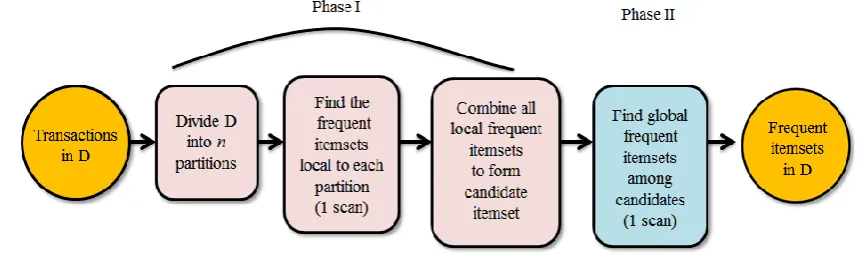
association rules.
112
The first step is clarified as follows. The Apriori algorithm is one of the most influential
113
algorithms used for association rule mining; it serves as the basis for comparing various algorithms
114
and is a basic technique for deriving different algorithms. This study designated the Apriori
115
algorithm was as the first algorithm to be thoroughly analyzed because it shares several key terms
116
with the other algorithms discussed herein. The Apriori algorithm requires verification on the basis
117
of the characteristics of frequent itemsets; to meet the criterion of this algorithm, all nonempty
118
subsets in a frequent itemset must be frequent. The Apriori algorithm involves layer-by-layer
119
iteration and mines (k+1)-itemsets by using k-itemsets. This mining process can be illustrated as
120
follows: First, find all frequent 1-itemsets and label them as L1. Subsequently, L1 is used to find
121
frequent 2-itemsets (L2), which are then used to find L3. This process is repeated until no more
122
frequent k-itemsets can be found. This algorithm scans the database when each search of Lk is
123
completed and generates candidate itemsets from the itemset L obtained in the previous search. The
124
candidate itemset meeting the Apriori criterion is then used as the itemset L for the following search.
125
To increase the efficiency of layer-by-layer iteration used for mining frequent itemsets, reducing
126
research space is a crucial goal of the Apriori algorithm. Figure 1 presents the pseudocode used in
127
the Apriori algorithm, where Input represents the transaction item of D, min_sup denotes the
128
minimum support count, and Output is the frequent itemset L in the database.
129
Once the first step has been completed by finding all frequent itemsets from the transaction
130
data in database D, the second step (generate strong association rules) can be performed
131
immediately. The identification of strong association rules requires meeting the criteria of minimum
132
support and minimum confidence. The following equation can be used to calculate confidence:
133
) ( _ ) ( _ ) ( ) ( A count suooprt B A count suooprt B A P B Aconfidence = =
(1)
134
where support_count(A∪B) denotes the number of transactions containing itemset A∪B and
135
support_count(A) denotes the number of transactions containing itemset A.
137
Figure 1. Apriori algorithm employed to discover frequent itemsets during Boolean association rule
138
mining
139
Because all rules are generated from frequent itemsets, each of these rules automatically satisfy
140
the minimum support count. Frequent itemsets and their support levels are included in the list of
141
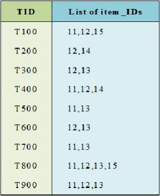
items to ensure they can be immediately mined. An example of applying the Apriori algorithm to
142
identify frequent itemsets in a database is presented as follows:
143
144
Figure 2. Data from the transaction database of Company Branch X
In this example, item IDs 11 and 12 are assumed to represent attacks in the field of network
146
security (they could just as easily be applied to represent other types of data, e.g., diapers and beer in
147
a supermarket). Frequent itemsets were generated from the following steps:
148
Step 1: In iteration 1, consider every item as a member of the candidate 1-itemset, C1. Scan all
149
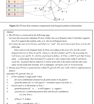
transactions roughly to count all items that appear (Figure 3).
150
151
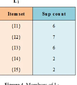
Figure 3. Members of C1
152
Step 2: Assume the minimum support count to be 2 (i.e., min_sup=2/9=22%) so that the frequent
153
1-itemset, L1, consists of candidate 1-itemsets meeting the threshold of the minimum support
154
count.
155
156
Figure 4. Members of L1
157
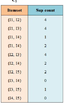
Step 3: Search for the frequent 2-itemset L2. Use the algorithm to generate the set of candidate
158
2-itemset,
C
26, where C2 consists of 21
L
C 2-itemsets (Figure 5).
159
Figure 5.Members of C2
161
Step 4: Scan the transactions in database D. Calculate the level of support of every candidate itemset
162
in C2 (Figure 6).
163
164
Figure 6. Support count of C2
165
Step 5: Confirm the frequent 2-itemset, L2, which consists of candidate 2-itemsets in C2 that satisfy
166
the criterion of greater than or equal to minimum support count.
167
168
Figure 7. Set L2
169
Step 6: First, let C2 = {{I1, I2, I3}, {I1, I2, I5}, {I1, I3, I5}, {I2, I3, I4}, {I2, I3, I5}, {I2, I4, I5}}. According to the
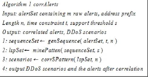
170
characteristics of the Apriori algorithm, all subsets in frequent itemsets should appear
171
frequently. Because any two items in the last four candidate itemsets do not appear in L2, these
172
are not frequent items, and thus these four candidate itemsets must be deleted from C3.
173
Therefore, their count must no longer be calculated when scanning D and confirming L3.
174
Notably, because the Apriori algorithm involves layer-by-layer iteration, once k itemsets are
175
given, the mining process starts by only checking whether their (k-1) subsets are frequent.
176
Step 7: Scan the transaction in database D to confirm whether L3 consists of candidate 3-itemsets in
177
C3 that satisfy the minimum support count (Figure 8).
179
Figure 8. Set C3
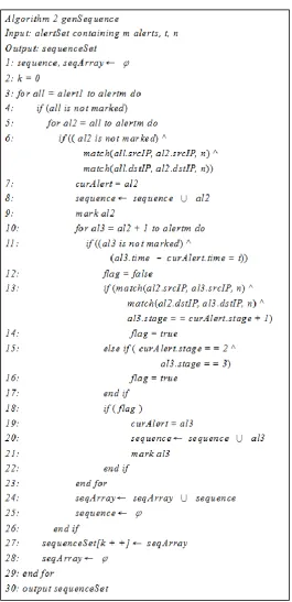
180
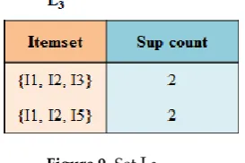
Step 8: Use the algorithm to generate the candidate 4-itemset, C4. Because subset {I2, I3, I5} did not
181
appear frequently in the {{I1, I2, I3, I5}} itemset, a result of C4, the subset was removed.
182
Accordingly, C4 was identified to be equal to an empty set, thereby terminating the algorithm
183
and identified all frequent itemsets in L3 (Figure 9).
184
185
Figure 9.Set L3
186
Now the example database is used to calculate which of the itemsets contain strong association
187
rules. The third data set derived from the example data, including frequent itemset l={I1, I2, I5},
188
indicates that the nonempty subsets of l are {I1, I2}, {I1, I5}, {I2, I5}, {I1}, {I2}, and {I5}. The resulting
189
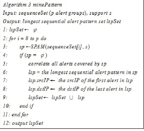
association rules are obtained from the aforementioned calculation method, each listed with its
190
confidence:
191
I1∧ I2⇒ I5,confidence = 2/4 = 50%
192
I1∧I5⇒ I2, confidence = 2/2 = 100%
193
I2∧I5⇒ I1, confidence = 2/2 = 100%
194
I1⇒I2∧ I5, confidence = 2/6 = 33%
195
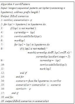
I2⇒I1∧ I5, confidence = 2/7 = 29%
196
I5⇒I1∧ I2, confidence = 2/2 = 100%
197
If the minimum confidence is 70%, then only the second, third, and sixth rules satisfy the threshold
198
of ≥70%. Thus, only these three items are strong association rules.
199
In [14, 17, 19], the main drawback of Apriori algorithm is that it must scan the database each
200
time when generating an association file. If the database contains abundant data, this method easily
201
increases the system load. To increase the efficiency of the Apriori algorithm, scholars have modified
202
this algorithm using specific methods. For instance, the hash-based technique can be used to
203
calculate the count of hash itemsets and reduce the size of the candidate k-itemset, Ck (k > 1). After
204
each transaction in the database is scanned, the frequent 1-itemset L1 is generated from the candidate
205
1-itemset in C1, and subsequently 2-itemsets can be generated from each transaction and then hashed
206
(i.e., mapped) into the buckets in the hash table, after which the corresponding bucket counts can be
207
increased (Figure 10). 2-itemsets with corresponding bucket counts in the hash table that are lower
208
than the support threshold are deemed as nonfrequent and are excluded from the candidate set. The
209
hash-based technique can largely reduce the number of k-itemsets examined (particularly when k =
210
2) [19].
212
Figure 10. Hash table, H2, for candidate 2-itemsets
213
Note: This table was generated by scanning the transactional database when determining L1 by C1. (If
214
the minimum support count is 3, then the itemsets in buckets 0, 1, 3, and 4 are nonfrequent and thus
215
should be removed from C2).
216
Transaction reduction can also be used to improve the Apriori algorithm. This method can
217
reduce the number of transactions scanned in future iterations. A transaction without any frequent
218
k-itemsets cannot contain any frequent (k+1)-itemsets. Thus, such transactions can be labeled or
219
removed; hence, subsequent database scans for j-itemsets (j > k) will no longer consider such
220
transactions. One variation of the Apriori algorithm involves partitioning the data to find candidate
221
itemsets. The partitioning technique requires only two database scans to mine frequent itemsets
222
(Figure 11). It consists of two phases. In phase I, the algorithm partitions the transactional data of D
223
into n nonoverlapping partitions. If the minimum support threshold in D is set as min_sup, then the
224
minimum support count for a partition should be min_sup × the number of transactions in the partition.
225
For each partition, all local frequent itemsets are found [17, 19].
226
227
Figure 11. Mining by the partitioning technique
228
Obtaining all local frequent k-itemsets requires only one database scan. All local frequent
229
itemsets can be treated as candidate itemsets for D. Therefore, collecting frequent itemsets from all
230
partitions enables generating the global candidate itemsets for D. In phase II, a second scan of D is
231
performed to evaluate the actual support count of each candidate to identify the global frequent
232
itemsets. This phase determines the partition size and the number of partitions so that each partition
233
can fit into main memory and thus be read only once in each phase [19].
234
Sampling can also be utilized to mine a subset of the given data. This technique involves
235
selecting a random sample S of the given database D and searching for frequent itemsets in S rather
236
than D. This method trades off certain degree of accuracy but increases efficiency. Because the
237
frequent itemsets are searched in S instead of D, some of the global frequent itemsets might be lost.
238
To reduce that possibility, a support threshold lower than the minimum support is adopted to
239
identify the frequent itemsets local to S (denoted LS). The rest of the database is then used to
240
calculate the actual frequencies of each itemset in LS to determine whether all the global frequent
241
itemsets are included in LS. If LS actually contains all the frequent itemsets in D, then only one scan of
242
D required. Otherwise, a second scan can be conducted to find any frequent itemsets that might have
243
been missed in the first scan. This sampling technique is particularly adequate when efficiency is
244
prioritized. Scholars have also proposed dynamic itemset counting as a method for enhancing the
Apriori algorithm. This approach adds candidate itemsets at various points during a scan and
246
partitions the database into blocks marked by start points. In contrast to standard Apriori, which
247
confirms new candidate itemsets only before each complete database scan, this variation can add
248
new candidate itemsets at any start point. This technique dynamically evaluates the support count of
249
all itemsets examined. If all subsets in an itemset are confirmed as frequent, then this itemset will be
250
considered as a new candidate itemset. Accordingly, this technique requires fewer scans than
251
standard Apriori does[14, 19].
252
Under various circumstances, the candidate itemsets generated by Apriori require an
253
examination method that will substantially reduce the size of the candidate itemsets, thereby
254
achieving favorable effectiveness of the Apriori algorithm. However, this algorithm must consider
255
the following two conditions:
256
(1) It may be required to produce a large number of candidate itemsets. For instance, if there are 104
257
frequent 1-itemsets, the Apriori algorithm will be required to generate more than 107 candidate
258
2-itemsets, during which the frequencies of all the candidate itemsets must be counted and
259
examined. In addition, to find frequent itemsets of length 100, such as {a1, …, a100}, a total of 2100
260
≈ 1030 candidate itemsets must be generated.
261
(2) It may be required to repeatedly scan the database and examine a large set of candidate itemsets
262
by pattern checking. Thus, a large amount of time is required to scan a database containing
263
abundant data.
264
[14-17] have improved previous algorithms by proposing an algorithm that mines the complete
265
set of frequent itemsets without requiring generation of candidate itemsets; the improved algorithm
266
involves using frequent pattern growth (FPG) and frequent pattern tree (FP-tree) methods. Because
267
this algorithm (hereinafter referred to as the FPG algorithm) possesses a higher efficiency than
268
conventional algorithms possess, the present study examined it further.
269
The FPG algorithm employs a divide-and-conquer strategy, illustrated as follows: First, it
270
compresses the database containing frequent itemsets into a FP-tree, which retains the itemset
271
association information. Subsequently, it partitions the compressed database into a set of conditional
272
databases, each of which is a special projected database that is associated with one frequent item.
273
Then it mines each database separately. The same example data were used to illustrate the algorithm
274
proposed by [14-17].
275
The first database scan of this algorithm is identical to that of the Apriori algorithm, which
276
derives the set of frequent items (1-itemsets) and their support (regarding count and frequency). Let
277
the minimum support count be 2. The set of frequent items is ranked in the order of descending
278
support count and the resulting set or list is denoted by L, thereby obtaining L=[I2:7, I1:6, I3:6, I4:2,
279
I5:2]. An FP-tree is subsequently constructed. The root of the tree is created and labeled with “null.”
280
Perform a second scan on database D. The items in each transaction are then arranged in L order
281
(i.e., ranked in the order of descending support count), with a branch created for each individual
282
transaction.
283
The scan of the first transaction, “T100:I1, I2, I5,” which contains three items (I2, I1, and I5,
284
sorted in L order), leads to the construction of the first branch of the tree with three nodes, (I2:1),
285
(I1:1), and (I5:1), where I2 is linked as a child to the root, I1 is linked to I2, and I5 is linked to I1. The
286
second transaction, “T200:I2, I4,” which contains the items I2 and I4 in L order, leads to a branch
287
where I2 is linked to the root and I4 is linked to I2. However, this branch shares a common prefix, I2,
288
with the existing path for T100. Therefore, the count of node I2 is increased by 1, and a new node,
289
(I4:1), is created; it is linked as a child to (I2:2). When adding a branch for a transaction, the count of
290
each node along a common prefix is generally increased by 1, and nodes for the items following the
291
prefix are created and linked accordingly.
292
To facilitate tree traversal, an item header table is constructed so that each item points to nodes
293
with the same ID in the tree through a chain of node-links. The tree obtained after scanning all the
294
transactions is shown in Figure 12, where all the associated node-links are illustrated. Therefore, the
295
problem of mining frequent patterns in databases is transformed into that of FP-tree mining.
297
Figure 12. FP-tree that contains compressed and frequent pattern information
298
299
Figure 13. Summary of the FPG algorithm, which mines frequent itemsets without generating
300
candidate itemsets
301
FP-tree mining is performed starting from each frequent length-1 pattern. Construct a
302
conditional pattern base (a sub-database that comprises the set of prefix paths in the FP-tree
303
co-occurring with the suffix pattern) for each pattern. Then, construct its conditional FP-tree, and
304
perform mining recursively on the tree. The pattern growth is attained by connecting the suffix
305
pattern with the frequent patterns generated from a conditional FP-tree.
306
Take I5 as an example. I5 occurs in two branches of the FP-tree displayed in Fig. 12. The paths
307
formed by these branches are (I2 I1 I5:1) and (I2 I1 I3 I5:1). Therefore, the two corresponding prefix
308
paths for I5 are (I2 I1:1) and (I2 I1 I3:1), which form its conditional pattern base. The I5-conditional
309
FP-tree contains only a single path, (I2:2 I1:2); I3 is included because its support count of 1 is less than
the minimum support count of 2. This single path generates all the combinations of frequent
311
patterns, which are (I2, I5: 2), (I1, I5: 2), and (I2, I1, I5: 2). The same process repeats when using other
312
items. The FPG algorithm is summarized in Figure 13.
313
In terms of mining long and short frequent patterns, the FPG algorithm exhibits higher
314
effectiveness, flexibility, and efficiency than the Apriori algorithm does.
315
3. Data Mining Algorithms Applicable in Network Security
316
Data related to network security require special attention in certain respects. For instance, they
317
may contain time packets so that the employed data mining algorithm may require adjustment
318
accordingly. Therefore, data mining algorithms applicable to network security were analyzed in the
319
present study to facilitate their subsequent application. Dain and Cunningham [1] proposed an
320
algorithm that organizes alerts generated by heterogeneous IDSs into scenarios; this algorithm
321
computes a new alert by estimating the probability that this new alert belongs to a given scenario
322
and adds alerts to the most likely candidate scenario. In a publication of the IEEE, Ourston et al. [5]
323
proposed a method that utilized HMMs to detect complex network attacks. The HMM is more
324
effective in detecting such complex intrusion events than are decision trees and neural networks.
325
This section uses [10, 18] to illustrate the application of data mining in network security. These
326
two studies proposed a sequential pattern mining technique that incorporated alert information
327
associated with DDoS attacks and reduced the repetition and complexity of abundant alert
328
information received by the IDS, thereby identifying the type of the DDoS attack. In addition, [10]
329
employed a particular HMM to compare algorithms. This method comprises four algorithms.
330
Algorithm 1 is the main mining loop and the other three algorithms are various extensions of
331
Algorithm 1.
332
In Algorithm 1, four variables are first inputted. The first variable is set as alertSet, which
333
denotes an alert set consisting of m raw alerts. The second to fourth variables are address prefix
334
length n, time constraint t, and support threshold s, respectively. The output variables are alerts that
335
have undergone correlation analysis and DDoS scenarios. Therefore, alertSet, address prefix length
336
n, and time constraint t are introduced as parameters into genSequence, a function that generates
337
sequential patterns. The output values produced from the calculation using genSequence are then
338
used as the parameters of genSequence and introduced into Algorithm 3, where sequenceSet and the
339
minimum support threshold s are inputted into function minePattern to identify the alert sample set
340
with the longest sequential pattern, labelled lspSet. Subsequently, lspSet and n are introduced into
341
the corrSPattern function to generate the desired DDoS scenarios. This entire process is completed
342
using input parameters and three functions (i.e., the following algorithms to be discussed).
343
344
Figure 14. Algorithm 1
345
The match (IP1, IP2, l) employed by the following algorithms is used as an example for
346
clarification. Let the addresses of IP1 and IP2 be 135.13.216.191 and 135.13.16.189, respectively. A
347
comparison of these addresses reveals that the third items of the two IP addresses are different.
348
Therefore, this indicates that n is the length of the first two identical IP addresses, namely n = 16.
350
Figure 15. Algorithm 2
351
Because real DDoS attacks at the final stage often contain packets generated from address
352
errors, adding alerts to a sequence facilitating counteracting this problem. The objective of
353
Algorithm 2 is to establish alert sequences by inputting variables m, t, and n to generate the desired
354
sequence. This algorithm consists of three loops. The first two loops define an alert group by
355
comparing IP addresses, namely comparing match (IP1, IP2, l) with the host address. Then, the third
356
loop extracts alerts during various attack stages from the previously obtained alert group to
357
construct alert sequences.
358
According to lines 6 and 7 of the following algorithm, all alerts that have been sorted are
359
marked, starting from alert 2. If an alert is not marked, its srcIP and dstIP will be compared with all
360
other srcIP and dstIP values. After the comparison, the original sequence and the alert will be
redefined into a new sequence, and this alert will be marked. For alerts that have already been
362
marked, alert time is used to determine whether they will be marked as false alerts, as suggested by
363
lines 11 and 12. If the result of subtracting an alert time from the current alert time is ≤ the inputted
364
variable t, then this alert is marked as a false alert. If the alert time meets the aforesaid criterion, then
365
whether the stage of this alert is higher than the current alert stage by one level will be checked, as
366
indicated by lines 13 and 14. If the alert stage is lower than the current stage, the alert is marked as a
367
false alert. The same rule applies to the rest of the alerts.
368
Algorithm 3 searches the sequential alert patterns from the alert groups created in algorithm 2.
369
Alerts found in each pattern are regarded as correlated. The longest sequential pattern is reserved in
370
the group because normal activities of a legitimate user may sometimes exhibit less frequent
371
patterns that are incorrectly captured into alert sequences. Such alerts are removed from further
372
analysis by this algorithm.
373
Algorithm 3 is as follows: Create a lspSet variable and set it as an empty set. Create a variable sp
374
and extract a portion of sequence to sp, as indicated in line 3. The sequence of sp is first used to find
375
long alert sequence (labelled lsp). Alert sequences meeting this lsp criterion are defined as srcIP and
376
dstIP. Finally, the identified lsp variable is added into the alert group, which is redefined as a new
377
group. The same process repeats until all lspSet sets found by the algorithm have been outputted.
378
379
Figure 16. Algorithm 3
380
Algorithm 4 generates DDoS scenarios mainly using the obtained sequential alert pattern
381
sample. The alert sample set with the longest sequential pattern is inputted into the algorithm and
382
loops of sequential patterns are used to generate a scenario catalog. In Algorithm 4, the first
383
lspatternn is required to end the alert at stage2 or stage3 particularly when producing correlation
384
data.
386
Figure 17. Algorithm 4
387
The test results confirmed that sequential pattern mining algorithms are more reliable than
388
other types of algorithm because they do not result in mutual exclusivity of correlation data during a
389
DDoS attack and can increase the accuracy of multi-step intrusion detection. Applying HMMs to
390
compare algorithms through comprehensive and experimental methods verifies whether the
391
proposed algorithm exhibits favorable effects for identifying the sequence of DDoS attacks and
392
ensures effective reduction in alert complexity.
393
We launched attacks with three tools, Nmap, Pizzaviat DDoS, Nikto, and compared them with
394
used algorithms and unused algorithms. Table 1 shows the number of times the alarm was detected.
395
The method of unused algorithms will repeatedly detect alerts, resulting in a much larger number
396
of times. The method of used algorithms will greatly reduce the number of alarms for the same
397
event.
398
Table 1. The Number of alerts
399
400
4. Conclusions
401
The importance of data mining in network security lies in its ability to automatically extract
402
hidden but crucial information from the alert and log data of large systems, thereby providing a
403
helpful tool for information security personnel to make decisions. Therefore, data mining has been
404
gradually introduced to network security studies that aim to investigate methods for detecting
unknown attacks before hazards occur and to minimize potential hazards caused by such attacks.
406
Section 3 indicates that sequential patterns can be used to generate a desired DDoS scenario. If the
407
effectiveness of the algorithm can be enhanced, a future version of the algorithm may be able to
408
construct multi-step attack scenarios; such an improvement will be beneficial to future practice.
409
Accordingly, a number of key algorithms related to this topic were analyzed in this study to
410
facilitate analyzing massive data in the future.
411
412
Author Contributions: Kai Chain conceived and designed the experiments; performed the experiments and
413
analyzed the data and wrote the paper.
414
415
Acknowledgments: This research was supported by MOST 106-2221-E-145-002.
416
Conflicts of Interest: The author declares no conflict of interest.
417
References
418
1. Dain OM and Cunningham RK. Fusing a heterogeneous alert stream into scenarios. In: Proceedings of the
419
2001 ACM Workshop on Data Mining for Security Applications, 14th September 2001; pp. 1-13.
420
2. Eckmann ST, Vigna G and Kemmerer RA. Statl: An attack language for statebased intrusion detection. J
421
Computer Security 2002; 10: 71-103.
422
3. Totel E, Vivinis B and Me L. A language driven IDS for event and alert correlation. In: SEC 2004; pp.
423
209-224.
424
4. Wang L, Ghorbani A and Li Y. Automatic multistep attack pattern discovering. Int J Network Security. 2010;
425
10: 142-152.
426
5. Ourston D, Matzner S, Stump W and Hopkins B. Applications of Hidden Markov Models to detecting
427
multi-stage network attacks. In: Proceedings of the 36th Ann. Hawaii International Conference on System
428
Science 2003; pp. 334.
429
6. Somayaji A and Forrest S. Automated response using system-call delays. In: Proceedings of the 9th
430
USENIX Security Symp, Denver, Colorado, 14 –17 August 2000; pp. 185-198.
431
7. Lee W, Stolfo SJ and Chan PK. Learning patterns from unix process execution traces for intrusion
432
detection. In: Proceedings of the AAAI97 workshop on AI Approaches to Fraud Detection and Risk
433
Management, AAAI Press, 1997; pp. 50-56.
434
8. Warrender C, Forrest S and Pearlmutter BA. Detecting intrusions using system calls: Alternative data
435
models. In: Proceedings of the IEEE Symp. on Security and Privacy, 1999; pp. 133-145.
436
9. Forrest S, Perelson AS, Allen L and Cherukuri R. Self-nonself discrimination in a computer. In: SP’94: Proc.
437
of the 1994 IEEE Computer Society, 1994; pp. 202.
438
10. Xiang G, Dong X and Yu G. Correlating Alerts with a Data Mining Based Approach. In: Proceedings of
439
the IEEE International Conference on e-Technoligy, e-Commerceande-Service, 29 March-1 April 2005.
440
11. AL-mamory SO and Zhang HL. A survey on IDS Alerts processing techniques. In: Proceedings of the 6th
441
WSEAS International Conference on Information Security and Privacy, Tenerife, Spain, 14-16 December
442
2007; pp. 69-78.
443
12. Cheng B, Liao G and Huang C. A novel probabilistic matching algorithm for multi stage attack forecasts.
444
IEEE J on Selected Areas in Comm. 2011; 29: 1438-1448.
445
13. Agrawal R, Imielinski T and Swami AN. Mining association rules between sets of items in large databases.
446
In: Proceedings of the 1993 ACM SIGMOD Intl. Conference on Management of Data, 1993; pp. 207-216.
447
14. Han J, Pei J and Yin Y. Mining frequent patterns without candidate generation. In: Proceedings of the
448
2000 ACM SIGMOD international conference on Management of data, 2000; pp. 1-12.
449
15. Leung CKS, Mateo MAF and Brajczuk DA. A tree-based approach for frequent pattern mining from
450
uncertain data. In: Proceedings of the Pacific-Asia Conference on Knowledge Discovery and Data Mining,
451
2008; pp. 653-661.
452
16. Zaki MJ, Li F and Yi K. Finding frequent items in probabilistic data. In: Proceedings of the 2008 ACM
453
SIGMOD international conference on Management of data, 2008; pp. 819-832.
454
17. Han J and Chang KCC. Data mining for web intelligence. Computer. 2002; 35: 64-70.
18. Stroeh K, Madeira ERM and Goldenstein SK. An approach to the correlation of security events based on
456
machine learning techniques. J Int Services and Applications. 2013; 4: 1-16.
457
19. Han J, Pei J and Kamber M. Data Mining Concepts and Techniques. 2011.