White Rose Research Online URL for this paper:
http://eprints.whiterose.ac.uk/119234/
Version: Accepted Version
Article:
Arnold, B., Goodwin, S.P., Griffiths, D.W. et al. (1 more author) (2017) How do binary
clusters form? Monthly Notices of the Royal Astronomical Society, 471 (2). pp. 2498-2507.
ISSN 0035-8711
https://doi.org/10.1093/mnras/stx1719
[email protected]
https://eprints.whiterose.ac.uk/
Reuse
Unless indicated otherwise, fulltext items are protected by copyright with all rights reserved. The copyright
exception in section 29 of the Copyright, Designs and Patents Act 1988 allows the making of a single copy
solely for the purpose of non-commercial research or private study within the limits of fair dealing. The
publisher or other rights-holder may allow further reproduction and re-use of this version - refer to the White
Rose Research Online record for this item. Where records identify the publisher as the copyright holder,
users can verify any specific terms of use on the publisher’s website.
Takedown
If you consider content in White Rose Research Online to be in breach of UK law, please notify us by
MNRAS000,1–10(2017) Preprint 12 July 2017 Compiled using MNRAS LATEX style file v3.0
How do binary clusters form?
Becky Arnold,
⋆
Simon P. Goodwin, D. W. Griffiths and Richard. J. Parker
†
Department of Physics and Astronomy, University of Sheffield, Sheffield S3 7RH, UK
Accepted XXX. Received YYY; in original form ZZZ
ABSTRACT
Approximately 10 per cent of star clusters are found in pairs, known as binary clusters. We propose a mechanism for binary cluster formation; we use N-body simu-lations to show that velocity substructure in a single (even fairly smooth) region can cause binary clusters to form. This process is highly stochastic and it is not obvious from a region’s initial conditions whether a binary will form and, if it does, which stars will end up in which cluster. We find the probability that a region will divide is mainly determined by its virial ratio, and a virial ratio above ‘equilibrium’ is generally necessary for binary formation. We also find that the mass ratio of the two clusters is strongly influenced by the initial degree of spatial substructure in the region.
Key words: stars: kinematics and dynamics – stars: formation – open clusters and
associations: general
1 INTRODUCTION
Star clusters are fascinating objects as they provide crucial tracers of the star formation, chemical, and dynamical his-tories of galaxies. Most star clusters are thought to form in a single star formation event and remain as coherent bound entities following this event. (If they disperse rapidly they are not ‘star clusters’ under this definition.)
An interesting observation is that star clusters are quite often found in pairs or higher-order systems (Rozhavskii et al. 1976). Such pairs are an expected result of chance line-ups (clusters far from each other appearing to be close due to viewing angle, (e.g. Conrad et al. 2017). However, once the effects of chance line-ups are accounted for a surplus of cluster pairs is still observed, indicating that at least some of them are related objects which are physically close to one another. Studies of the LMC and SMC appear to show that roughly 10 per cent of clusters are in such pairs, which are known as binary clusters (Pietrzynski & Udalski 2000). The fraction of binary clusters in the MW has been found to be lower than this by some studies (Subramaniam et al. 1995), and about the same by others (De La Fuente Marcos & de La Fuente Marcos 2009).
Binary clusters are systematically younger than single clusters e.g. half of the clusters in binaries identified byDe La Fuente Marcos & de La Fuente Marcos(2009) are<25
Myr old, and almost all of those are in coeval pairs (see also Dieball et al. 2002;Palma et al. 2016). This is not an unusual
⋆ E-mail: [email protected]
† Royal Society Dorothy Hodgkin Fellow
result; the clusters that constitute a binary are often coeval (e.g.Kontizas et al. 1993;Mucciarelli et al. 2012). The most obvious explanation for pairs of clusters with very similar ages is that their formation was linked in some way, but the origins of these pairs are not understood.
Some multiplicity may be expected as a natural conse-quence of structure in molecular clouds (e.g.Elmegreen & Falgarone 1996). This paper presents an additional mech-anism for binary cluster formation: the division of a single star forming region (as seen to some degree in e.g.Goodwin & Whitworth 2004andParker et al. 2014).
In this paper we present a series ofN-body simulations. We show that, at least for some initial conditions, binary clusters are a fairly common outcome of the dynamical evo-lution of these systems. We describe our initial conditions in Section 2, present detailed results from a small set of sim-ulations in Section 3, conduct a parameter space study in Section 4, and and conclude in Section 5.
2 METHOD
We perform purely N-body simulations of fractal distribu-tions using the kira integrator, which is part of starlab
(Portegies Zwart et al. 1999; Portegies Zwart et al. 2001). Our simulations include no gas, no stellar evolution, and no external tidal fields. As such, they are very simple nu-merical experiments, but we argue that they capture all of the essential physics of a possible binary cluster formation mechanism. We run the simulations for 20 Myr.
©2017 The Authors
2.1 Positions and masses
Artificial young star forming regions are constructed using the box fractal method, which is described in detail in Good-win & Whitworth(2004). In brief, box fractals are generated by creating a cube and placing a ‘parent’ star at its centre. The cube is divided into subcubes, which have ‘child’ stars placed at their centres, with noise added to avoid a gridlike structure. Parent stars are deleted, and the children become the new generation of parents. This process is repeated un-til the desired number of stars, N, has been overproduced. Finally, a sphere of radiusRis cut from the initial box, and stars are randomly deleted until the N stars remain. We take regions withN=1000andR=2pc as our ‘standard’.
The degree of substructure (space-filling) is set by the frac-tal dimensionD(e.g. 1.6 is very substructured, 3 is roughly uniform density).
The stars are assigned masses drawn randomly from the Maschberger IMF (Maschberger 2013) with the scale param-eter µ=0.2 M⊙, and the high mass exponent αI MF =2.3.
The low mass exponent is calculated using β = 1.4. The
lower and upper mass limits used are 0.1 and 50 M⊙. The
Maschberger IMF is similar to the Chabrier IMF (Chabrier 2003) and the Kroupa IMF (Kroupa 2002).
2.2 Velocity structure
As will become apparent later in the results, the velocity structure of the fractal is very important. The gas from which stars form is known to have complex (turbulent) struc-ture (Larson 1981), and the stars in young regions appear to retain this structure (e.g.F˝ur´esz et al. 2006;Jeffries et al. 2014;Tobin et al. 2015;Wright et al. 2016).
To mimic this we assign stars velocities such that the regions are velocity coherent; stars that form near each other have initially similar velocities. We do this by one of two methods: either inheriting velocities from their parent as the fractal is generated (this is the main method used), or by imposing velocities from a divergence-free turbulent velocity field.
Inherited velocities: Following Goodwin & Whit-worth(2004), parent stars at the first level are given a ran-dom velocity. Child stars inheret their parent’s velocity plus a random component which scales with the depth in the frac-tal (i.e. the random component is large at the higher-levels, and becomes smaller). This creates a velocity field in which stars that are close together in space tend to have initially similar velocities.
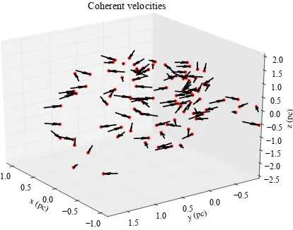
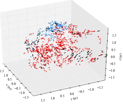
Fig. 1 shows an N = 100 fractal produced by this
method. Star positions are indicated by red dots plotted in three dimensional space, and their velocities by arrows. As can be seen, the velocity field has local ‘coherence’. For example, the stars on the upper far-left of the figure are all moving to the right, while on the lower far-left there is a group of four stars moving downwards and slightly to the left.
Turbulent velocity fields: We generate divergence-free turbulent velocity fields with a power spectrum P(k) =k−αfor the region, whereα= 2 (e.g.Burkert & Bo-denheimer 2000;Lomax et al. 2014). The initial positions of the stars are mapped onto these fields, and they are assigned the field velocity at their location.
x (pc ) −1.0 −0.5 0.0 0.5 1.0
y (pc)
[image:3.595.335.542.109.272.2]−0.5 0.0 0.5 1.0 1.5 z (pc ) −2.5 −2.0 −1.5 −1.0 −0.5 0.0 0.5 1.0 1.5 2.0 Coherent velocities
[image:3.595.305.544.456.521.2]Figure 1.A set of initial conditions demonstrating velocity struc-ture in a region with 100 stars and a radius of 1 pc. The red dots indicate the positions of stars, and their velocity vectors are de-noted by black arrows.
Table 1.Letters are used to describe the initial conditions in each set of simulations. Two parameters are varied: the fractal dimensionD, and the virial ratio (i.e. the ratio of kinetic to po-tential energy)αvir. Highly-substructured simulations (D=1.6)
are denoted by the letter ‘H’, moderate substructure (D=2.2) is
denoted by the letter ‘M’, and smooth structure (D=2.9) by ‘S’.
Simulations of cool regions (αvir =0.3) are denoted by ‘C’,
viri-alised regions (αvir =0.5) are denoted by ‘V’, and warm regions
(αvir=0.7) by ‘W’.
D
1.6 2.2 2.9
αvir
0.3 HC MC SC
0.5 HV MV SV
0.7 HW MW SW
2.3 Virial ratio
Finally, the velocities are scaled to set the desired virial ratio,
αvir=T /|Ω|(whereT is the total kinetic energy, andΩthe total potential energy).
2.4 Ensembles
We perform simulations with fractal dimensions ofD=1.6,
2.2 and 2.9. When D = 1.6 we describe the
simula-tions as highly-substructured (‘H’),D=2.2is
moderately-substructured (‘M’), and smooth (‘S’) whenD =2.9. The
velocities are scaled to have a virial ratio ofαvir=0.3(cool, ‘C’),0.5(virialised, ‘V’), or 0.7 (warm, ‘W’).
We refer to the initial conditions of a simulation by these identifying letters, e.g. ‘MW’ is a moderately-substructured, warm region (D=2.2,αvir=0.7). A summary of the
simu-lations is shown in Table 1.
How do binary clusters form?
3
2.5 Cluster finding
In Appendix A we describe our cluster finding algorithm. This is used to distinguish bound ‘clusters’ within our larger regions as they evolve. It is able to determine which stars are locally bound to a particular object, and which are ‘halo’ stars. The algorithm is not perfect, and sometimes struggles when applied to regions with ambiguous or unusual mor-phologies. However it allows us to avoid ‘by-eye’ determina-tions of membership when the region evolves to a distinct single or binary cluster, which occurs in the vast majority of cases.
3 THE FORMATION OF A BINARY CLUSTER
First we will examine the process of binary cluster formation in a small set of simulations. This allows us to investigate the process in detail. Twelve MW simulations (D = 2.2,
αvir = 0.7) are chosen at random for this; binary cluster formation is fairly common in the MW ensemble, and the number 12 is chosen to produce an easily readable figure. Later we will examine parameter space to see which initial conditions are most likely to form binary clusters.
3.1 An ensemble of moderately-substructured, warm regions
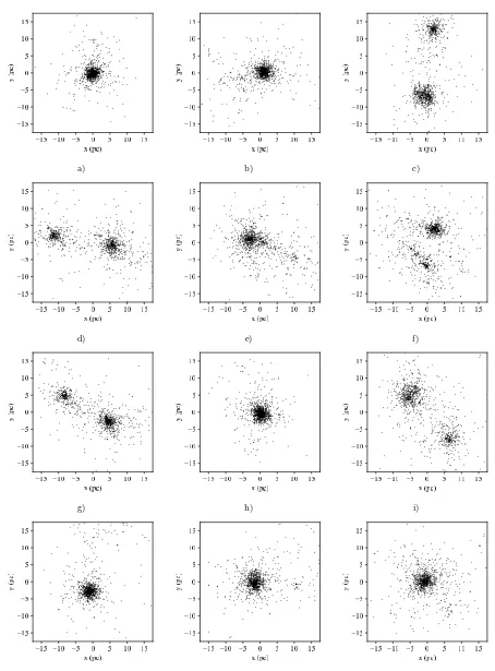
In Fig. 2 we show the stellar distributions of each of the 12 regions after 20 Myr. The distributions are presented inx-y projection in 35 pc-by-35 pc boxes. These simulations all use inherited velocities (see Section 2.2).
A visual inspection of Fig. 2 shows that distinct binary clusters form in 4 of the 12 realisations, in subfigures (c), (d), (g), and (i)1
.
Simulation (f) has an overdensity at roughly (2 pc, -7 pc) which could be a small companion cluster. Despite the other structure in the region and the significant halo, our cluster-finding algorithm does distinguish it as a distinct entity. We therefore define simulation (f) as a binary cluster. Simulations (a), (b), (h), (j), (k) and (l) have evolved into single, central star clusters.
Simulation (e) has also evolved into a single cluster, but is elongated. Elongated clusters are discussed more later, in Section 4.3.
It is important to remember that all 12 simulations had statistically the same initial conditions, only the random number seed has been changed. The wide range of morpholo-gies apparent at the end of the simulations is not particularly surprising, as the evolution of substructured initial condi-tions is known to be highly stochastic (Parker & Goodwin 2012;Allison et al. 2010).
1
Interestingly, in (c), (d) and (g) there are ‘bridges’ of stars link-ing the two clusters. These ‘bridges’ are present when viewed in 3D suggesting they are real features. Similar bridges have been found in observations of binary clusters (Dieball & Grebel 1998;
Dieball & Grebel 2000;Minniti et al. 2004).
3.2 Future evolution
We may na¨ıvely expect binary clusters to orbit one another in the same manner binary stars do, however in these simu-lations the two clusters move directly apart, and are usually unbound from each-other. At the end of the simulations two of the binaries are unbound, two arejustunbound, and one is bound. The bound binary could recombine at some point in the future, in fact such recombanations are observed in the full ensemble of simulations, and are discussed in Section 4. In reality such mergers may be less likely as the Galactic potential could shear the clusters away from each other.
Typically the relative velocities of the clusters in our simulations are only∼1km s-1, so they could remain
obser-vationally associated for many 10s of Myr even if they are formally unbound.
3.3 The division of a star forming region
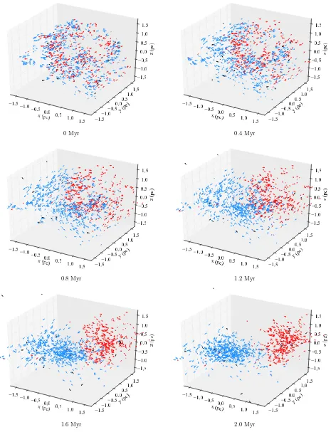
We now examine how binary clusters form in more detail. In Fig. 3 we show the evolution of the region from panel (c) of Fig. 2 for the first 2 Myr of its evolution in steps of 0.4 Myr (in panel (c) of Fig. 2 the region is 20 Myr old). We identify the two clusters at 3 Myr when they are distinct, well-separated entities with our cluster finding algorithm. Then, at each time we colour code the stars bywhich cluster they will eventually be members of, blue for the cluster on the left, red for the cluster on the right, and black for unbound to either cluster. Therefore, all of the red stars in the top left panel at 0 Myr are the same stars as are coloured red in the final panel (and all panels inbetween). For each star we also plot its velocity vector (an arrow pointing from the position of the star).
It is immediately obvious from inspection of Fig. 3 that the stars from each cluster are initially very well-mixed. The red and blue stars (that will end-up in the right- and left-hand clusters respectively) are each found everywhere in the region at 0 Myr. Without the colour coding (which is based on where we know they will be in the future), from the positions of the stars alone it would be (a) impossible to tell that this region would evolve into a binary cluster, and (b) impossible to tell which stars would end-up in which cluster. This is true forallthe simulations in this paper.
As the region evolves the stars which will end-up in each cluster begin to separate out into two distinct sub-clusters. At 0.4 Myr there has been some separation; while the three classes of stars are still generally mixed, clumps of just red or blue stars have begun to form. After 0.8 Myr there has been further separation, and these clumps appear to have grown. By 1.2 Myr the blue stars are predominantly on the left, and the red stars are predominantly on the right. At 1.6 Myr the two groups of stars have formed roughly spherical shapes, but it isn’t until 2 Myr that clusters are well separated.
This behaviour appears to be the result of the initial velocity coherence. Inspection of Fig. 3 shows that whilst the red and blue points are initially mixed, they are not completely randomly distributed. Even at the very begin-ning there are small groups of either red or blue stars with low velocity dispersion. These groups go on to merge with other groups with (usually) similar velocities. The details of the velocity structure in this particular case mean that a significant number of stars move in roughly the same two
a) b) c)
d) e) f)
g) h) i)
[image:5.595.65.519.95.710.2]j) k) l)
How do binary clusters form?
5
directions. In cases where the velocity structure is such that they tend to move in many different directions then a single cluster is formed.
We run 50 simulations with the same input parameters as the previus set, i.e. moderately-substructured and warm, but the velocities are randomised. As one would expect all 50 of the regions evolve into single clusters. This confirms that velocity structure is necessary for a binary cluster to form.
Given the importance of velocity structure to the for-mation of binary clusters, it is reasonable to wonder to what extent this might be an artifact of the (somewhat unphysi-cal) generation of velocity coherence via inheritance. To test this we re-run the 12 simulations with coherence set up using a different method: velocities are sampled from a turbulent velocity field (see Section 2.2). The initial spatial distribu-tions of the simuladistribu-tions are unchanged.
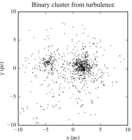
Binary clusters form in two of these simulations (ex-ample shown in Fig. 4). In Fig. 5 we show the initial condi-tions of the realisation that evolves into the binary cluster in Fig. 4: the blue stars are those that end-up in the left-hand cluster, the red stars end-up in the right-hand cluster, and black stars are unbound to either cluster (cf. Fig. 3).
There is arguably less mixing in Fig. 5 than in the first panel of Fig. 3; the blue points are mostly initially close to-gether towards the upper-centre. However, without colour coding it is still not obvious that this part of the initial con-ditions will produce a separate cluster. So, as was the case in the simulations with inherited velocities, we argue that from the initial conditions (a) it is not at all obvious whether a binary cluster will be produced, and (b) it is impossible to say which stars will end up in which cluster (or be unbound). To review, binary clusters form in 2/12 simulations which use a turbulent velocity field, compared to 5/12 bi-nary clusters from inherited velocities. This test consists of too few simulations to estimate the different rates of binary formation using each of the methods, and a detailed investi-gation of different methods of setting-up velocity coherence is beyond the scope of this paper. The important points here are
1. Velocity coherence is necessary for binary clusters to form. 2. Two independent methods are used to generate coherence and binary formation results from both. Therefore our re-sults are not an artifact of the method used to initialise velocity structure.
4 PARAMETER SPACE STUDY
In this section we explore parameter space to probe which initial conditions can form binary clusters, and investigate the properties of the binary clusters which form.
As described in Section 2, nine ensembles of 50 sim-ulations are performed. The fractal dimension D is varied such that D = 1.6, 2.2, or 2.9 (highly-substructured (H),
moderately-substructured (M), and smmoth (S)). The virial factorαviris varied such thatαvir=0.3, 0.5 or 0.7 (cool (C), virialised (V), or warm (W)). The simulations are run for 20 Myr, and are summarised in Table 1.
4.1 Which initial conditions produce binary clusters?
We classify the final state of each simulation as one of three basic categories.
Binary clusters:two clearly distinguished clusters as iden-tified by the cluster finder and/or by eye. (In highly ambigu-ous cases when the cluster finder struggles preference is given to the by-eye conclusion). Note that 4 of our 450 simulations develop triple clusters. For the sake of simplicity we classify these as binary clusters.
Single clusters:one significant cluster (often with an un-bound ‘halo’ of stars).
Binary merger:a region that is a single cluster at 20 Myr, but was a binary cluster at some earlier time. This may be because a binary cluster formed and then merged into a sin-gle cluster, or one of the two clusters dissolved. Therefore, depending on the time of an observation, they could be seen by an observer as a (young) binary or a single cluster2
The classifications of of the HV and HW simulations should be treated with some caution as their long-lived sub-structure makes several of them difficult to classify. Four of the 450 simulations in this parameter space study are deemed ‘unclassifiable’, and are omitted.
In Fig. 6 we present the fractions of regions which evolve into single, binary-merger and binary clusters. These frac-tions approximate the probability of each outcome, and the multinomial distribution is used to calculated to one sigma confidence where the true probability lies, which is indicated in Fig. 6 by error bars.
The top panel of Fig. 6 shows the results for the highly-substructured (D=1.6) ensembles with virial ratios
αvir=0.3, 0.5, and 0.7 on thex-axis. The green circles are the fractions of single clusters, yellow diamonds are the fraction of binary mergers, and red diamonds the fraction of binary clusters. The middle panel of Fig. 6 is the same plot but for the moderately-substructured (D=2.2) ensembles, and the
bottom panel is for smooth (D=2.9) ensembles.
Each panel of Fig. 6 shows the same essential behaviour: binary clusters are more common as the virial ratio in-creases.
When the regions are dynamically cool (αvir=0.3, the left-most results in each panel), almost all the simulations form a single cluster. This is as expected, as a dynamically cool distribution will collapse and erase substructure ( Alli-son et al. 2009;Parker et al. 2014). However, the cool ensem-bles also produce some binary mergers; even though these regions are collapsing, velocity structure can allow them to ‘divide’ for some amount of time.
When regions have moderate virial ratio (αvir=0.5, the middle results in each panel) the fraction of regions which evolve into single clusters drops, and the fraction that evolve into binary mergers increases concurrently. The exception to this is the H simulations, where both binaries and binary mergers form.
When the regions are dynamically warm (αvir=0.7, the right-most results in each panel), the fraction of single
clus-2
The longest observed interlude between division and recombi-nation of a binary merger in these simulations is∼20Myr. At the
other extreme, some binary mergers separate so briefly they are only ‘binary clusters’ for∼1Myr.
0 Myr 0.4 Myr
0.8 Myr 1.2 Myr
[image:7.595.71.536.112.719.2]1.6 Myr 2.0 Myr
How do binary clusters form?
7
−10 −5 0 5 10
x (pc) −10
−5 0 5 10
y (pc
)
[image:8.595.51.277.104.343.2]Binary cluster from turbulence
Figure 4.A 20 pc-by-20 pcx-yprojection of a simulation with initially turbulent velocities after 20 Myr. The region has devel-oped into a binary cluster.
ters drops again and the fraction of binary mergers drops somewhat at all levels of substructure. In contrast, the frac-tion of binary clusters increases
The main result from ensembles of different initial con-ditions as summarised in Fig. 6 are:
1) Higherαvirincreases the probability that a region will di-vide
2) Binary clusters mainly form in dynamically warm regions.
4.2 ‘Micro-clusters’
Regions do not always divide into a clean binary or sin-gle clusters. In particular, the highly-substructured regions (D=1.6), especially with high virial ratio (αvir=0.5, 0.7), can often form several small, bound objects we refer to as ‘micro-clusters’. Fig. 7 shows an example of an HW simu-lation at 20 Myr with four micro-clusters (indicated by the red arrows).
Whilst these micro-clusters are able to survive 20 Myr, they will have short lifetimes because they only contains tens of members so their two-body relaxation time is very short. Nevertheless, they could be observed around young clusters and mistaken for independent objects instead of potential evidence that the region was initially highly substructured.
4.3 Elongated clusters
Some S regions undergo a period of elongation followed by collapse within the first∼5 Myr. This is observed mainly in S simulations, and is most common when αvir is high. An
example is shown in Fig. 8
4.4 Cluster mass ratios
We determine the mass ratios of the binary clusters, (and binary-mergers when they are distinct entities) using the cluster finding algorithm. In highly ambiguous cases, where the algorithm struggles, the cluster memberships are de-termined by eye. This means that in some cases a partic-ularmass ratio should be treated with caution. However the trends we describe should not be affected by a small number of ambiguities. Note that we define mass ratios as the mass of the lighter cluster divided by the mass of the heavier one. Therefore if the cluster masses are very different the mass ratio is low, and if their masses are fairly equal the mass ratio is high, with a maximum of unity.
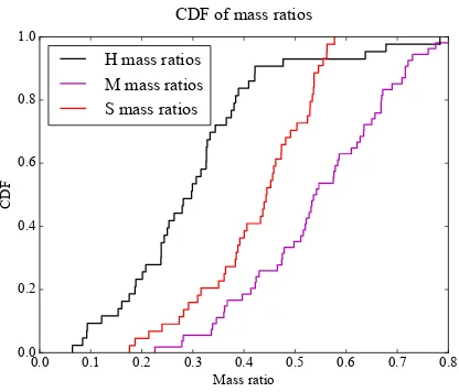
The cumulative distribution functions (CDFs) of highly-substructred (H, black line), moderately-substructed (M, purple line) and smooth (S, red line) binary mass ratios are shown in Fig. 9. Most binary clusters are from warm sim-ulations (αvir=0.7) as these are the ensembles that produce the vast majority of binary clusters.
From Fig. 9 it is clear that the mass ratio distributions for each level of substructure are distinct (a KS test gives a P-value<10−4for any pair of distributions, confirming that
they are statistically different).
Binary clusters that form from highly-substructred ini-tial conditions (H, black line) tend to have low mass ratios (i.e very unequal cluster masses) almost all being 0.1–0.4 (median 0.3).
Binary clusters that form from smooth initial conditions (S, red line) have higher mass ratios, almost all between 0.3– 0.6 (median 0.44).
Binary clusters that form from moderately-substructred initial conditions (M, purple line) have generally higher mass ratios still, ranging mostly from 0.4–0.8 (median 0.54).
We may have expected to see a sequence in mass ra-tio distribura-tions that moves from highly-substructred, to moderately-substructred, to smooth. Instead the smooth re-gion’s mass ratios are intermediate between those of the highly and moderately-substrucured regions.
We explain this by first considering the smooth regions (red line) as a baseline. They have no spatial structure, so their mass ratios are entirely due to velocity structure.
The moderately-substructured regions contain fairly large spatial structures, which themselves are correlated with the velocity structure. As a result there are often nat-ural ‘starting points’ for sizable portions of the regions to separate from the rest, resulting in more even mass ratios.
In contrast, the highly-substructured regions contain many small spatial structures which may divide from the main cluster, resulting in many low mass ratio systems.
4.5 Comparison with observations
Probably the best-known binary clusters, h andχPer, have a mass ratio of 0.76 (masses of 3700 and 2800M⊙respectively,
Slesnick et al. 2002), which, from Fig. 9, suggests moderate initial substructure. However this is only a single binary clus-ter, which may not be representative of the conditons that the majority binary clusters form from.
A catalogue of well measured mass ratios could poten-tially provide observational clues as to the initial conditions of the regions that produce real-world binary clusters.
x (pc
)
−1.5
−1.0
−0.5
0.0
0.5
1.0
1.5
y (pc)
−1.5
−1.0
−0.5
0.0
0.5
1.0
1.5
z (pc
)
−1.5
−1.0
−0.5
0.0
[image:9.595.116.543.131.490.2]0.5
1.0
1.5
Turbulent initial conditions
Figure 5.The initial conditions of the simulation shown in Fig. 4, which evolves into a binary cluster. Inspection of the figure clearly shows velocity coherence, which is produced by mapping the positions of the stars onto a turbulent velocity field. The colour coding is the same as described in Fig. 3.
fortunately, the current state of observational data cannot provide good constraints (Conrad et al. 2017). However, if more than one mechanism is responsible for binary cluster formation, the cluster mass ratio distribution would be a combination of those produced by all the different mecha-nisms, and would be much harder to interpret.
5 CONCLUSIONS
We perform ensembles ofN-body simulations ofN =1000,
R =2pc regions, which are evolved for 20 Myr. These
re-gions start with fractal dimensions of D = 1.6, 2.0 or 2.9
(from highly-substructured to smooth), and virial ratios (the ratio of kinetic to potential energies) ofαvir=0.3, 0.5 or 0.7 (from cool to warm). The velocities of stars are ‘coherent’; stars that are initially close together tend to have similar velocities.
We find that single star forming regions can dynamically evolve into binary clusters, (although this is not necessarily the only way binary clusters may form). We find that initial
velocity structure is necessary for a region to divide, and in all cases it is essentially impossible to determine from the initial state of a region:
1. If a binary cluster will form (although most of the re-gions thatdo form binaries are initially dynamically warm (αvir=0.7)).
2. Which stars will end up in which component of the binary cluster.
The two clusters move directly apart from one another with relative velocities typically∼1km s−1, so pairs will
ap-pear associated for 10s Myr. In some cases the clusters re-main bound to one another, and recombine at a later time. We describe these as binary-mergers, and they are most com-mon in regions that begin in virial equilibrium.
How do binary clusters form?
9
0.3 0.5 0.7
Virial ratio αvir 0.0 0.2 0.4 0.6 0.8 1.0 P roba bi li ty
Outcomes of H simulations
Single Merger Binary F ra ct ion
0.3 0.5 0.7
Virial ratio αvir 0.0 0.2 0.4 0.6 0.8 1.0 P roba bi li ty
Outcomes of M simulations
Single Merger Binary F ra ct ion
0.3 0.5 0.7
Virial ratio αvir 0.0 0.2 0.4 0.6 0.8 1.0 P roba bi li ty
Outcomes of S simulations
[image:10.595.49.258.86.655.2]Single Merger Binary F ra ct ion
Figure 6. The fraction of regions which evolve into single, binary-merger and binary clusters for each set of simulations. The highly-substructured (H) simulation results are shown in the top panel, the moderately-substructured (M) simulations in the mid-dle panel, and the smooth (S) simulations in the bottom panel. The x axis separates the simulations by their virial ratioαvir(0.3,
0.5 or 0.7). The fraction of regions in a given set of simulations which evolve into single clusters is indicated by green circles. The fraction of binary-mergers is indicated by wide yellow diamonds, and the fraction of binary clusters is shown by narrow red dia-monds. x (pc) −20 −10 0 10 20 y (pc ) −20 −10 0 10 20 z (pc ) −20 −10 0 10 20 Microclusters
Figure 7.A highly-substructured, dynamically warm region that has been evolved for 20 Myr. The star’s positions are indicated by dots in a 40 pc-by-40 pc-by-40 pc box. The simulation has developed numerous long lived overdensities. We call these over-densities ‘microclusters’, and they are highlighted by red arrows.
x (pc)0 −2 −4 2
4
y (pc)
[image:10.595.311.540.97.281.2]−4 −2 0 2 4 z (pc ) −4 −2 0 2 4 Elongated cluster
Figure 8.An initially smooth, virialised region after evolving for 3 Myr. It has developed an elongated shape which collapses back into a sphere within the next few Myr.
ACKNOWLEDGEMENTS
BA acknowledges PhD funding from the University of Sheffield, and DWG from the STFC. RJP acknowledges support from the Royal Society in the form of a Dorothy Hodgkin Fellowship. Thanks also to Søren Larsen for useful discussions.
REFERENCES
Allison R. J., Goodwin S. P., Parker R. J., de Grijs R., Portegies Zwart S. F., Kouwenhoven M. B. N., 2009,ApJ,700, L99
Allison R. J., Goodwin S. P., Parker R. J., Portegies Zwart S. F., de Grijs R., 2010,MNRAS,407, 1098
Burkert A., Bodenheimer P., 2000,ApJ,543, 822
Chabrier G., 2003,PASP,115, 763
[image:10.595.334.545.379.537.2]0.0 0.1 0.2 0.3 0.4 0.5 0.6 0.7 0.8 Mass ratio
0.0 0.2 0.4 0.6 0.8 1.0
CD
F
CDF of mass ratios
[image:11.595.54.262.102.280.2]H mass ratios M mass ratios S mass ratios
Figure 9.Cumulative distribution functions of the cluster mass ratios. The CDF for highly-substructured (H) simulations is plot-ted by a black line, the moderately-substructured (M) simulations by a magenta line and the smooth (S) simulations by a red line.
Conrad C., et al., 2017,A&A,600, A106
De La Fuente Marcos R., de La Fuente Marcos C., 2009,A&A,
500, L13
Dieball A., Grebel E. K., 1998, A&A,339, 773
Dieball A., Grebel E. K., 2000, A&A,358, 897
Dieball A., M¨uller H., Grebel E. K., 2002,A&A,391, 547
Elmegreen B. G., Falgarone E., 1996,ApJ,471, 816
F˝ur´esz G., et al., 2006,ApJ,648, 1090
Goodwin S. P., Whitworth A. P., 2004,A&A,413, 929
Jeffries R. D., et al., 2014,A&A,563, A94
Kontizas E., Kontizas M., Michalitsianos A., 1993, A&A,267, 59
Kroupa P., 2002,Science,295, 82
Larson R. B., 1981,MNRAS,194, 809
Lomax O., Whitworth A. P., Hubber D. A., Stamatellos D., Walch S., 2014,MNRAS,439, 3039
Maschberger T., 2013,MNRAS,429, 1725
Minniti D., Rejkuba M., Funes J. G., Kennicutt Jr. R. C., 2004,
ApJ,612, 215
Mucciarelli A., Origlia L., Ferraro F. R., Bellazzini M., Lanzoni B., 2012,ApJ,746, L19
Palma T., Gramajo L. V., Clari´a J. J., Lares M., Geisler D., Ahumada A. V., 2016,A&A,586, A41
Parker R. J., Goodwin S. P., 2012,MNRAS,424, 272
Parker R. J., Wright N. J., Goodwin S. P., Meyer M. R., 2014,
MNRAS,438, 620
Pietrzynski G., Udalski A., 2000, Acta Astron.,50, 355
Portegies Zwart S. F., Makino J., McMillan S. L. W., Hut P., 1999, A&A,348, 117
Portegies Zwart S. F., McMillan S. L. W., Hut P., Makino J., 2001,MNRAS,321, 199
Rozhavskii F. G., Kuz’mina V. A., Vasilevskii A. E., 1976, Astro-physics,12, 204
Slesnick C. L., Hillenbrand L. A., Massey P., 2002,ApJ,576, 880
Subramaniam A., Gorti U., Sagar R., Bhatt H. C., 1995, A&A,
302, 86
Tobin J. J., Hartmann L., F˝ur´esz G., Hsu W.-H., Mateo M., 2015,
AJ,149, 119
Wright N. J., Bouy H., Drew J. E., Sarro L. M., Bertin E., Cuil-landre J.-C., Barrado D., 2016,MNRAS,460, 2593
APPENDIX A: THE CLUSTER-FINDING ALGORITHM
We briefly describe how clusters are identified in a snapshot of the simulation.
• Step 1: Distinguish areas of high stellar density. Space is divided into equally sized boxes by a three dimen-sional grid. The resolution of this grid is initially low, and it is increased until 75 per cent of the stars of the stars are contained within at least 20 boxes. This resolution distin-guishes areas of high stellar density without being too fine or coarse.
• Step 2: Find the position of a cluster.
The box containing the most stars is located. By defini-tion, clusters are regions with many stars so this box will be at, or close to, the centre of a cluster. The centre of mass and centre of velocity of the stars in this box is calculated. The mass of stars in this box is used to crudely estimate the mass of the cluster.
• Step 3: Identify cluster members.
The program goes through each star and calculates its kinetic and potential energy relative to the position, velocity, and mass determined in step 2. Bound stars are identified as cluster members.
• Step 4: Identify further cluster members.
The centre of mass, centre of velocity, and total mass of the cluster members is calculated. Step 3 is repeated using these values, i.e. the kinetic and potential energy of each star relative to this position, velocity, and mass is calculated to identify further members.
• Step 5: Find additional clusters.
Steps 2-5 repeat. In order to prevent the same cluster being identified multiple times, stars that have already been identified as members of a cluster are excluded in step 2. Therefore when all the clusters have been identified the box containing the most stars, as identified by step 2, contains so few stars it could not reasonably be the centre of a new cluster. The program stops searching for additional clusters after that point. Any remaining stars are determined to be unbound.
• Step 6: Clean up.
This step prevents the order in which the clusters are iden-tified from influencing the final membership lists. All infor-mation on which stars belong to which cluster is thrown away; only the positions, masses, and velocities of the clus-ters are retained. The potential and kinetic energy of each star compared to these clusters is calculated to determine which cluster (if any) the star is most strongly bound to. This produces the final membership list for each cluster. The mass, centre of mass, and centre of velocity of each cluster is recalculated using this membership list.