Bayesian Analysis for Photolithographic Models

Rochester Institute of Technology

RIT Scholar Works

Theses Thesis/Dissertation Collections

6-19-2017

Bayesian Analysis for Photolithographic Models

Andrew M. Burbine

Follow this and additional works at:https://scholarworks.rit.edu/theses

This Thesis is brought to you for free and open access by the Thesis/Dissertation Collections at RIT Scholar Works. It has been accepted for inclusion in Theses by an authorized administrator of RIT Scholar Works. For more information, please contactritscholarworks@rit.edu.

Recommended Citation

1

Bayesian Analysis for Photolithographic Models

By

Andrew M. Burbine

A Thesis Submitted

in Partial Fulfillment

of the Requirements for the Degree of

Master of Science

in

Microelectronic Engineering

Approved by:

Prof. _____________________________ Dr. Bruce W. Smith (Thesis Advisor)

Prof. _____________________________

Dr. Robert Pearson (Committee Member & Program Director)

Prof. _____________________________ Dr. Dale Ewbank (Committee Member)

Prof. _____________________________ Dr. Ernest Fokoue (Committee Member)

Dr. John L. Sturtevant (External Collaborator)

Rochester Institute of Technology Kate Gleason College of Engineering

2

Abstract

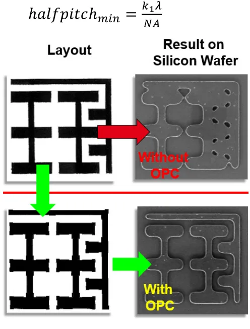
The use of optical proximity correction (OPC) as a resolution enhancement technique

(RET) in microelectronic photolithographic manufacturing demands increasingly accurate

models of the systems in use. Model building and inference techniques in the data science

community have seen great strides in the past two decades in the field of Bayesian statistics.

This work aims to demonstrate the predictive power of using Bayesian analysis as a method for

parameter selection in lithographic models by probabilistically considering the uncertainty in

physical model parameters and the wafer data used to calibrate them. We will consider the error

between simulated and measured critical dimensions (CDs) as Student’s t-distributed random variables which will inform our likelihood function, via sums of log-probabilities, to maximize

Bayes’ rule and generate posterior distributions for each parameter. Through the use of a

Markov chain Monte Carlo (MCMC) algorithm, the model’s parameter space is explored to

find the most credible parameter values. We use an affine invariant ensemble sampler (AIES)

which instantiates many walkers which semi-independently explore the space in parallel, which lets us exploit the slow model evaluation time. Posterior predictive checks are used to analyze

the quality of the models that use parameter values from their highest density intervals (HDIs).

Finally, we explore the concept of model hierarchy, which is a flexible method of adding

3

Table of Contents

Abstract ... 2

List of Figures ... 5

Introduction and Motivation ... 10

Chapter 1 – Photolithographic Systems ... 13

Chapter 2 – Statistical Modeling ... 19

Probability Distributions ... 19

Uncertainties as Distributions ... 22

Linear Regression... 26

Chapter 3 – Bayesian Analysis ... 30

Bayes’ Theorem ... 30

Markov chain Monte Carlo algorithms ... 31

The Linear Model example, revisited ... 33

The Likelihood Function ... 35

Implementation in Python ... 37

Chapter 4 – Results and Analysis... 41

Initial, exploratory run ... 41

Adding n & k of the resist and ARC ... 46

Hierarchy in the Model ... 50

4

Posterior predictive checking and comparison to incumbent process ... 58

Conclusions ... 60

5

List of Figures

Figure 1: An example of using optical proximity correction to increase the image fidelity during

pattern transfer ... 11

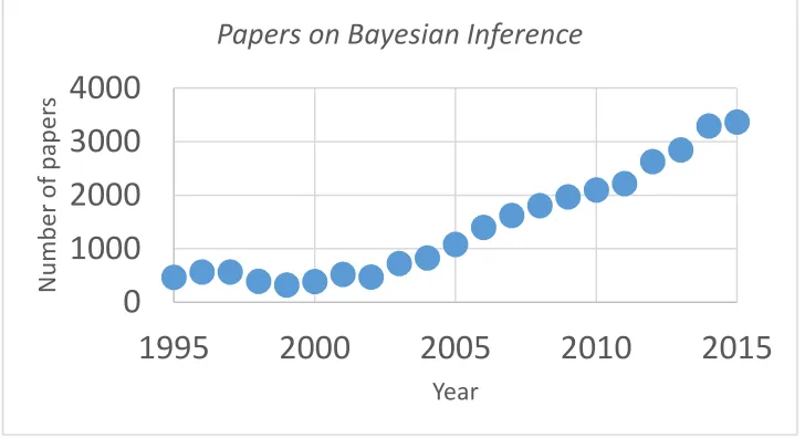
Figure 2: There's been a large increase on published papers on Bayesian inference and analysis

methods. ... 13

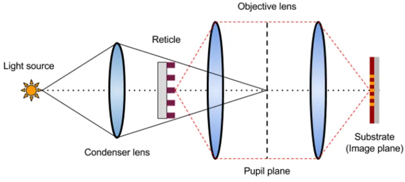
Figure 3: Schematic of a Köhler illumination system used for photolithographic processing.

The pattern on the mask is minified by 4x and transferred to the wafer, where its latent image

indicates where the deprotection reactions in the photoresist will result in removal during

development ... 14

Figure 4: Various illustrations of image fidelity as k1 and the minimum feature size decrease

for a 193nm non-immersion system at 0.85 NA. At k1 = 0.3, the feature no longer resolves a

usable resist contour. However, through various techniques described in the figure, imaging is

still possible. [7] ... 16

Figure 5: Screenshot from Calibre WORKbench showing the simulated contour (red) of a

photomask (white) and a gauge (vertical line) which measures the CD at this location. . 17

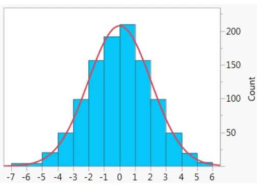
Figure 6: Histogram of 1000 points generated from a normal distribution with mean 0 and

standard deviation 2. In red is the exact probability density function for the distribution.21

Figure 7: Illustration from Sir Francis Galton of "the bean machine" which physically

demonstrates the central limit theorem. ... 21

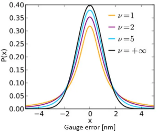
Figure 8: Student's t-distribution with various values for ν_{, showing the change in the tails of}

the distribution. As ν _{approaches infinity, the Student’s t-distribution becomes the normal}

6

Figure 9: Sample 2D data generated with error bars representing measurement uncertainty. The

line represents the function used to generate the sample points. This data will be used in

subsequent examples of linear modeling; mtrue = -0.9594, btrue = 4.294 and ftrue = 0.534 (where

f * y * U(0, 1))... 27

Figure 10: Sample data and the model generated by least squares regression. Parameter

estimates are mls = -1.104 ± 0.016 and bls = 5.441 ± 0.091 ... 28

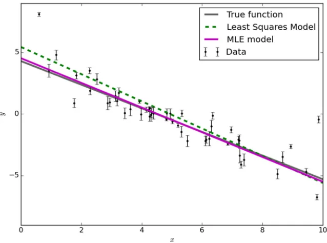
Figure 11: Sample data with the maximum likelihood model solution, in magenta. Parameter

estimates are mmle = -1.003, bmle = 4.528 and fmle = 0.454. ... 29

Figure 12: Figure with caption from Goodman and Weare's publication showing a stretch move

[17] ... 32

Figure 13: Posterior distribution for the parameters in the linear model. Top plots are 1D

histograms, others are bivariate density plots. True values are shown in blue lines... 34

Figure 14: Red shows the true model. The rest of the lines are samples form the posterior

distribution showing various candidate models. Bayesian analysis sees the solutions as a

probabalistic entity. ... 34

Figure 15: Flow diagram describing the goal of Bayesian analysis for photolithographic

modeling. The model, which has fixed and free parameters, describe the photolithographic

manufacturing process and produce simulated contours of the resist based on the mask layout.

These are ideally as close as possible to the CD measurements from the wafer fab, which are

shown to be drawn from a distribution due to stochastic effects. ... 37

Figure 16: Flow diagram for generating the posterior distribution ... 39

Figure 17: The seven dimensional posterior distribution using 100 gauges during the posterior

7

Figure 18: 2nd calibration from an independent random sample of 100 gauges from the master

set. ... 44

Figure 19: 3rd calibration from an independent random sample of 100 gauges from the master

set ... 45

Figure 20: The full 11 dimensional posterior space. Blue lines indicate values given with the

testcase for each parameter. Thus, differences between the given and posterior indicate the

benefit from optimizing these parameters. ... 47

Figure 21: Magnified plot of the resist and ARC n & k posteriors ... 49

Figure 22: Graphical representation of the simple one level model hierarchy used so far.50

Figure 23: Graphical representation of two level model hierarchy using feature types to group

the gauges. ... 51

Figure 24: The posterior distribution triangle plot for the two-level hierarchical model and n &

k film stack parameters. ... 52

Figure 25: The posterior distribution triangle plot for the simple two-level hierarchical model.

... 53

Figure 26: Priors (red), likelihoods (blue) and posteriors (violet) for various samples of identical

true and unknown distribution with a uniform prior. [24] ... 54

Figure 27: Priors (red), likelihoods (blue) and posteriors (violet) for various samples of identical

true and unknown distribution with a normal prior close to the likelihood. [24] ... 55

Figure 28: Priors (red), likelihoods (blue) and posteriors (violet) for various samples of identical

true and unknown distribution with a prior far from the likelihood. [24] ... 56

Figure 29: Posterior distributions for two optimziations on just mask parameters comparing the

9

List of Tables

Table 1: Parameters in the model along with their associated prior distributions and absolute

limits. Beamfocus and metrology plane are relative to the top of the resist stack, such that 0 =

top, and positive is into the plane of the wafer. ... 38

Table 2: The film stack properties added to the parameter space along with their priors and

truncated limits ... 46

Table 3: Comparison of nm RMS error between simulated models and wafer data for basic and

complex models generated with different random samples of gauges. Compare to incumbent

10

Introduction and Motivation

The pace of microelectronics manufacturing capability is dictated each year by the

International Technology Roadmap for Semiconductors (ITRS) [1] with goals centered on

scaling devices smaller and smaller and addressing associated challenges, such as mitigating

line edge roughness and increasing critical dimension (CD) uniformity across a wafer.

Historically, these challenges rested on the shoulders of lithographers and the chemists who

created the photoresists necessary for patterning. Today, the challenges are also felt by the

layout designers, who must seek regularity in their designs and plan for such things as multiple

patterning, and the tool manufacturers who must integrate increased metrology and uniformity

controls on intra- and inter-wafer effects.

The goal of solving these challenges is to increase the processing power and memory

capabilities for the ever expanding usage of electronics, which enable new technologies and a

higher quality of life. Amusingly, one of the key uses for increased processing power and

memory capabilities is in the lithographic field itself – the modern lithographer operates at the

limits of his or her lithographic scanning tool and must make use of many resolution

enhancement techniques (RET), chief among them, optical proximity correction (OPC), an

example of which can be seen in Figure 1. Accurate OPC models require powerful computers

to operate on a full-chip layout due to the immense number of patterns [2].

OPC compensates for image errors due to operating at or near the diffraction-limited

resolutions of the scanners used to transfer the design intent image to the wafer. A measure of

a system’s resolution is typically given by Rayleigh’s criterion, seen in Equation 1, where the

smallest critical feature width, or minimum half pitch, is determined by the wavelength λ_{, the}

11

ℎℎ

=

(1)

Figure 1: An example of using optical proximity correction to increase the image fidelity during pattern transfer

Thus, for a modern 193 nm immersion system, operating at an NA of 1.35 and a k1

factor of 0.3, a minimum half pitch of about 42 nm is achievable. OPC is a key method for

reducing the usable k1 factor of a manufacturing process, decreasing the minimum pitch and

keeping pace with the ITRS roadmap.

In order to apply OPC to a full-chip layout, fast models are needed to simulate resist

contours from layout geometries. Model-based OPC methods simulate the changes to the layout

and seek to find solutions to make dense patterns resolve with robustness to small changes in

dose and focus (the so called process window). These models make use of physically based

parameters from the system, such as film stack properties like the n and k of various materials in models of the photomask which effect the transmission and phase of the light used for

anti-12

reflective coatings, under-layers and the substrate itself), the wavelength of light used in

exposure and a jones pupil of the optics of the scanner and any pellicle (protective film over the

photomask) [4].

These parameters are tuned in a model training exercise by matching simulated CD

measurements to measurements taken from a wafer. Thousands of CDs are collected by a CD

scanning electron microscope (CDSEM) which produce images similar to the right side of

Figure 1. Current day practice involves minimizing the root mean square error of the measured

CDs to the simulated CDs via gradient-descent like optimization methods.

Unfortunately, this ignores a key aspect of the model building process: uncertainty.

Measurements taken from a CDSEM are not always accurate due to the low resolution of the

SEM and the difficulty in resolving the edge of a sloped photoresist sidewall profile from a

top-down image. Additionally, there are uncertainties in some of the parameters which are fixed in

the models, such as the thickness of the photoresist or its optical constants (refractive index n and extinction coefficient k). Though in the past these uncertainties may have been well beyond the scope of critical sources of error in the modeling process, today’s OPC demands accuracy

to the single digit nanometer or below level.

Additionally, modelers may often have reasons to believe parameters are more likely to

have accurate solutions at certain values over others. For example, the mask absorber sidewall

angle is often expected to be at 86 degrees, plus or minus a degree, rather than at, for example, 90 degrees. Modelers may also have expectations on the amount of variance possible for a

parameter, for example the photoresist thickness might vary by 1-2 nm but not more.

Under a Bayesian framework these uncertainties and a priori knowledge can be

13

from a distribution of possible values. Additionally, CDSEM measurements are often taken

from several dies or wafers and have the number of images used to produce the single average

value reported, as well as the standard deviation of those measurements. This information can

be directly incorporated into the cost function that drives the optimization procedure.

The goal of this work is to apply Bayesian analytic methods to produce

photolithographic models that better utilize available information and incorporate the

uncertainties that exist in both the model parameters and the measurements that are used to

inform those parameters. Bayesian methods have seen an increase in usage (Figure 2) and

maturity as increased computational power has enabled stronger algorithms needed to converge

to solutions for high-dimensional parameter spaces.

Figure 2: There's been a large increase on published papers on Bayesian inference and analysis methods.

Chapter 1 – Photolithographic Systems

Photolithography is the process by which a pattern is transferred from a mask, or reticle,

to a wafer using light and a photosensitive thin film (photoresist). After the wafer is exposed to

DUV (or EUV) light, in a positive-tone resist, those areas can be dissolved away with a

developer solution, typically a strong base. This then enables either etching into the material

0

1000

2000

3000

4000

1995

2000

2005

2010

2015

N u m b e r o f p a p e rs Year

14

below the photoresist or deposition of a new material in the resulting voids. Thus, lithography

is at the center of constructing microelectronic devices: repeated deposition and etching steps

are done in specific patterns created by a series of exposures for different layers of the device.

These layers form and provide connections between transistors, which are arranged to create

logic gates that are used for computation, memory storage or other functions.

Figure 3: Schematic of a Köhler illumination system used for photolithographic processing. The pattern on the mask is minified by 4x and transferred to the wafer, where its latent image indicates where the deprotection reactions in the

photoresist will result in removal during development

Since smaller and smaller feature sizes enable more computing power per area of a chip,

we must consider what defines an optical system’s capability. Equation 1 defines the minimum

halfpitch by what is known as Rayleigh’s criterion. From this equation two things are

immediately apparent: increasing the lens size, NA, and reducing the wavelength, λ_{, will reduce}

the feature size. For several decades, these were the main strategies for continued scaling in the

industry, which moved swiftly from 365 nm to 248 nm and finally (for transmissive optics) 193

nm. Tools are currently in evaluation and technology research and development at 13.5 nm

(EUV, reflective optics) after almost a decade since 193i was introduced for use in production

15

through the use of water between the lens and substrate [5]. Research was done exploring 157

nm as a successor to 193 nm, but ultimately did not occur due to a myriad of challenges [6].

The other parameter in the equation, k1, is known as a ‘process factor’ which

encapsulates many other performance criterion in the system, such as photoresist resolution (the

ability of the photoresist to threshold the image with minimal loss), mask properties (such as a

thin absorber to limit 3D mask effects) and illumination properties (see below). k1 can be seen

as a compromise between image degradation and the photoresist’s robust ability to capture

low-intensity modulation to form binary images.

Figure 4 illustrates how k1 for a non-immersion (0.85 NA) 193 nm system relates to

image fidelity and various so-called resolution enhancement techniques (RET) used to undo its

effect on imaging. When k1 is high, imaging is easily achieved by the system and as it decreases

with the minimum desired feature size, eventually the image fidelity drops below a tenable

level. Off-axis imaging (OAI) refers to the use of partially incoherent sources. Initial OAI

technologies employed various primitives, such as dipoles and quasars, to improve imaging.

Today, sources can be pixelized and are produced through source-mask optimization (SMO) as

16

Figure 4: Various illustrations of image fidelity as k1 and the minimum feature size decrease for a 193nm non-immersion

system at 0.85 NA. At k1 = 0.3, the feature no longer resolves a usable resist contour. However, through various techniques

described in the figure, imaging is still possible. [7]

Finally, a key technology for enabling low-k1 imaging and increasing the resolution of

photolithographic systems is optical proximity correction (OPC), shown in the figure as the

ultimate solution for producing usable images for a given process condition. Figure 5 shows the

simulation output using a photolithographic model in Calibre WORKbench. During iterations

of OPC, edges of feature polygons are moved with the goal of minimizing the edge placement

17

Figure 5: Screenshot from Calibre WORKbench showing the simulated contour (red) of a photomask (white) and a gauge (vertical line) which measures the CD at this location.

Early OPC techniques were rule-based – edges were moved based on a rule deck to do

such things as compensate line-end pullback by adding hammerhead shapes to tip-to-tip

features or biasing the edge of an array with smaller features to compensate for edge effects.

Rule-based techniques were fast and could be performed on an entire chip to improve imaging

performance. However, eventually, special algorithms were developed to be able to perform

simulations of aerial images fast enough to be usable on a full chip [8], [9], [10]. Additionally,

computing power advanced enough to enable such simulations, which is to say that advancing

lithographic techniques enabled the ability to further advance lithographic techniques.

Thus, model-based OPC was born and a new branch of enabling technologies and

methodologies came along with it. These methods include: sum of coherent systems

decomposition (SOCS), domain decomposition methods (DDM), hybrid Hopkins-Abbe

method for source sectorization (HHA) and resist compact models (CM1) [11], [12], [13],

[14]. Each enabled more accurate simulation of the final resist or etch contour on the wafer

level from simulations of the photomask through the imaging system. Typically, models are

calibrated to wafer CD measurements on a test mask, which contains large arrays of various

18

perform OPC, these models are used to modify the full chip geometries to match the design

intent (or target layer) within some tolerances, usually through focus to mitigate errors caused

by wafer topography.

The subject of this thesis is to improve the accuracy of the models used by finding

more accurate representations of the physical parameters in the model. To do this, we

consider the parameters as coming from unknown distributions and the CDs collected of the

wafer as having uncertainty derived from being drawn from a distribution, based on the

standard deviation of those measurements. These distributions are represented in a Bayesian

19

Chapter 2 – Statistical Modeling

Probability Distributions

In the field of data science, models are created to describe data sets which can be used to make

predictions, gain insight on the system that produced the data set, or characterize the stochastic

elements of the system. Statistical modeling differs from mathematical modeling in that part or

parts of the model are non-deterministic; some variables in the model do not have specific

values but instead are drawn from probability distributions.

A probability distribution is a mathematical definition of a function that satisfies several

properties: 1) evaluates to a non-negative number for all real inputs, 2) the sum (or integral) for

all possible inputs is 1, and 3) the probability of a specific value (or a value between bounds) is

the result of the evaluation of the function.

The simplest and most classic example of a probability distribution is the Bernoulli

distribution, which describes a system in which the outcome is either 0 or 1. We can define the

probability of the outcome 1 as Pr(X = 1), which is the equal to 1 – Pr(X = 0) to be equal to p. A so called “fair” coin, for example, would be described by a Bernoulli distribution with p = 0.5, because the coin is equally likely (50%) to produce ‘heads’ (an outcome of 1) as it is ‘tails’

(an outcome of 0). Defined more rigorously, the probability mass function for the Bernoulli

distribution over possible outcomes k is defined as

; = _{1 − (2)}

20

typically either assume a value or seek to find it. If we were simulating a coin, we would be

able to set it, by defining its value to produce a random variable that has the properties we desire.

Note that by applying a Bernoulli distribution to any real world scenario, we have

already made assumptions about the nature of the system. For example, a real world coin has

some chance, although very small, of its end state after a flip not being heads or tails – it could end up wedged between floorboards upright on its edge, or roll into a sewer grate where we

cannot observe it. However, by using the Bernoulli distribution, which only has outcomes of 1

or 0, we do not account for other scenarios in the model, thus we have defined a scope for what we wish to predict or measure.

The Bernoulli distribution is a discrete, univariate probability distribution, meaning that

its outcomes are singular in dimension and from a finite set, defined by a probability mass function. Conversely, a univariate continuous distribution is defined by a probability density function and has infinite possible outcomes. Perhaps the most common example is the normal

(or Gaussian) distribution, which has the probability density function defined in Equation 3.

| , =

√ "#_$%

&'(#

21

Figure 6: Histogram of 1000 points generated from a normal distribution with mean 0 and standard deviation 2. In red is the exact probability density function for the distribution.

The normal distribution is particularly useful because of the central limit theorem, which

states that the arithmetic mean of a set of many independent and identically distributed (i.i.d.)

will be approximately normally distributed, regardless of the underlying distribution of the

constituents of the set. Figure 7 shows an illustration by Sir Francis Galton of the bean machine which is designed to demonstrate the central limit theorem.

22

The machine is set up to have balls dropped at the top and bounce on the pins as they

descend toward the bins at the bottom of the machine. For each pin, the balls have a probability

of going to the left of the pin or the right of the pin as they descend due to gravity. That can be

represented as a Bernoulli probability, perhaps with p = 0.5 for equal chance of left or right. However, the result of these probabilities in the end tends toward a normal distribution of ball

positions, as shown in the illustration.

For data scientists, this means that we can make assumptions about the data we collect

and measure when studying a system. In the general case, many data points are generated under

ideally identical circumstances, meaning that each one is drawn from a distribution of possible

values when all but one source of variation is eliminated. That is, if one were to measure the

heights of 100 individuals from a random sampling of the population, they are expected to

approximate a normal distribution, because of the central limit theorem.

Because probability distributions are defined mathematically, many interesting

properties can be derived directly, such as the expected value (also known as the mean), which

is the weighted average of the possible values produced by the distribution, and the variance,

which is a measure of the dispersion of the distribution. For the normal distribution, the

parameters conveniently define its mean, location parameter µ, and variance, scale parameter

σ2_{. After observing some n measurements, we can estimate the distribution parameters of the}

population that best create the samples we observed, which let us make inferences about future

observations.

Uncertainties as Distributions

OPC models can describe the entire patterning process including optics, resist, and etch,

23

details vary depending upon the exact software being used for OPC, there are several different

classes of parameters associated with the calibration of the mask, optical, resist and etch process

models. There are parameters which are directly measurable or known as designed values, and

are primarily associated with the mask and optical systems. Mask parameters include global

edge bias, 2D corner rounding, 3D geometry details and optical properties of the film stack.

Optics parameters include, for example, wavelength, numerical aperture (NA), illumination

intensity profile, and film stack thicknesses & optical constants. While all of these values may

be input to the model as is, to the extent that their accuracy is not perfect they can also be

adjusted over a small range during the optimization. Care must be taken, however, in allowing

these parameters to move too far from their design values, as this may result in a less physical

model.

A second class of parameters are those associated with physical phenomena, where

direct measurement is not done, but rather the model contains mathematical proxies for the

parameter, but usually without a direct mapping correlation. These are the parameters which

are most often associated with the complex photoresist PEB, develop, and etch chemical

kinetics. A final class of calibration options includes software knobs for altering the

approximations used in the model, such as number of optical kernels, or optical diameter, and

resist or etch modelform.

In order to quantify the uncertainties we have in the parameters in the model, we can

use a probability distribution. For example, we may be informed that the resist film thickness

is 86 nm – with no other information, we are left to our own devices about an assumption to

make about its uncertainty. However, given that this came from a measurement (or

24

wafers in the fab likely follow a normal distribution, and are free to choose some small variance,

perhaps σ2 _{= 1 nm.}

It is this author’s experience that, for many of the measurements necessary to complete

lithographic modeling, variance information is left out when reporting the values of known

physical parameters. However, by stating ones assumption, we open the area for discussion for

those with expertise to add what they know about the system. By being explicit, the assumptions

that go into the model can be discussed, where normally the assumptions would go undefined.

For example, one may now be motivated to check the historical data on resist measurements,

and report a real estimate of their probability distribution backed up by observations in the fab, which would improve the quality of the model generation process.

Each parameter in our model should receive this treatment to best understand how each

part of the system may be varying. Statistical process control engineers collect some of this

data, but other parts of the model are left unobserved or rarely observed, but we must still come

to a consensus on how we define the variance for each parameter in the model, because in

manufacturing there are always tolerances and stochastic effects that alter the intended values

for every piece of the process. Luckily, because the efforts of manufacturing are successful, we

know that they have small enough variances to let these non-idealities become absorbed,

however it is best to understand thoroughly these tolerances and incorporate them into our

models of the system.

Finally, the goal of the model is to predict critical dimensions (CDs) that were measured

by a scanning electron microscope (SEM) after the to-be-modeled layer was exposed in the fab.

These measurements also have uncertainties, as they are measured across multiple dies on a

25

mask for production, we must accept the variability as part of the process, and seek to consider

the true and unknown values of these measurements as probability distributions.

Luckily, for most data collection routines, while the average CD across a wafer or

wafers is reported, we typically also receive the number of measurements that were done as

well as their standard deviation. We can use this information directly to inform the probability distributions we wish to use in our models.

One difficulty when calibrating models for OPC is the need for a staged approach.

Typically, optics and mask parameters are calibrated (together or sequentially), and then the

resist is characterized (afterwards, an etch model can also be applied, though the most of the

effort centers around achieving a good resist model). Because there is no resist model present

when calibrating the optics and mask parameters, and it is not common to have aerial image

measurements during this step, aerial image CDs are calibrated to on-wafer resist CDs.

For this reason, the non-standardized Student’s t-distribution is used over the normal distribution to consider the CD measurements’ uncertainty. Typically, the Student’s t -distribution is employed when estimating the mean of a normally distributed population when

the sample size is small and the population standard deviation is unknown. The

non-standardized Student’s t-distribution has three parameters: the mean, µ, the degrees of freedom,

ν_{, and the scale parameter} σ_{, which should not be confused with the standard deviation. As} ν

(the number of samples) approaches infinity, the Student’s t-distribution becomes the normal distribution.

26

Figure 8: Student's t-distribution with various values for ν, showing the change in the tails of the distribution. As ν approaches infinity, the Student’s t-distribution becomes the normal distribution.

The larger tails of the Student’s t give credibility to values further from the mean, which is desirable given the aerial-to-resist calibration, allowing the error of the simulated CD

to leave room for the resist model to fill in later. That is, we expect error in the model when

we leave out resist effects, and we do this by using the Student’s t over the normal distribution.

Linear Regression

We can use variables to create relationships by casting them into the rolls of predictor and predicted. Traditionally, this comes in the form of a predictor x and predicted y, which can also be called the independent x and dependent y. Under the simple linear regression model, we allow the predicted variable to take on probabilistic residual noise, typically normally

27

Figure 9: Sample 2D data generated with error bars representing measurement uncertainty. The line represents the function used to generate the sample points. This data will be used in subsequent examples of linear modeling; mtrue = -0.9594, btrue =

4.294 and ftrue = 0.534 (where f * y * U(0, 1)).

If, while taking measurements from samples, we observed two variables from each, an

x and a y value, and wanted to quantify a relationship between these, one of the most basic

methods would be to employ what is known as a generalized linear model. In the general case,

we would call the y our dependent variable and x the explanatory variable. We would seek to

find the relationship such that

+ = ,- . / . 0 (5)

and for each observation we would have:

2 = 34. 5. 6 (6)

Figure 9 shows sample data generated from an underlying function which is the true

generating function for the data. Any models we employ will seek to match the parameters of

28

estimate the parameter f which models the uncertainty in the measurements drawn from a uniform random variable.

One such solution for estimating the parameters is linear least squares regression. For

each observation, we assume normally distributed errors. Figure 10 shows the results of such a

regression.

Figure 10: Sample data and the model generated by least squares regression. Parameter estimates are mls = -1.104 ± 0.016

and bls = 5.441 ± 0.091

Here, we see that the model has underestimated the slope and overestimated the

intercept. A few unordinary data points have pushed the model away from the generating

function, but this is by design of least squares regression; it penalizes large errors more and

compensates to minimize them in the resultant model.

Another approach is to use maximum likelihood estimation. This involves employing

the cost function in Equation. The quantity sn2 underestimates the variance to account for the

29

ln 2 |

, , 3, 5,

1

2 ∑ <

2

3

=

5

. ln2>=

?

=

.

3

. 5

Finding the maximum of this function finds the parameter estimates that produce the

maximum likelihood for generating the data. The log-likelihood is typically maximized for

three reasons a) derivatives are simpler after logarithms are taken b) computer underflow is

avoided and c) log is monotonically increasing, so finding the maximum log-likelihood solution

is the same as the maximum likelihood solution. Figure 11 shows the results of this

optimization.

Figure 11: Sample data with the maximum likelihood model solution, in magenta. Parameter estimates are mmle = -1.003,

bmle = 4.528 and fmle = 0.454.

We will return to this data in the next section to see how Bayesian analysis produces a

30

Chapter 3 – Bayesian Analysis

Bayes’ Theorem

Bayesian inference is an application of Bayes’ theorem, Equation 8, which can be used to

determine credible values for parameters in a model by considering them as probabilistic

entities that have distributions.

@|A 4B|C 4C_4B (8)

Bayes’ theorem specifies a relationship between the prior probabilities p(θ), the credibility of parameters without seeing the data D, the likelihood p(D|θ), the probability that the data was generated by the model with parameter values θ, and the evidence p(D), the overall probability of the data being created by the model, which is determined by averaging across all

possible parameter values (because this is the same for any given parameter value, it is

effectively a normalizing constant that can be ignored during optimization). Thus, by solving

Bayes’ theorem for a given set of observations and parameter values, we determine the posterior

p(θ|D), the credibility of the parameters given the data [15].

In theory, we need to evaluate the equation for all possible values of θ and generate full

probability densities for the parameter space. For certain textbook-like applications, one can

match up the likelihood function with a so called conjugate prior which produces a closed form parameterized distribution function as the posterior. For example, if we are modeling something

31

For interesting real world applications, however, such as those of photolithographic

models, no such solution exists and any integrable forms of the model are surely intractable.

Additionally, the curse of dimensionality [16] makes it impossible to numerically map the complete parameter space in reasonable timeframe. Thus, we must explore the space of

parameter values in the model in some informed fashion to locate those parameter values which

represent the highest credible models.

Markov chain Monte Carlo algorithms

To generate adequate estimations of the posterior distribution of the parameter space, a

class of algorithms known as Markov chain Monte Carlo (MCMC) methods are used. Their

properties are such that, if left to sample the parameter space to completion, they are guaranteed

to generate the exact posterior distribution sought after, but can converge to a suitable

approximation after some fraction of the number of iterations required to do so. In other words,

the integrands of the algorithms are their equilibrium distributions.

MCMC algorithms work by a series of move proposals by so-called ‘walkers’ in the

parameter space. Consider a two dimensional parameter space in a and b. The initial position for the walker is chosen randomly and the value of the likelihood function is evaluated at this

position. Next, a new position is proposed by the algorithm (each one has a unique way of doing

this proposal, which is what differentiates the algorithms). The likelihood function is evaluated

at the proposed position in a and b, and this move is accepted or rejected based on the rules of the algorithm, but in general will be accepted when the likelihood of the new location is higher

and rejected when it is not.

As each iteration continues, moves are proposed to a walker or walkers in the parameter

32

estimation of the exact distribution created by the prior distributions, likelihood function and

evidence created by Bayes rule, and we find the values of the parameters for our model that

yield the post predictive model.

This work uses an algorithm known as the affine invariant ensemble sampler (AIES)

which is based on work by Goodman and Weare [17]. As the name suggests, it uses an ensemble of walkers, not just one, that are each proposed moves simultaneously per iteration, which

makes the algorithm efficient via the evaluation of many candidate models in parallel, important

because the lithographic models in the study are relatively expensive to compute.

For a given ensemble of walkers, say 40, when move proposals are generated, the

ensemble is divided into two sub-ensembles, j and k. For each walker in j, a walker in k is chosen to participate in a stretch move, which draws a line through the any-dimensional (due

to the algorithm’s affine-invariance) parameter space, plus an extension factor, to a new

location, Y, as in Figure 12.

Figure 12: Figure with caption from Goodman and Weare's publication showing a stretch move [17]

33

move proposal in this manner, and, as in other MCMCs, the likelihood function is then

evaluated at this location in the parameter space. The moves are accepted when the likelihood

is higher and usually rejected if the likelihood is lower (some small random chance to accept a

worse move is given to promote adequate exploration).

There are many diagnostics to evaluate whether or not the chains in the sampling are

converged to an adequate sampling of the true posterior. This work invokes the Gelman-Rubin

diagnostic as an estimate of DE, the potential scale reduction factor, which approaches 1.0 as

sampling becomes complete [18].

The Linear Model example, revisited

In the linear regression section, we explored finding parameter estimates for simple x

by y data with uncertainties for each data point. Least squares regression and maximum

likelihood were used to produce models that tried to estimate the true generating function for

the data. Now that we have the power of Bayesian inference and MCMC algorithms, we can

generate a posterior distribution of candidate models to describe the data.

First, we need a set of prior probabilities. For simplicity, we will use uniform

distributions on m, b, and ln(f). We also use the same likelihood function as the MLE model. Then, we will use the AIES with 100 walkers for 500 iterations to produce the posterior

probabilities, shown in Figure 13. With these posterior probabilities generated, we can sample

from them to generate a set of candidate models, shown in Figure 14. We can express the

parameter estimates as the means of these distributions and use the 95% highest density interval

(HDI) to quantify their uncertainty. Doing so, we come up with 3_FG 1.009_K.KLMNK.KLL, 5_FG

34

Figure 13: Posterior distribution for the parameters in the linear model. Top plots are 1D histograms, others are bivariate density plots. True values are shown in blue lines.

35

The Likelihood Function

Thus, to find the parameter values which achieve the highest credibility, we seek to use

an MCMC algorithm to generate the posterior. However, first we consider some mathematical

conveniences to make this task easier. First, we do not need to consider the denominator, p(D),

because it simply normalizes the entire function; if we maximize the posterior without this static

quantity, we maximize it as if we had it, as well.

Secondly, taking the log of the function has several advantages: logarithm is a

monotonic transformation which preserves the values of maximum likelihood and additionally

simplifies the combination of probabilities to a sum of logarithms instead of a product of them,

which is easier to differentiate. Finally, the actual values of each probability can be near zero,

so underflow is avoided as we sum them instead of multiplying them together.

We then consider the sum of the prior probabilities, the likelihood of the value of the

parameter at that iteration subject to its prior distribution, and the sum of the probabilities for

each CD SEM measurement, each one subject to its unique shape parameters of a Student’s

t-distribution based on the count and standard deviation that yielded the measurement. Equation

9 describes the function we maximize under the MCMC algorithm.

∑ ln TU@EV@W . ∑ ln T%|X, (9)

Here, @E is the estimated value of θ under the probability density function of that

parameter’s prior distribution. This work uses uniform and normal distributions as priors. The

log-likelihood for the data is described as the sum of each CD measurements’ error under a

Student’s t-distributed random variable. The probability density function for each is unique and depends on the measurement count and standard deviation information. The count, which

36

degrees of freedom ν and the shape parameter σ is taken from the standard deviation of that

measurement. So, e is the error of that particular measurement (difference in measured and simulated CD values) and we calculate the probability of observing that error under the

particular distribution that is unique to the measurement.

In this way, we give more credibility to measurements with less uncertainty than those

with higher uncertainty, i.e., a gauge with many, tightly distributed measurements informs the

likelihood more strongly than a gauge with few or spread out measurements. Maximizing this

log-likelihood minimizes the difference between simulated and measured values, under the

constraints of the model.

Figure 15 attempts to tie everything together. Recall that the ultimate goal of

photolithographic models is for use in OPC – once a model is in place that will predict wafer

CDs from a mask layout, OPC seeks to find mask solutions to produce the target contours on

the wafer. An accurate model ensures that the solutions OPC finds will produce manufacturable

37

Figure 15: Flow diagram describing the goal of Bayesian analysis for photolithographic modeling. The model, which has fixed and free parameters, describe the photolithographic manufacturing process and produce simulated contours of the resist based on the mask layout. These are ideally as close as possible to the CD measurements from the wafer fab, which are

shown to be drawn from a distribution due to stochastic effects.

Implementation in Python

To implement a Bayesian inference scheme, Python™ [19] was used as a master control

to connect the Calibre™ [20] simulation engine with the MCMC search algorithm. A script was

written which takes in the components necessary for a simulation (simulation engine

specifications, such as optical diameter and kernel count, wafer film properties, such as

thickness, n & k) and modifies a generic model specification file with the information. Before

simulation, a 3D mask domain decomposition model (DDM) file is generated at the specified

mask absorber sidewall angle by interpolating between two previously generated DDM at 80

and 90 degrees. Simulations performed here are using a constant threshold resist model which

38

Each parameter in the model that is being optimized is accompanied by a prior

probability which is defined by a chosen distribution (normal, uniform) and the shape

parameters for that distribution. For example, resist thickness might be normally distributed

around its nominal thickness with a standard deviation of 1nm. In many cases, these

distributions must be truncated at certain values. It is unphysical and impossible to generate a

DDM library at greater than 90 degrees, so these values must be forbidden (the cost function

returns a negative infinity result for these cases). Table 1 shows each parameter in the model,

its prior distribution and the truncated limits.

Parameter Prior Distribution Truncated Limits

Photoresist thickness Normal(µ=nominal, σ_{=1nm) [0.8x, 1.2x nominal]}

B/ARC thickness Normal(µ=nominal, σ_{=1nm) [0.8x, 1.2x nominal]}

Global mask bias Normal(µ=0nm, σ_{=0.5nm) [-3, 3nm]}

Mask cornerchop Normal(µ=9nm, σ_{=3nm) [0, 20nm]}

Absorber SWA Normal(µ=85°, σ_{=2°) [80, 90]}

Beamfocus Uniform(-5nm, resist + 5nm) N/A

Metrology plane Uniform(0, resist thickness) N/A

Table 1: Parameters in the model along with their associated prior distributions and absolute limits. Beamfocus and metrology plane are relative to the top of the resist stack, such that 0 = top, and positive is into the plane of the wafer.

The AIES used has a tunable number of walkers which are run in parallel. Thus, simulations at each point in the parameter space are run in parallel, which helps to conserve

runtime. One of the disadvantages of the prototype is having to reinstantiate the Calibre™

simulation entirely each time, which does not allow for the benefit of caching certain parts of

39

Once each simulation is complete, a file with the simulated CD values is generated,

which is read by the master Python script and used to calculate the cost function for that set of

parameters, which is equal to the sums of likelihoods in Equation 9. This cost function is then

evaluated using the Python module emcee [21], which is an off-the-shelf implementation of

the aforementioned AIES MCMC algorithm, to choose new sets of parameter values for each

walker. This completes one iteration, and once the ensemble reports the values of the likelihood

at the move proposals, which are either accepted or rejected, and a new set of move proposals

are generated.

Figure 16: Flow diagram for generating the posterior distribution

The AIES was run with 40 walkers per calibration for 500 move proposals each,

resulting in 20,000 iterations of simulations. While this number is far below what is typically

done when running an MCMC algorithm, we are limited by the time it takes to perform each

simulation, though it has been observed that convergence happens anyway during the

Preprocess

•Check parameter values are legal (metrology plane within resist thickness)

•Build DDM libraries (3D mask libraries)

•Request remote CPU for simulation

Simulate

•In Calibre

•Simulate aerial images for each gauge

•Compute CD at gauge cutline

Calculate likelihood

•Sums of the log-probabilities for the priors plus each gauge under the student’s t-distribution

Find new parameter values

40

optimization. This may be due to the strong physical nature of the models in question such that

the credibility of a random parameter vector is not high. This is observable in the posterior

distribution plots as vast voids of exploration.

The testcases used were commercial datasets available to Mentor Graphics from their

customers, and represented real calibration data used to create models for OPC on

manufacturing reticles. Therefore, the data is anonymized wherever possible in this report,

41

Chapter 4 – Results and Analysis

Initial, exploratory run

The end result of a MCMC algorithm is an estimation of the posterior distribution of the

parameters in the model. For our case, this parameter space is in seven dimensions, which

makes it difficult to completely visualize. However, we can observe each parameter’s univariate

posterior (averaging against all of the other parameters) and each possible bivariate distribution

to see if there are any correlations between parameters. To do this, we construct a triangle plot

shown in Figure 17, which contains a histogram for each parameter at the top of each column

and a bivariate density plot for each pair of variables in the model. For parameters where it is

42

Figure 17: The seven dimensional posterior distribution using 100 gauges during the posterior maximization with AIES.

This early result shows an optimization using a small subset of the input gauges;

typically datasets contain thousands of gauges, but in order to reduce the simulation time per

iteration, only a random sampling of 100 was used to characterize the performance of the

algorithm. For each parameter and bivariate plot, we can understand the responses in terms of

modality and convergence or variance. For example, the mask cornerchop value is strongly

converged to a unimodal response near 0 nm. Beamfocus, on the other hand, has two modes,

one near the bottom of the resist and one near the top. This is a common signature in lithographic

43

The sidewall angle has not converged and this could be caused by several different

reasons: a) the MCMC algorithm has not finished adequately exploring solutions b) the

parameter truly has large variance c) the parameter’s value does not affect the cost function.

One thing to note is that the resist and ARC thicknesses have mostly converged to values

with low variance, one of which matches the nominal input value and one that does not. Recall

that, in general, the film parameters are simply given by the owner of the testcase and taken as

truth. Here, we see that it is possible the uncertainties in these values lend other credible values

than those given to us. The optimal ARC thickness in the model is 1 – 2nm different than the

original value.

Does this mean that ARC thicknesses of the wafer or wafers used to produce the CDs

in the test case was, indeed, 1 – 2nm thicker than reported? That is one possibility; others

include that the variance across the wafer could be 1 – 2 nanometers or that the model simply

performs better by adjusting this parameter to compensate for another effect. In this

optimization we did not include the n & k of the resist or ARC, which could be different than

their nominal values, but are being expressed as an equivalent change of thickness to change

the optical path length for the photons through the wafer stack.

It is interesting to compare the posterior generated by this run to two other independent

44

Figure 18: 2nd calibration from an independent random sample of 100 gauges from the master set.

Comparing the three subsets of data highlights potential biases in the data and

vulnerabilities of certain parameters to feature type selection. Typically, gauge sets have

thousands of gauges from a variety of feature types: pitch structures (1D line and space

patterns), contact arrays, tip to tip structures, isolated lines, line end measurements, 2D logic

structures, bulkhead structures and others. Generally, each feature type is parameterized in one

or more dimensions of the feature, such as the line width or pitch of lines and spaces, and there

will be a gauge to interrogate the CD at each combination.

When generating a random sample from the master set, it is possible that certain feature

types end up excluded or over-represented compared to a different random sample. These biases

45

parameters. Between these optimizations, we can see differences in values for mask bias,

sidewall angle and mask cornerchop, which is explained by certain features’ sensitivity to those

parameters. For example, the sidewall angle of a mask absorber affects a line space pattern

more than other feature types. Another example is that mask corner chop does not affect line

space patterns (there are no corners near gauge sites in line space patterns).

Figure 19: 3rd calibration from an independent random sample of 100 gauges from the master set

Resist thickness and beamfocus are invariant between the calibrations, which is

expected and a sanity check that the algorithm is operating effectively. Other parameters have

slight variations between the calibrations which could be due to subtle sampling biases in the

46

Adding n & k of the resist and ARC

Given that early runs of the AIES to generate posteriors showed good convergence with

7 dimensions of parameters to explore, it was decided to add an additional 4 parameters, with

accompanied prior distributions, to the model. In line with the thicknesses of the photoresist

and ARC, the n & k of both films were added. These three parameters, thickness, n & k,

represent the optical path length for photons traveling through the wafer stack during exposure

(besides underlying films and the substrate) and help to capture a more complete representation

of the physical processes during lithography. Table 2 shows the new parameters and their

specifications in the model.

Parameter Prior Distribution Truncated Limits

Photoresist n Normal(µ=nominal, σ_{=2%) [0.8x, 1.2x nominal]}

Photoresist k Normal(µ=nominal, σ_{=2%) [0.8x, 1.2x nominal]}

B/ARC n Normal(µ=nominal, σ_{=2%) [0.8x, 1.2x nominal]}

B/ARC k Normal(µ=nominal, σ_{=2%) [0.8x, 1.2x nominal]}

Table 2: The film stack properties added to the parameter space along with their priors and truncated limits

Optical constants are the subject of much interest and uncertainty in the semiconductor

industry and are typically produced from ellipsometry measurements that measure the

transmission and reflectance and then fit a model to the data to extract n and k [23]. The

accuracy of the resultant values from this procedure are dependent on very well calibrated

measurement procedures. It is possible that these values are later verified in the fab with

conditions that match those during manufacturing and data collection, but it is unknown to the

47

Figure 20: The full 11 dimensional posterior space. Blue lines indicate values given with the testcase for each parameter. Thus, differences between the given and posterior indicate the benefit from optimizing these parameters.

There are many interesting properties to observe in the posterior for this ‘full’ 11

dimensional optimization. Again, the main observations to make are: modality (uni- or

multimodal), the standard deviation of individual parameters (seen mainly in the 1D histograms

per parameter), any interactions between two parameters (seen in the 2D biplots) and where the

48

All parameters in the posterior appear to have a unimodal response, indicating there is

indeed one best value to describe the dataset (again, recall that the goal of Bayesian analysis is

to find the parameter values which are most likely to produce the observed data under the given

model and likelihood formation). Most parameters are strongly converged with small standard

deviations, notable exceptions being the sidewall angle of the mask absorber and the ARC

thickness.

Mask cornerchop has a minor interaction with most other parameters in the model for

non-zero values, but the data seems to suggest zero is the most accurate. This is contradictory

to the prior expectations for this parameter; recall that it was expected to have a nominal value

of 9nm and a normal distribution about this value. This is an acceptable outcome under

Bayesian analysis; priors will inform the posterior when the data does not, but if the data is

conclusive then a prior may be overwhelmed.

Finally, we will consider the n and k of the wafer films; Figure 21 shows the posterior

distributions for these in a magnified plot for convenience. Here, we can clearly see the

optimization has found values not equal to the input values. Given that these parameters are

typically excluded from optimizations, this is a significant result that shows better models exist

when these parameters are not fixed. The values found by the analysis are different within the

49

50

Hierarchy in the Model

In the previous sections we used a simple one level model between our input parameters

and the likelihood function. In this setup, each feature has a unique student’s t-distribution that determines its contribution to the likelihood function directly. In a multi-level model, also

known as model hierarchy, more complex schemes can be employed [15].

Consider, for example, modeling a coins from several different manufacturing sources

with the goal of determining where each coin was made. Each manufacturer would have a

distribution of Bernoulli θ _{values their coins could be produced with. For example, Acme Coins}

Inc. might produce unfair coins with mean θ _{of 0.2 while Fair Coins Inc. produces coins with}

mean θ _{of 0.5. If we assume these} θ _{values are drawn from a normal distribution where µ =} θ

and unknown σ_{, we could estimate} σ_{acme and} σ_{fair for each coin in a sample of coins, as well as}

confidence intervals on where each coin was produced.

51

We can do the same for our model. Figure 22 shows the original one level model

hierarchy used in the previous sections. In order to make our model more informative, we might

decide to group features into like categories. For example, typically 1D features, such as dense

lines and spaces, behave differently than 2D features such as line ends. We might be able to

understand how these features respond differently to parameters in our model by reworking the

model hierarchy as shown in Figure 23.

Figure 23: Graphical representation of two level model hierarchy using feature types to group the gauges.

For this, we will reassign the degrees of freedom, ν_{, for reach student’s t-distribution to}

the number of measurements (count) divided by the standard deviation of those measurements

(there is no requirement for ν _{to be an integer) and the scale parameter} σ _{will be drawn from a}

gamma distribution with fixed k and unique mean depending on which feature type the gauge is classified as.

Feature type groups were assigned by finding the five most common structure names

(which are labels from the testcase owner) from all of the gauges and a 6th group for all other

52

final with label O (to denote ‘other’). This was then run for an optimization lasting 250 iterations

with 40 walkers to produce the posterior distribution shown in Figure 24, which has a total of

17 dimensions.

Figure 24: The posterior distribution triangle plot for the two-level hierarchical model and n & k film stack parameters.

The qualitative results for this optimization are not as well defined as the previous

optimizations (large variances in most parameters) and the variances on the new gamma

distribution parameters are especially high (lower right section in Figure 24). Generally, this

53

Because this optimization added six dimensions to the parameter space, it was hypothesized

that this was finally too much for the AIES to estimate in the number of iterations that are

available. To test this hypothesis, a second optimization was run using only the mask parameters

and the grouping scheme parameters.

Figure 25: The posterior distribution triangle plot for the simple two-level hierarchical model.

However, this simplified scheme, too, shows the same high variance problem as the first

test of hierarchy. There are several possible causes; a) the new likelihood formulation is simply

54

meaningful parameter values, b) there does exist a good grouping scheme, but it requires a

longer number of iterations to be informative or c) the hierarchical structure needs reformatting,

perhaps with a different distribution to group both shape parameters in the student’s t -distribution.

The influence of prior distribution choice

A comparison was done to determine the difference between specifying different

distributions as priors on the model parameters. Does the choice of prior distribution greatly

influence the posterior distribution? In the general Bayesian case, the answer is certainly yes.

Let us consider some scenarios to illustrate this point.

55

In Figure 26 the same model (prior and underlying data drawn for the likelihood) is in

all 9 plots, which differ by the number of samples drawn to produce the likelihood estimate.

We see that with a uniform (“uninformative”) prior, the posterior quickly matches the data.

Contrast this result with the next two:

Figure 27: Priors (red), likelihoods (blue) and posteriors (violet) for various samples of identical true and unknown distribution with a normal prior close to the likelihood. [24]

Here, the prior estimate is close to the likelihood; the data has a much smaller standard

deviation and a different mean than the choice of prior and you need a much larger amount of

56

Figure 28: Priors (red), likelihoods (blue) and posteriors (violet) for various samples of identical true and unknown distribution with a prior far from the likelihood. [24]

Finally, in this example, the prior does not closely describe the likelihood at all. Here

we see that the posterior doesn’t resemble the likelihood until about 5000 samples.

So, we can see that the choice of prior can influence the posterior distribution, but it

depends on how much information is contained between the prior and likelihood. So, in order to answer the question for our